The Las Campanas Distant Cluster Survey - The Catalog

Abstract

We present an optically-selected catalog of 1073 galaxy cluster and group candidates at 0.3$\lesssim$$z$$\lesssim$1. These candidates are drawn from the Las Campanas Distant Clusters Survey (LCDCS), a drift-scan imaging survey of a 130 square degree strip of the southern sky. To construct this catalog we utilize a novel detection process in which clusters are detected as positive surface brightness fluctuations in the background sky. This approach permits us to find clusters with significantly shallower data than other matched-filter methods that are based upon number counts of resolved galaxies. Selection criteria for the survey are fully automated so that this sample constitutes a well-defined, homogeneous sample that can be used to address issues of cluster evolution and cosmology. Estimated redshifts are derived for the entire sample, and an observed correlation between surface brightness and velocity dispersion, $\sigma$, is used to estimate the limiting velocity dispersion of the survey as a function of redshift. We find a net surface density of 15.5 candidates per square degree at $z_{est}\geq$0.3, with a false-detection rate of $\sim$30%. At $z$$\sim$0.3 we probe down to the level of poor groups while by $z$$\sim$0.8 we detect only the most massive systems ($\sigma$$\gtrsim$1000 km s^-1). We also present a supplemental catalog of 112 candidates that fail one or more of the automated selection criteria, but appear from visual inspection to be bona fide clusters.

To appear in The Astrophysical Journal Supplement Series Received 2000 December 31; Accepted 2001 May 25

1 Introduction

In the quest to determine the parameters describing cosmological models and discriminate between the various models, galaxy clusters constitute a uniquely powerful class of objects. In contrast to the galaxy distribution, the cluster distribution remains closely coupled to the initial power spectrum, probing scales where the mass distribution is still governed by linear dynamics. Consequently, it is relatively simple to extract information about cosmological parameters from properties of the cluster population. Properties such as the cluster abundance and spatial correlation length are strongly dependent upon $\Omega_{0}$, but are insensitive to $\Omega_{\Lambda}$. Cluster-based constraints therefore complement cosmic microwave background (CMB) and high-redshift supernovae constraints, which are sensitive to $\Omega_{0}$+$\Omega_{\Lambda}$ and $\Omega_{0}$-$\Omega_{\Lambda}$, respectively.

Unfortunately, the potential for strong, cluster-based constraints remains largely unrealized. A major limitation has been the dearth of known clusters at $z$$>$0.5, because it is at these redshifts that model predictions strongly diverge (White, Efstathiou, & Frenk, 1993). The two most common techniques for finding distant clusters are optical searches for projected galaxy overdensities and X-ray searches for extended thermal bremstraahlung, but the effectiveness of both approaches is currently limited at $z$$>$0.5. In the optical, detection of projected overdensities requires deep imaging. As a result, only relatively small areas have been thus surveyed, with the largest published survey of this kind being the I-band ESO Imaging Survey (EIS; Scodeggio et al., 1999), which covers 17 square degrees. Further, aggregates of cluster galaxies are dominated by faint field galaxies, and so detection of true overdensities is difficult. Detection efficiency can be improved by including color information in the search for aggregates, but requires either a reduction in survey area or corresponding increase in telescope time. In the X-ray, the problem is not angular coverage but rather detector sensitivity. The most recent generation of orbital telescopes had insufficient sensitivity to detect all but the most luminous high-redshift clusters. Only six clusters at $z$$>$0.5 were discovered in the Einstein Medium Sensitivity Survey (EMSS; Henry et al. 1992; Gioia & Luppino 1994), and the largest published X-ray sample for this redshift regime is a set of 24 clusters detected as part of a cluster survey by Vikhlinin et al. (1998) using archival ROSAT PSPC data.

With the Las Campanas Distant Cluster Survey (LCDCS) we generate a catalog that incorporates some of the most desireable elements of each of the two traditional approaches. By employing a novel technique for identifying clusters, we are able to survey an effective angular area that is a factor of five larger than traditional optical surveys, while probing to higher redshift and lower mass limits than the existing X-ray surveys. Further, we examine a sample of known clusters and utilize the properties of these systems, in conjunction with follow-up imaging of a subset of LCDCS clusters, to calibrate methods of estimating the redshift and velocity dispersion, $\sigma$, for all candidates. Estimating $\sigma$ is critical, as the principal advantage of X-ray surveys over optical surveys has been that X-ray luminosity, $L_{X}$, is much more strongly correlated with mass than optical richness. The survey concept is explained in §2, details of the reduction procedure and cluster identification are described in §4-5, and the catalog is presented in §6. The properties of the sample are discussed in §7, and §8 contains a summary and discussion of the desired properties of future surveys utilizing this approach.

2 Survey Concept

The basic idea driving the Las Campanas Distant Cluster Survey is that clusters can be detected as regions of excess surface brightness relative to the background sky. This hypothesis, first suggested by Davies et al. (1994) and developed in detail by Dalcanton (1996), posits that although few individual cluster galaxies may be detectable, the integrated signal from the undetected galaxies can be sufficiently large for detection of the cluster. Subsequently, consideration of the luminosity budgets of local clusters (Uson, Bough, & Kuhn 1990, 1991; Scheick & Kuhn 1994; Gonzalez et al. 2000) has led to the realization that this signal is further augmented by a significant contribution from the halo of the brightest cluster galaxy. To maximize the contrast between a cluster and the background, the image should be smoothed on a scale comparable to the core size of the cluster, thus reducing the Poisson noise. Pilot work utilizing drift-scan data from the Palomar 5m demonstrated the feasibility of this approach (Dalcanton 1995; Zaritsky et al. 1997; data described in Dalcanton et al. 1997), laying the groundwork for the LCDCS.

Our approach offers several key advantages relative to other recent optical surveys, which all rely upon identification of overdensities in the projected galaxy number density to detect clusters. Most of these surveys, such as the Palomar Distant Cluster Survey (Postman et al., 1996, PDCS;), employ a weighted filter designed to match the expected cluster luminosity function and radial profile at a given redshift. One key advantage of our approach is that we require much shallower imaging than previous optical surveys because our detection technique does not require that we resolve individual cluster galaxies. For the LCDCS, we are able to detect clusters out to z$\sim$1 with an effective exposure time of 194s on a 1m telescope. This approach permits a large area to be surveyed, which is necessary for detection of the richest, rarest systems. A second advantage is that, because this method is sensitive only to dense cluster cores, cluster detections have a small cross-section ($\sim 20\arcsec$, or $\sim$100 $h^{-1}$ kpc at $z$=1). Consequently, detections due to superposition of poor systems or the presence of wall-like structures are rare. Further, this method is less dependent upon the cluster luminosity function than surveys that depend upon number counts (e.g. a cluster can be detected via the BCG halo in the absence of other bright cluster galaxies) and makes no assumption about galaxy colors or the presence of a well-defined red sequence. As a result, comparison of this type of survey with more traditional optical catalogs should be quite productive for better defining the selection biases of both methods. The key disadvantage of this approach is that a variety of astrophysical phenomena are capable of inducing surface brightness excessess (most notably galactic cirrus, low surface brightness galaxies and tidal tails), and techniques must be developed to minimize contamination of the catalog by these sources. The methods employed for minimizing contamination in the LCDCS are discussed in §5.

Comparison of the broad $W$ filter utilized in this work to standard Johnson ($BV$) and Cousins ($RI$) filters. The red cutoff is designed to avoid night sky lines, while maximizing incident flux. The blue cutoff is designed to avoid large atmospheric refraction.

3 The Data

The survey data were obtained in March 1995 under photometric conditions using the Las Campanas 1m telescope, the Great Circle Camera (Zaritsky, Schectman, & Bredthauer, 1996), and the Tek#5 CCD. We employed a custom, wide-band filter (hereafter designated $W$) designed to maximize the incident flux while avoiding strong atmospheric emission lines in the red and atmospheric refraction in the blue. The wavelength coverage, which roughly extends from $B$ to $I$, is shown in Figure 2. Individual drift scans are 2048$\times$20000 pixels with a plate scale of $0\,\farcs 697$ pixel^-1 and an effective exposure time of 97s. The data consist of 198 contiguous, overlapping scans that collectively cover 160 square degrees of the southern sky. The geometry is such that nine scans are obtained at a given right ascension. Each of these nine scans is shifted in declination by half the width of the CCD from the previous scan. With this approach, we cover a strip extending 85$\arcdeg$ in right ascension (10h$<$$\alpha$$<$15h39m) with a width of 1.8$\arcdeg$ in declination. For the cluster survey, we use the central 1.5$\arcdeg$ in declination ($-13\arcdeg$$<$$\delta$$<$$-11\arcdeg 30\arcmin$), for which every location is imaged twice. The net exposure time of this region is 194 seconds.

Magnitudes are calibrated using standard fields from Landolt (1992). To permit calibration of the $W$ filter, images of the standard stars were obtained in Cousins $R$- and $I$- as well as in the $W$-band. We use this data to define the zeropoint of the $W$ filter on the Vega system (i.e. $W$=0 for Vega). For reference, the galaxy density and galaxy to star ratio are plotted in Figure 3 as a function of $W$-band magnitude. Projected galaxy density and ratio of galaxies to stars as a function of m_W.

4 Reductions

An overview of the reduction procedure employed is as follows. First, individual scans are bias-subtracted and flatfielded. Next, an image registration routine is used that calculates the image center and curvature of each scan relative to a cartesian system defined with axes ($\alpha$,$\delta$). We then use FOCAS to detect all objects in the scans and “clean” detected objects down to a limiting aperture magnitude $m_{ap}$=22.8 mag. Bright stars and galaxies are masked at this stage and the image is binned by a factor of two. After masking, we subtract temporal sky fluctuations from the individual scans and perform a second stage of flatfielding. Next, the results of the image registration stage are used to geometrically transform the images into the cartesian coordinate system. Remaining large-scale brightness fluctuations are subtracted via boxcar smoothing, and sets of images with the same right ascension are combined into large mosaics. Finally, we convolve the mosaics with an exponential smoothing kernel with a scale length of 10$\arcsec$ to enhance cluster-size surface brightness features. SExtractor is used to detect fluctuations in the smoothed mosaics and an automated classification routine is employed to determine which fluctuations are induced by clusters. An illustration of this procedure can be seen in Figure 1, and the various aspects of this procedure are described in detail below.

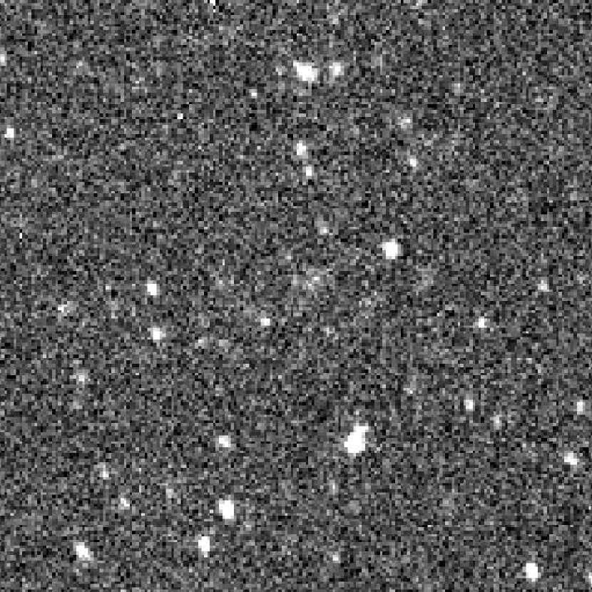
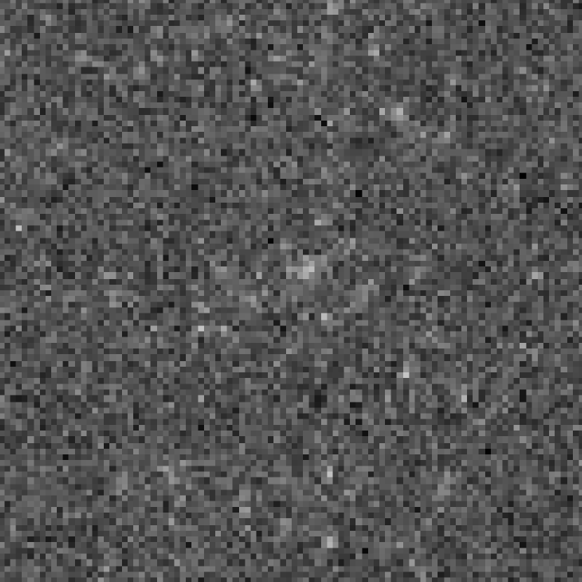
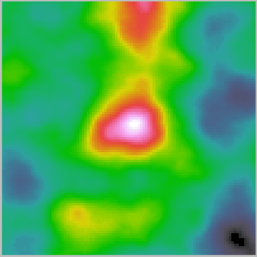
Figure 1: Three panel image illustrating the reduction process for a $140\arcmin\times 140\arcmin$ region, centered on a cluster with a spectroscopic redshift $z$=0.80. The left panel is the bias-subtracted, flatfielded drift-scan data. The middle panel shows an intermediate stage in the reduction process in which detected objects have been replaced with locally drawn, random sky pixels. This image is then convolved with an exponential smoothing kernel of scale length 10$\arcsec$, resulting in the image shown in the panel on the right. Sextractor is utilized to detect positive fluctuations in the smoothed data.

4.1 Bias Subtraction and Flatfielding

Bias subtraction is performed for the drift-scan data using overscan regions in both dimensions. The overscan region perpendicular to the readout direction is 30 pixels wide; the overscan region parallel to the direction of readout is 98 pixels wide for half of the scans, and 10 pixels wide for the rest. To model the bias, we average across the width of the overscan region, and then apply a symmetric Savitsky-Golay smoothing filter (60 pixels in width) along the length of the overscan region to reduce pixel-to-pixel noise (Press et al., 1992). Rms variations in the subtracted bias are $\sim$0.1%. High precision in this step is important, as residual variations can induce spurious detections. Fortunately, removal of the bias is augmented by subsequent reduction stages. For example, some of the residual variation along the readout direction will be removed during sky subtraction, and in both directions residual variation is damped by $\sqrt{2}$ when the images are combined.

Accurate flatfielding of the data is also critical. The reduced data must have residual flatness variation of less than 0.2% ($\mu_{W}\sim$ 28.3 mag arcsec^-2), or else these variations will be the dominant source of noise limiting cluster detection. A key property of drift-scan data is its intrinsic uniformity. With drift scans, pixel-to-pixel variation is minimized because data are clocked across the chip, so sensitivity variations are a concern only perpendicular to the readout direction (at a level $\sim$ 2% in our raw data). Consequently only a one-dimensional flatfield is required, for which the Poisson noise can be reduced significantly relative to a two-dimensional flatfield by averaging along the direction of readout. To reduce the flatness variation to the desired level, we apply two stages of flatfielding. In both stages we use a set of 4 or 5 scans to construct a sigma-clipped, median averaged flatfield. (For a given right ascension, typically four of the scans are taken consecutively one night, and the other five are taken consecutively on a different night.) Each scan is 20,000 pixels in length and the typical sky level in $W$ is $\sim$100 counts, so the associated Poisson noise is 0.035% per column. The first stage of flatfielding immediately follows bias subtraction and reduces sensitivity variation from 2% to 0.4%. Subsequent to this stage, we use the IRAF routine fixpix to interpolate across the three bad columns in our drift scans (see Figure 4.2). The second flatfielding stage is designed to remove the 0.4% residual variation. To eliminate contamination from resolved objects, which may lead to correlated variations across columns, this second stage is run after all detected objects have been replaced with local sky pixels (see §4.2), and after temporal fluctuations in the sky level have been subtracted along the direction of readout (see §4.3). Figure 4.2 shows a typical pair of flatfields resulting from these two stages of flatfielding. Subsequent to this final flatfielding all scans are flat to $\lesssim$0.2%, with an rms residual variation of $\sim$0.1%.

4.2 Object Removal and Masking

Next, we remove all stars and galaxies that are individually detectable in the images using a modified version of the Faint Object Classification and Analysis System (FOCAS) (Jarvis & Tyson 1981; Valdes 1993; modifications described in Dalcanton et al. 1997). The basic strategy is to use FOCAS to detect all objects in the scans and then clean out objects down to a limiting aperture magnitude. Using an aperture of radius 5 pixels, we choose a limiting aperture magnitude m_W=22.8, which roughly corresponds to a 4-$\sigma$ detection in an individual scan.

Typical flatfields generated in reducing the scans. The upper panel shows the 1-D flatfield applied to the raw data, which corrects initial variations of order 2%. The sharp vertical features in this panel correspond to bad columns. The lower panel shows the second pass flatfield which is applied to scans after sky subtraction and cleaning. Subsequent to this stage, residual variations are at the level of 0.1%.

One inherent obstacle in using FOCAS for detection is that drift scans have a time-variable component to the sky level. This variability in turn means that the rms of the sky will vary through the image. Because FOCAS uses a fixed sigma threshold throughout the scan, the sky variation results in variable depth for the FOCAS catalog. The solution we employ is to calculate and input to FOCAS the sigma corresponding to the lowest sky level in the scan. The catalog then goes too deep in some locations, but is deep enough everywhere to uniformly implement the desired aperture magnitude limit for cleaning, and yields uniform object removal throughout the image. The actual cleaning is accomplished with a modified version of the FOCAS routine CLEAN, which replaces object (a) Mask size as a function of FOCAS isophotal magnitude and isophotal area. Points indicate a representative subset of objects detected in the survey, with the lower branch containing stars and the upper branch containing galaxies. Solid lines demarcate changes in mask size, with no masking applied to objects in the lower right region of the plot. For stars, isophotal magnitude is the primary factor driving the mask size; for galaxies, isophotal area is the more important factor. An inflection occurs in the stellar branch at m$\sim$15 and corresponds to the magnitude above which stars are saturated in this data set. (b) Stellar mask size as a function of isophotal magnitude. (c) Galaxy mask size as a function of isophotal area.

pixels with local sky pixels. When cleaning, the replacement region corresponds to the isophotal area of the detection, plus a growth region, the width of which is a function of the 5$\arcsec$ aperture magnitude of the object. For objects with $m_{ap}<16.8$, the width of the growth region is 8 pixels; for objects just above the cleaning threshold the width of the growth region is 2 pixels. There are two notable cases in which this cleaning proves insufficient, however. Saturated stars and large galaxies both leave residual flux in Sky fits for a set of nine scans at the same right ascension. The mean level of a given fit is arbitrary as these have been renormalized and plotted in order of decreasing declination, with a mean offset of 2.5 counts between each scan. This figure illustrates the amplitude of the sky fluctuations, and also the need for a discontinuous component to the sky level in some cases.

the image beyond the cleaning radius, and consequently are masked.

To mask, we identify the objects for which cleaning is insufficient. Figure 4.2$a$, which shows isophotal area as a function of isophotal magnitude, illustrates how we perform this identification. Objects on the upper branch in this figure are galaxies; those on the lower branch are stars. For large galaxies, we use the isophotal area to determine the size of the mask. For the saturated stars (m${}_{W}\lesssim$15), we instead use the isophotal magnitude. The radii of the circular masks as a function of isophotal area and magnitude are shown in Figures 4.2$b$ and 4.2$c$. For both stars and galaxies we take a conservative approach and apply large masks, with the typical mask radius for galaxies being $\sim 5$ times the isophotal radius. In addition to bright stars and galaxies, scan edges and linear features in the data such as bleed trails are also masked. The net effect of all masking is a 28% reduction in the total area of the survey.

4.3 Sky subtraction

After the images have been masked, a large gradient in the sky level persists along the direction of readout of the scans ($\alpha$). The gradient is the result of temporal variation in the sky brightness during the observations. This component of the sky is generally smoothly varying; however, sharp changes in the sky level do exist. These sharp changes can be due to bleed trails, scattered light from bright stars in the field of view, or internal reflections in the optics. Both the smooth and sharp components can result in sky brightness fluctuations of $\Delta\mu\sim$0.3 mag arcsec^-1. In the absence of sharp edges, an effective way of removing the sky is to average the columns in a scan and then apply Savitsky-Golay filtering. This approach minimizes random small-scale noise while preserving the slowly varying component of the sky that we are trying to model. Unfortunately, if there are any sharp changes in the sky level the Savitsky-Golay filtering also induces large errors in the modelled sky level near the edges. To circumvent this problem, a very simple edge detection algorithm is employed prior to Savitsky-Golay filtering. Once edges have been detected and the magnitude of the change has been determined, a step function representation of this component of the sky level is constructed. This discontinuous component is subtracted from the image, leaving only the smoothly varying component of the sky, which can then be modelled with the approach described above. Figure 4.2 shows sky fits for a set of scans at the same right ascension, illustrating the procedure described above. The presence of a discontinuous change in sky level can be seen in the fourth fit from the top. As a precaution, we also mask all data within 20 pixels of detected discontinuities. Subsequent to this fitting procedure, all images are normalized to have the same median sky level.

Temporal effects are not the only source of large scale variation in the sky level. In addition, two-dimensional structure is expected to be present due to galactic cirrus, reflection nebulae, scattered light, and saturated bright stars. To correct for these large scale variations we employ boxcar smoothing. Each scan is smoothed on a scale of 140$\arcsec$, and then the smooth, large-scale component of the sky is subtracted. This scale is sufficiently large that high redshift clusters have a negligible contribution to the smoothing.

4.4 Registration

An important step in this survey is registration of the scans. Registration is required for several reasons, each of which requires a different degree of accuracy. First, the cleaned images must be aligned with an accuracy greater than the scale of the smoothing kernel, or else cluster fluctuations will be diluted by the misalignment. For our smoothing scale of 10$\arcsec$, the scans must be aligned to $<$3$\arcsec$. Second, we use the registration to generate $\alpha,\delta$ coordinates for cluster candidates, which are used for follow-up observations. For this purpose, accuracy of a few arcseconds is generally acceptable. Finally, mosaics are constructed from the images prior to object removal. these mosaics should be aligned well enough that their profiles are not bimodal although the cluster identification criteria are fairly robust to misalignment. Typical seeing during observations was between 1 and 1.5$\arcsec$, so the alignment should be good to $<$1$\arcsec$. Considering that each scan is 3.8^∘ (20,000 pixels) long and that the curvature of a scan varies with declination, subarcsecond accuracy is a challenging requirement.

To register the images, the IRAF routine DAOFIND is used to locate all bright stars in a scan. Using an initial estimate for the scan center and curvature of the scan (see Appendix A for a discussion of projection effects for Great Circle scans and regular scans), these stars are cross-correlated with the HST Guide Star Catalog. Actual values for the scan center and the curvature are determined by maximizing the correlation with the guide stars. This cross-correlation is done for each scan, so that the scans are directly tied to a global coordinate system, which prevents the accumulation of error inherent in using relative offsets. The resulting alignment accuracy between scans is acceptable. Near the centers of scans, the alignment is generally good to $<$0$\,\farcs$5. This quality degrades towards the ends as small errors in curvature are amplified. In the worst regions a maximum error of 1$\farcs$5 is reached; however, generally the error at the ends of scans is $\sim$ 1$\arcsec$.

4.5 Mosaicing

The code we use to mosaic the scans is a modified version of the DIMSUM package for IRAF. Two mosaics are constructed at each right ascension - one of the scans prior to object removal and one after object removal. Our only noteworthy modification to the DIMSUM package is with regard to the way in which masking is handled. Masking was used for:

1. Bright stars and galaxies, for which cleaning is insufficient.

2. Bleed trails and sharp changes in the sky level, near which the sky fit may be poor.

3. Image edges, where FOCAS may fail to detect some objects.

When mosaicing, masking can be handled in two ways: one can either require that a region be unmasked in both overlapping scans for it to remain unmasked, or one can require that it be unmasked in only one of the scans and use the pixel values from the unmasked scan. The first option is preferrable for objects intrinsic to the image (e.g. bright stars), and also has the advantage of maintaining uniform survey depth. However, the second option is useful if the region being masked is small or narrow, in which case continuity may be more important than uniform survey depth (particularly for FOCAS object detection). We utilize the first approach for bright objects, bleed trails, and sharp changes in sky level, but use the second approach for scan edges.

4.6 Smoothing and Detection

We next convolve the cleaned images with a smoothing kernel to increase signal-to-noise prior to cluster detection. Optimal signal-to-noise is achieved when both the kernel profile and scale are matched to cluster properties (see Phillipps & Davies, 1991, for a thorough discussion of the topic). For an exact match, the surface brightness value in the convolved image will correspond to the central surface brightness of the object, while mismatch will lower the observed central surface brightness. We expect some degree of mismatch in this survey both because we are probing a range in redshift and cluster mass (and hence scale), and also because it is doubtful that high-redshift clusters Fractional decrease in the observed surface brightness as a function of the relative mismatch between the filter scale length, $\alpha$, and the optimal scale length, $\alpha_{optimal}$. The curves shown correspond to an exponential filter convolved with exponential, Hubble, and de Vaucouleurs profiles.

exhibit symmetric, uniform surface brightness profiles. Further, we choose to employ an exponential kernel for the LCDCS - which is probably not the correct profile for high-redshift clusters. Consequently, it is useful to assess the impact of these factors upon our sample.

To quantify the expected degradation due to our choice of kernel, we compute the maximum cross-correlation for convolution of an exponential kernel with Hubble and de Vaucouleurs profiles. If the scale of the kernel is optimally matched to the scale of the profile (see below), then use of an exponential kernel results in net decreases in the observed peak surface brightness of 4% and 9%, respectively, for these profiles. Thus, we expect that our use of an exponential kernel has minimal impact upon our detection efficiency. Of greater importance is the choice of scale length for the kernel. Figure 4.6 shows the fractional decrease in the observed surface brightness for various profiles as a function of the ratio of the actual kernel scale length to the optimal kernel scale length. For all profiles, the fractional loss is $<$15% when the scale is matched to within a factor of two.

For the LCDCS, we set the scale length of our kernel to optimize our ability to detect clusters at $z=1$. If we assume a Hubble profile for the cluster, then optimal scale length for our kernel is $\alpha=0.6r_{c}$, where $r_{c}$ is the Hubble core radius. (This is equivalent to setting the scale length such that both the exponential and the Hubble profile fall off to half the central surface brightness at the same radius). For rich clusters typical core radii are Radial filter weights from the LCDCS, PDCS (Postman et al., 1996), and an optical survey by Lidman & Peterson (1996). The filter weight is defined as $rf(r)/\int rf(r)dr$, where $f(r)$ is the filter profile. For the LCDCS most detection power is contained within 300 kpc at $z$=0.7. In contrast, the other surveys shown, which use galaxy counts, have most of their detection power at much larger radii.

$r_{c}\sim 100-150h^{-1}$ kpc, so the kernel size should be 60-90 $h^{-1}$ kpc (12-18$\arcsec$ at $z=1$ for an $\Omega_{0}=0.3$ open model, or 11-16$\arcsec$ for an $\Omega_{0}=0.3$ flat model). Since the core radii for clusters at this redshift may be smaller than local systems, we choose to use a slightly smaller scale length of 10$\arcsec$. This choice of smoothing kernel does yield a factor of three mismatch at $z=0.4$, which corresponds to about a 20% fractional loss for Hubble or de Vaucouleurs profiles.

The extent of the kernel used for this survey is significantly smaller than those utilized for other optical surveys, with all the power coming from within 250 $h^{-1}$ kpc (see Figure 4.6). Because other surveys rely on number counts, by necessity their kernels typically have scale lengths of order 1 Mpc in order to include enough galaxies to generate a statistically reliable signal. Unfortunately, use of such a large kernel increases the likelihood of inclusion of poor systems due to projection effects or large scale structure. Our small kernel minimizes projection effects and, because our method can detect cluster cores in the absence of a well-formed envelope, we have a greater probability of detecting clusters at early evolutionary stages. Conversely, it is possible that this technique will produce multiple, distinct detections for clusters with significant substructure. While this effect is a concern, we anticipate that it is a minor issue because we see no enhancement in the angular correlation function at small separations. Another possibile concern is whether we detect subclumps of dwarf galaxies in nearby Abell clusters. Again, we see no evidence of correlation between the locations of our candidates and Abell clusters in the survey region (see Figure 7.1 in §6), and therefore expect that such detections do not significantly impact the catalog.

Once a smoothed version of a scan region has been generated, SExtractor v2.1.6 (Bertin & Arnouts, 1996) is employed to detect positive brightness fluctuations. SExtractor is used instead of FOCAS because of its computational efficiency and a superior ability to deblend overlapping detections. The detection threshold is set such that all fluctuations with peak surface brightness in excess of $\mu_{W}$=28 mag arcsec^-2 ($\sim 5.4\times 10^{-3}$ counts s^-1 arcsec^-2) are identified. For a typical scan set covering 7.6 square degrees this procedure yields $\sim$2500 detections. Of these, roughly 65% are in the 5.9 square degree overlap region used for the cluster survey (of which $\sim$30% is typically masked). About 5% of these detections are galaxy clusters at $z$$>$0.3; the rest are contamination. We use an automated classification technique, described in the next section, to identify viable cluster candidates.

5 Cluster Identification

A critical element in creating the cluster catalog is identification of viable cluster candidates and rejection of other sources of surface brightness fluctuations. Several techniques were explored for isolating cluster candidates including hierarchical, divisive, and fuzzy clustering algorithms (Gordon, 1981; Jain & Dubes, 1988) and automated Bayesian classification (Cheeseman et al., 1988; Goebel et al., 1989), with each method using as input a generalized set of statistics characterizing the detection image. A drawback of these algorithms though is that the physical meaning of the resulting classes is not always clear, nor is it straightforward to reproduce these classes for simulated data or new samples (particularly for the fuzzy and Bayesian techniques). Consequently, we instead choose a more intuitive and easily reproducible approach for extracting cluster candidates that yields a success rate comparable to the other approaches. We identify classes of objects that induce fluctuations and separately isolate these classes utilizing specific properties unique to the given type of object.

To do so, we employ information from both the smoothed and original images. From the smoothed maps, we use:

1. The observed peak brightness, $\Sigma_{obs}$, of the detected surface brightness fluctuation. It is defined as the maximum surface brightness value in any pixel in the fluctuation, and the units of $\Sigma_{obs}$ are counts s^-1 arcsec^-2.

2. The concentration, $C$, of the observed surface brightness fluctuation. We define the concentration in terms of the fraction of pixels above a given threshold for two regions - an inner, circular region of radius 15$\arcsec$ and an outer annulus extending from 15-30$\arcsec$. $C$ is one minus the ratio of the fraction above the threshold in the outer annulus, $f_{o}$, to the fraction above the threshold in the inner region, $f_{i}$:

   $$C\equiv 1-\frac{f_{o}}{f_{i}}.$$ (1)

   The threshold is set such that $\Sigma_{threshold}$=4.2$\times 10^{-3}$ counts s^-1 arcsec^-2= 2/3 $\Sigma_{lim}$, the limiting surface brightness of the final catalog (see §6).

3. The fraction of the detection region that is masked. We measure the fraction of masked pixels within a $1\arcmin\times 1\arcmin$ square region centered on the surface brightness fluctuation.

From the original images we obtain photometric data about objects located near the fluctuation, which enables us to discern whether the detection was caused by a low surface brightness galaxy, bright star, or nearby galaxy rather than by a cluster. Specifically, we measure:

1. The 5$\arcsec$ aperture magnitude, $m_{ap}$, of the brightest object (lowest m_ap) located within 15$\arcsec$ of the peak of the surface brightness fluctuation detected in the smoothed data.

2. The aperture magnitude, total magnitude, central surface brightness, and full-width half maximum of the non-stellar object with the brightest $m_{ap}$ located near the detected fluctuation. In identifying this object we consider all sources located within 15$\arcsec$ of either the peak or the centroid of the detected fluctuation. An object is designated non-stellar if the stellarity index $S<$0.97 or $m_{ap}$$>$20. The latter constraint reflects a preference at fainter magnitudes to be conservative and potentially include a few stars rather than reject galaxies as stars. As will be described in §7, this aperture magnitude is used to estimate cluster redshifts, and it is preferrable to occasionally underestimate a redshift due to stellar contamination rather than overestimating the redshift due to identification of the brightest cluster galaxy as a star. The total magnitude, $m_{T}$, is mag_best in SExtractor.

3. The aperture magnitude, total magnitude, central surface brightness and full-width half maximum of the object with the lowest $m_{T}$ located withing 15$\arcsec$ of either the peak or the centroid of the detected fluctuation.

4. The number of galaxies, $n_{gal}$, brighter than $m_{ap}$=22 mag within 30$\arcsec$ of the fluctuation.

The quantities listed above prove sufficient for classification of most detected surface brightness fluctuations. Prior to classification, we eliminate all detections that lie in regions where E($B$-$V$)$>$0.10 (Schlegel, Finkbeiner, & Davis, 1998). This criteria removes all detections at $\alpha$$>$15h12m, where the data are at low galactic latitude, and an additional 32 detections at lower right ascension that would otherwise be included in the statistical catalog (see §6). We also eliminate all detections lying in regions that, based on visual inspections of IRAS maps obtained from SkyView (McGlynn, Scollick, & White, 1996) and the smoothed optical maps generated in this work, contain galactic cirrus with significant structure. We do so because galactic cirrus both reflects optical light and produces extended red emission from 6000-8000Å(Guhathakurta & Tyson, 1989; Szomoru & Guhathakurta, 1998), and nonuniformity in this emission/scattered light generates surface brightness fluctuations that are indistinguishable from cluster-induced fluctuations. An example of this phenomenon is shown in Figure 5. Finally, to preserve a constant threshold for the survey, a target is only considered a cluster candidate if the detection lies in a region that was observed twice during the course of the survey. All other detections are flagged and removed from further consideration. We then proceed by identifying the physical origins of the remaining fluctuations and sequentially isolating classes of objects. The types of objects, and parameters used to isolate them, are described below.

Stars - As described in $\S$ 4, all detected objects in the drift-scan data are replaced with local, random sky pixels. This procedure effectively removes most resolved objects; however, for bright stars the ‘sky’ pixels used to replace the star often contain a non-negligible amount of light from the wings of the stellar point spread function. As a result, a surface brightness fluctuation is produced coincident with the star for stars with 14.5$<$m_ap$<$18.5. For m_ap$<$14.5 the stars are masked; for m_ap$\gtrsim$18.5 the stars are sufficiently faint that they do not induce detectable fluctuations. Fluctuations induced by bright stars are cleanly isolated using the stellarity index and magnitude of the brightest object near the fluctuation. We classify a detection as being induced or strongly influenced by a star if the brightest object within 15$\arcsec$ of the peak of the detection has a stellarity index $S$$>$0.9 and $m_{ap}$$<$18.5. Stars are responsible for half of all detections.

Galaxies - Individual galaxies can also cause detectable surface brightness fluctuations if they have significant flux at large radii. As with bright stars, the local ‘sky’ pixels used to replace the core of the galaxy produce a surface brightness feature coincident with the original location of the galaxy. To minimize contamination of the cluster catalog by these detections, we impose two criteria. First, we classify a detection as a galaxy-induced if there is a galaxy with $m_{T}$$<$18.75 within 15$\arcsec$ of the peak or centroid of the detection (which is about a quarter of a magnitude brighter than a typical BCG at $z$=0.30).

We augment this procedure with a second cut that takes into account the surface brightness of the detection and the number of galaxies within 30$\arcsec$ of the detection. If the brightest galaxy near the fluctuation is the brightest cluster galaxy (BCG), then the fluctuation should be significantly brighter than one induced by an isolated, local galaxy of the same apparent magnitude. In addition, at $z$$\sim$0.3 we should be able to identify projected galaxy overdensities associated with real clusters. To discriminate low-redshift clusters from isolated galaxies, we define the parameter $p_{gal}$ such that

$$p_{gal}=\sqrt{(2.5*(\Sigma_{obs}/\Sigma_{det}-1))^{2}+(n_{gal}-1)^{2}},$$ (2)

where $\Sigma_{det}$=5.4$\times 10^{-3}$ counts s^-1 arcsec^-2is the detection threshold of the survey. Using this parameter, we classify detected fluctuations as galaxies if

$$p_{gal}<2.5-6(m_{ap}-20).$$ (3)

This criteria is empirical, constructed from visual inspection and follow-up imaging of candidates at 10h$<$$\alpha$$<$10h15m ($\sim$5% of the survey). No detections are eliminated when $m_{ap}$$\gtrsim$20.4, which means that this cut has Comparison of an IRAS 60$\mu$ image (left) and smoothed optical map (right) of a small section of the survey. The images are 1.9$\arcdeg\times$3.9$\arcdeg$ in size. East is up and north is to the right. Note the large cirrus spike evident in the center of the IRAS image. In the optical image the large scale structure of the spike is filtered during sky removal; however, small scale features persist and can be seen in the optical map. Consequently, via inspection of the IRAS and optical maps we catalog these regions and reject all detections in these areas. Note also the satellite trail at the lower edge of the optical image. Satellite detections that survive the automated selection criteria discussed in §5 are manually removed from the final sample.

no impact on the final catalog at $z_{est}\gtrsim$0.35 (see §7.3). Together the galaxy identification criteria eliminate 14% of all detections.

Low Surface Brightness and Dwarf Galaxies - After elimination of fluctuations caused by stars and galaxies, we identify detections induced by low surface brightness galaxies (LSBs) and dwarf galaxies. To identify these galaxies, we rely on the SExtractor information from the original images for the two galaxies within 15$\arcsec$ that have the brightest aperture and total magnitudes. Qualitatively, if a galaxy is a nearby LSB or dwarf, we expect that the central surface brightness will by definition be low, the FWHM will be relatively large since the galaxy is nearby, and the total magnitude will be much larger than the aperture magnitude (due to the previous two traits). We employ a two-stage approach to eliminating LSBs. First, we identify detections as potentially induced by LSBs if $m_{ap}$-$m_{T}$$>$1.25 for either of these two nearby, brightest galaxies. Second, we define the parameter, $p_{LSB}$,

$$p_{LSB}=FWHM-1.2m_{T}+11.5,$$ (4)

and eliminate detections as likely LSBs if $\mu_{0}$$>$22 mag arcsec^-1 and $p_{LSB}$$>$0 for either of these two galaxies (see Figure 5). This constraint, which is again empirical, is calibrated via visual inspection. A total of $\sim$250 detections in the entire survey are classified as LSB candidates based upon these criteria. By visual inspection of these detections, we estimate that $\sim$5 clusters with $\Sigma_{obs}$$>$$6.25\times 10^{-3}$ counts s^-1 arcsec^-2are lost due to misidentification as LSBs. Conversely, $\sim$ 20 LSBs are mistakenly identified Criteria used to isolate LSBs. Filled circles are clusters, triangles are low surface brightness galaxies, and circled crosses are systems that are visually ambiguous when classified by eye from the scans. Detections with $p_{LSB}$$>$0 are identified as probable LSBs. The data plotted represent data from the entire survey. Only the first 10% of the survey region was used to calibrate this division, but all sources designated as LSBs or clusters were visually inspected after automated classification to verify the effectiveness of this procedure.

as clusters and included in the final catalog.

Partially masked detections - We next eliminate from the statistical sample all other detections for which greater than 10% of the detection region is masked. Such obscuration of the detection region leads to difficulty in determining the true cause of a detection, and consequently results in increased contamination of the cluster sample.

Scattered light and assorted spurious reduction-induced signals - Subsequent to the removal of all of the sources listed above, $\sim$8% of the total detections remain. Of these, the principal remaining contaminants are sources arising from scattered light and signals related to the reduction process. As a class, these detections are characterized by low peak surface brightness and large spatial extent relative to the clusters. To isolate these, we use the concentration measure, $C$, as a discriminant. Detections of this type are on average less concentrated (lower $C$) than clusters of comparable surface brightness. The division between the two classes is shown in Figure 5.

Satellites and Bleed Trails - Satellites and bleed trails from saturated stars, because they are not detected by FOCAS and replaced with sky pixels, also induce fluctuations. These sources are rare and easily identifiable, and so they are identified by visual inspection. This is the only aspect of the classification procedure that is not automated.

Tidal Features - Another source of detections is tidal features in nearby, interacting systems. We do detect fluctuations induced by large tidal features; however, we do not identify these as a distinct class of objects when generating the cluster catalog. Tidal features, because of their varied morphologies, are difficulty to identify via Criteria used to eliminate spurious detections. Filled circles are clusters, triangles are spurious detections, and circled crosses are systems that are visually ambiguous. The data plotted are drawn from the entire survey region.

automated criteria. Fortunately, however, the surface density of interacting systems capable of inducing detections is low. From visual inspection, we estimate the fractional contamination by tidal tails is $\sim$1% in the final catalog.

Chance Galaxy Superpositions - Chance superpositions of several field galaxies with magnitudes near the survey limit provide a final source of contamination. Such detections are indistinguishable from true cluster detections, and so can only be eliminated with deeper follow-up imaging. While it is difficult to robustly estimate the magnitude of this contamination directly from the survey data, these superpositions may be the primary source of false detections in the final catalog (see 7.2 for observational constraints on the net contamination rate).

Clusters - All of the remaining 2670 detections are cluster candidates. As will be discussed in §6, not all of these systems are included in the final statistical catalog; however, we consider all these detections to be viable candidates. The properties of the sample are discussed in further detail in §7.

6 The Catalog

Having established our selection criteria, we now define the main, statistical catalog for the Las Campanas Distant Cluster Survey. This statistical sample is designed to be an automated, reproducible catalog with which to study properties of the cluster population as a whole. For this catalog, we impose two additional constraints beyond those discussed in §5. First, we restrict the catalog to detections with $\Sigma_{obs}$$>$$6.25\times 10^{-3}$ counts s^-1 arcsec^-2. This restriction is due to relatively high contamination for fainter systems, as determined by follow-up imaging. Second, we restrict the sample to clusters at $z$$>$0.30. Below this redshift incompleteness and confusion with individual galaxies become significant issues.

Redshift distribution of clusters in the statistical catalog.

There are a total of 1073 cluster candidates in the statistical catalog. These candidates are drawn from a net survey area, after masking, removal of regions of high extinction, and rejection of data in close proximity to bright stars and galaxies, of 69 square degrees. Equivalently, the projected density of cluster candidates is 15.5 per square degree, which is comparable to the PDCS and EIS catalogs (13.4 per square degree for the primary PDCS sample, and 21.1 per square degree for the full EIS sample). As the redshift baselines of these three surveys is slightly different, a more fair comparison is the projected density of clusters at $0.3\leq$$z$$\leq$ 0.8. Within this range, the LCDCS, PDCS and EIS find projected densities of 14.2, 10.8, and 10.7 candidates per square degree, respectively. The higher projected density of the LCDCS is likely an indication that we probe to slightly lower mass, but may also be partly due to higher contamination (see §7.2).

Table 1 lists all candidates in the catalog. For each candidate, we provide an identification number in Column 1, right ascension in Column 2, and declination in Column 3. Estimated redshift, the derivation of which is described in §7.3, is given in Column 4. Subsequent columns list observed surface brightness, $\Sigma_{obs}$, in 10^-3 counts s^-1 arcsec^-2 (Column 5), extinction corrected surface brightness, $\Sigma_{cor}$, in 10^-3 counts s^-1 arcsec^-2 (Column 6), and the $\bv$ extinction from Schlegel, Finkbeiner, & Davis (1998) (Column 8). For the extinction correction, we take $A_{W}$=3 $E$($\bv$), which is the average of the published values for $A_{V}$ and $A_{R}$ (see Figure 2 for a comparison of $W$ with these passbands). Finally, Column 9 contains additional information for some candidates, including notes for objects that from inspection are obviously not clusters. All observed surface brightnesses have an associated uncertainty of 1.6$\times$10^-3 counts s^-1 arcsec^-2(see §7.1); derivation of the uncertainty for the extinction-corrected values is straightforward. Figure 6 gives the redshift distribution of these candidates, and Figure 7.1 shows the projected distribution overlaid with the locations of Abell clusters. In Figure 2 we show detection images for seven candidates covering the redshift range of the survey.

The statistical catalog is the primary sample presented in this paper. However, because the interests of researchers who use this catalog may be diverse, we have also constructed a smaller, supplemental catalog that contains additional cluster candidates. These supplemental targets are detections that failed one or more of the automated criteria for inclusion in the statistical sample, but visually appear to be highly probable cluster candidates. For this supplemental catalog, we maintain the restriction $\Sigma_{obs}$$>$6.25$\times 10^{-3}$ counts s^-1 arcsec^-2, and no attempt was made to recover clusters that were mis-classified as stars, or detection for which more than 50% of the detection region was masked. We do, however, re-evaluate all detections rejected on the basis of extinction, lesser masking, identification as an LSB, or identification as a spurious feature. We also relax the galaxy rejection criteria such that clusters may have $z$$<$0.30 and $m_{T}$$<$18.75. From this extended sample we visually identify 112 additional cluster candidates. Table 2 lists the supplemental targets, including the reason for rejection from the statistical sample. We note that the $\Sigma_{obs}$ values of clusters rejected due to masking should be used with caution, as partial masking can skew this quantity. The redshift distribution of the supplemental catalog is comparable to the statistical catalog for $z$$\lesssim$0.65. At higher redshift there are more candidates in the statistical catalog, due both to contamination in the statistical catalog and failure to visually identify high redshift candidates for the supplemental catalog.

7 Sample Properties

To maximize the utility of this sample, we must constrain four key properties of the catalog. Specifically, we need to determine the completeness of the sample, the contamination rate, the redshift distribution, and the mass limit of the survey as a function of redshift. Further, if possible, we wish to estimate redshifts and masses for individual systems directly from the survey data. We address each of these issues below.

7.1 Completeness

To quantify the completeness of the sample and uncertainties in measured parameters, we run simulations in which a dozen of the detected cluster candidates - including several below the surface brightness threshold of the statistical catalog - are randomly reinserted into the survey data. Information about these clusters, which were selected to span a range of surface brightness and redshift, is given in Table 3. These simulations are specifically aimed at measuring completeness as a function of surface brightness and scatter in the observed values of $\Sigma_{obs}$ for clusters similar to the ones that we detect in the LCDCS. A corollary concern is whether we systematically miss any subset of the cluster population. If so, then the completness rate derived from these simulations will overestimate the actual value. Figure 4.6 implies that our ability to detect clusters is not strongly dependent upon the core radius. In addition, we have obtained survey quality drift-scan imaging of 17 clusters at $z=0.35-0.85$ drawn from published optical and X-ray catalogs to test for any The projected distribution of cluster candidates in the LCDCS, subdivided by right ascension. In all panels, the dashed lines correspond to the declination range of the survey ($-13\arcdeg<\delta<-11.5\arcdeg$). The overlaid circles correspond to the Abell radii for Abell clusters within the field of view of the survey.

systematic bias in our detection method. For this sample, which spans a wide mass range (see Figure 3 in §7.4), our observations have resulted in successful detection on 16/17 clusters (Gonzalez, 2000). The undetected cluster, PDCS 8, has a published 3-$\sigma$ upper limit on the X-ray luminosity, $L_{X}=9.8\times 10^{43}h_{50}^{-2}$ erg s^-1 (0.4-2 keV, $\Omega_{0}=1$) for an estimated redshift $z$=0.6 (Holden et al., 1997). We thus anticipate that we are not systematically missing a significant fraction of the cluster population due to our detection method, but caution that such a bias may exist.

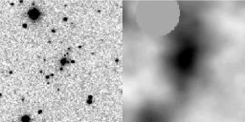
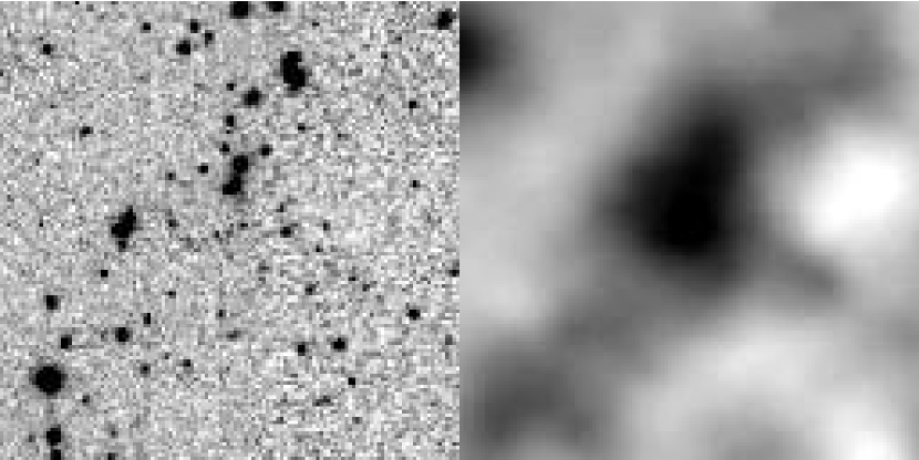
LCDCS 0347 ($z_{est}$=0.30)                                                             LCDCS 0169 ($z_{est}$=0.39)

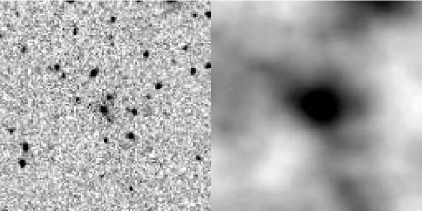
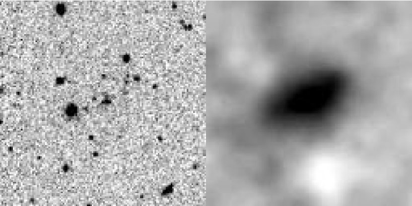
LCDCS 0589 ($z_{est}$=0.50)                                                             LCDCS 0795 ($z_{est}$=0.59)

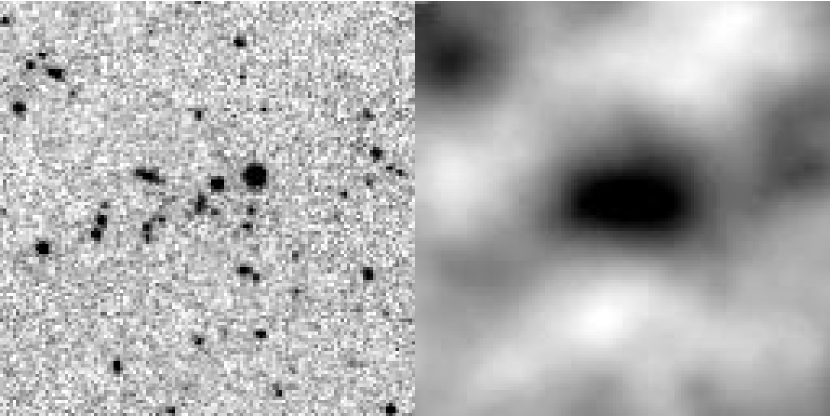
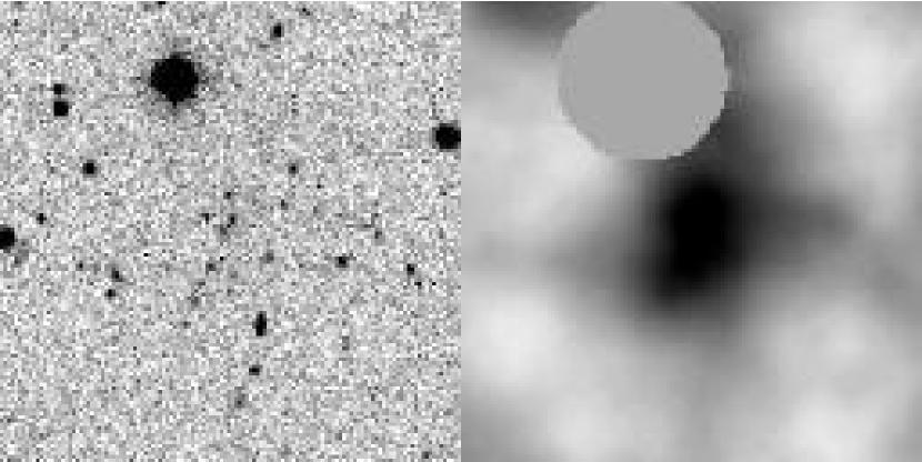
LCDCS 0827 ($z_{est}$=0.71)                                                             LCDCS 0130 ($z_{est}$=0.80)

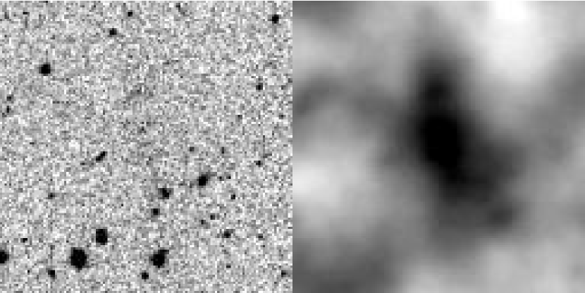
LCDCS 0797 ($z_{est}$$>$0.85)

Figure 2: Detection images for seven of the candidates in the LCDCS catalog. The candidates shown were chosen to uniformly span the redshift range of the survey. Further, all candidates shown have $\Sigma_{obs}$=9-9.5$\times$10^-3 cts s^-1 arcsec^-2, except for LCDCS 0797 ($\Sigma_{obs}$=7.9$\times$10^-3 cts s^-1 arcsec^-2).

To quantify the completeness and scatter, we insert the clusters throughout the entire survey region. The inserted data consist of 140$\arcsec\times$140$\arcsec$ (200$\times$200 pixel) image sections centered on the clusters. Insertion points are chosen at random, but with the criteria that the position be in the overlap region of the survey and not lie beneath a mask. No pre-selection is made based upon extinction or proximity to prominent cirrus features, and so 16% of the inserted clusters are rejected on these grounds. These rejected clusters are not considered in computing the completeness, as they are already accounted for in the determination of the effective survey area. We use different random locations for each candidate, and each of the 12 candidates is inserted into the survey images 264 times (12 insertions per candidate in each of the 22 mosaics). To avoid crowding effects, only 72 clusters are inserted into a mosaic for each run of the simulations.

We track the detection rate and the rate at which a candidate will be included in the statistical catalog. In addition to determining the completeness, we also use this data to quantify the rms uncertainty in $\Sigma_{obs}$. We find that the standard deviation is $\sigma_{\Sigma}$=1.6$\times 10^{-3}$ counts s^-1 arcsec^-2, independent of $\Sigma_{obs}$, which corresponds to roughly 25% uncertainty at the faint limit of the statistical catalog. This scatter defines the limiting precision with which we Fractional completeness of the catalog as a function of surface brightness. Triangles indicate the probability that a cluster is detected, assuming that it does not lie directly beneath a mask. Circles indicate the probability that a cluster is included in the statistical catalog. The solid curve is an analytic model for the completeness of the statistical catalog (see text).

can estimate velocity dispersions for candidates in the sample (see §7.4).

The results of these simulations can be seen in Figure 7.1 and are listed in Table 3. The detection rate is near 100% for $\Sigma_{obs}$$>$8.5$\times 10^{-3}$ counts s^-1 arcsec^-2. Of these bright candidates, 78% qualify for inclusion in the statistical catalog. The majority of those that fail to be included in the catalog are rejected due to proximity to either a star or a mask, which together eliminate $\sim$20% of candidates. Proximity to bright galaxies eliminates most of the remaining detections. Assuming that the incompleteness at low surface brightness is the result of Gaussian uncertainty in $\Sigma_{obs}$, the expected completeness of the statistical catalog can be modelled as

$$F(\Sigma_{obs})=F_{0}\times\frac{\mathrm{erf}((\Sigma_{obs}-\Sigma_{lim})/\sqrt{2}\sigma_{\Sigma})+\mathrm{erf}(\Sigma_{obs}/\sqrt{2}\sigma_{\Sigma})}{1+\mathrm{erf}(\Sigma_{obs}/\sqrt{2}\sigma_{\Sigma})},$$ (5)

where $F$ is the fractional completeness, and $F_{0}$ is the maximum fractional completeness at high $\Sigma_{obs}$. This model is overlaid in Figure 7.1 with $\Sigma_{lim}$=6.25$\times 10^{-3}$ counts s^-1 arcsec^-2, $\sigma_{\Sigma}$=1.6$\times 10^{-3}$ counts s^-1 arcsec^-2, and $F_{0}$=0.78.

7.2 Contamination Rate

We utilize follow-up imaging to assess the false detection rate in the LCDCS. While this approach provides the most direct means of quantifying the contamination, care must be taken to insure that the derived result is not biased. The imaging that we have can be divided into two sets, both of which are described in detail in Nelson et al. (2001a). The first set is deep, multi-color imaging obtained in 1996 and 1997 with the Las Campanas 1m and 2.5m telescopes. From these runs, most targets have in excess of 1 hour of imaging on the 1m (or 20 minutes on the 2.5m) in both $V$ and $I$. These data are sufficiently deep to determine whether a candidate is a cluster; however, some of the targets observed were included specifically because they looked promising in the drift-scan imaging. As a result, an assessment of the contamination based upon these data may underestimate the true contamination rate. The second set of data consists of shallower, $I$-band imaging obtained with the same telescopes in 1998. For this run care was taken to avoid inducing a similar selection bias, and the candidate clusters that were observed are representative of the sample as a whole. Because this data set is shallow, some true clusters may be incorrectly identified as spurious, and so an assessment based upon this data may overestimate the true contamination rate.

For each candidate we compute the number density of galaxies within a 100 $h^{-1}$ kpc aperture centered on the surface brightness fluctuation ($\Omega_{0}$=0.3, $\Omega_{\Lambda}$=0.7; see §7.3 for an explanation of the redshift estimates). We classify targets as clusters if the number density of galaxies in this aperture exceeds the background level by 2-$\sigma$. Furthermore, we test the probability that random number density fluctuations in our fields will exceed this threshold by computing the density contrast for a complementary set of random locations. For the deep, multi-color data set we find that 23/32 (72%) candidates and 3/32 (9%) random fields exceed this threshold. We therefore derive a net contamination rate of 31$\pm$9% (i.e $n_{cl}/N=(n-n_{random})/(N-n_{random})$, where $N$ is the total number of targets, $n$ is the number of $>$2-$\sigma$ detections, and $n_{cl}$ and $n_{random}$ are the number of cluster and random field detections). For the shallower data set we find that 42/57 (74%) of candidates and 4/57 (7%) of random fields exceed this threshold, yielding a net contamination rate of 28$\pm$7%. Because we expect that the two data sets provide lower and upper bounds on the contamination rate, the concurrence of these two estimates is encouraging. Combining the data sets, our estimate of the contamination rate is 29$\pm$5%, with the quoted error bar reflecting purely Poisson uncertainty. We also intend to use additional deep, multicolor observations for contiguous subfields, including data from the Deep Lens Survey, to provide an improved constraint in the near future.

Finally, the fractional contamination increases with estimate redshift, which is a consequence of the method we used to estimate redshifts. As described in §7.3, we estimate redshifts for cluster candidates using the BCG magnitude-redshift relation. For false detections (which by definition lack a BCG), the galaxy identified as the “BCG” will be a random field galaxy along the line of sight. As a result, the distribution of redshifts assigned to false detections is determined by the magnitude distribution of field galaxies. A detailed discussion of the redshift dependence of the contamination is provided in Gonzalez (2000).

(a) BCG magnitude-redshift relation with no correction for $\Sigma_{cor}$. The solid line is an unweighted least squares fit to the data of the function given in Equation 8. (b) BCG magnitude-redshift relation including a $\Sigma_{cor}$ correction. The solid line is an unweighted least squares fit to the data of the function given in equation (2). For both plots, only the data points at $z>$0.35 (circles) are used to calibrate the relation. The lower redshift clusters (triangles), which are known clusters that lie in our survey region, lack measured values of $\Sigma_{cor}$. Further, for clusters at $z$$\lesssim$0.1, the photometric aperture is significantly smaller than the BCG, and so is a poor estimate of the total luminosity.

7.3 Redshifts

To calculate an empirical redshift estimate, we obtained LRIS (Oke et al., 1995) spectra at Keck for a subset of 8 LCDCS clusters and 11 clusters from the northern hemisphere pilot survey (Dalcanton, 1995; Zaritsky et al., 1997). These data were used in conjunction with data for 11 additional previously known clusters to calibrate several photometric redshift estimators (see Nelson et al. 2000a). We find that the most efficient means of estimating redshifts directly from the survey data is via the brightest cluster galaxy magnitude-redshift relation. Locally, brightest cluster galaxies have long been known to be good standard candles, with dispersions $\sim$0.3 magnitudes (Humason, Mayall, & Sandage, 1956; Sandage, 1972a, b). Subsequent work by a number of authors has found that the scatter remains remarkably small out to at least z$\sim$1 (Sandage, 1988; Aragon-Salamanca et al, 1993; Aragon-Salamanca, Baugh, & Kauffmann, 1998; Collins & Mann, 1998).

For our calibration data we find comparably small scatter. We identify brightest cluster galaxies in an automated fashion – we search for the brightest galaxy within a 15$\arcsec$ radii of the peak and centroid of the surface brightness fluctuation from which a cluster is detected, and define this galaxy to be the BCG. This automated definition is designed to make the catalog easily reproducible, while minimizing redshift errors due to foreground contamination or failure to identify the BCG within the chosen search radius. Because we are detecting the cores of centrally condensed objects with our technique, there is a high BCG magnitude residuals from Figure 7.2$a$ as a function of $\Sigma_{cor}$, with $\Delta m\equiv m_{observed}-m_{fit}$. Error bars correspond to the photometric uncertainty associated with the observed BCG magnitudes.

probability that the BCG will be coincident with the surface brightness fluctuation. Further, if we do miss the BCG, the second ranked galaxy is typically $\sim$0.5 mag fainter (Nelson et al., 2001b), which corresponds to a redshift error $\delta z\sim 0.1$. Of the 18 clusters used to calibrate this relation (the northern clusters were not used because they were observed in a different filter), in no instance was the galaxy identified as the BCG more than 0.5 mag fainter than predicted by the final, best-fit model.

We find that the magnitude of the brightest cluster galaxy is an effective redshift indicator. Photometry is performed using SExtractor v2.1.6 (Bertin & Arnouts, 1996), and 5$\arcsec$ aperture magnitudes are used. All magnitudes are extinction corrected using the maps of Schlegel, Finkbeiner, & Davis (1998). Figure 7.2$a$ shows the BCG magnitude-redshift relation for our sample, with the line being a best fit to the data of the function:

$$m=M+5\log D_{L}+Bz^{7/4},$$ (6)

where $M$ is the absolute magnitude and $D_{L}$ is the luminosity distance. The last term is an analytic approximation to the $W$-band $E+k$ correction, which is derived using the 1995 Bruzual & Charlot models (Bruzual & Charlot, 1993; Charlot, Worthey, & Bressnan, 1996). For the luminosity distance we fix $\Omega_{0}$=0.3 and $\Omega_{\Lambda}$=0; however, precise choice of cosmology is unimportant due to degeneracy between this term and the evolution term. The scatter in this relation is $\sigma_{m}$=0.36 mag for the calibration data.

To reduce this scatter we test for second-order correlations. Motivated by an observed correlation between $L_{X}$ and $M_{BCG}$ (Hudson & Ebeling, 1997) and our observed correlation between $T_{X}$ and $\Sigma_{cor}$ (see §7.4 and Gonzalez (2000)), we test for a correlation between $\Sigma_{cor}$ and $m_{BCG}$ (Figure 7.3). We find that

$$m_{BCG}\propto-\log\Sigma_{cor}(1+z)^{4}.$$ (7)

To incorporate this correction, which reduces the scatter to $\sigma_{m}$=0.26, we replace $m$ with

$$m_{corrected} \equiv m+A\log\frac{\Sigma_{cor}\ \ \ (1+z)^{4}}{10^{-2}(1+.5)^{4}}.$$ (8)

in Equation 6. Figure 7.2$b$ shows $m_{corrected}$ as a function of redshift. Overlaid is the unweighted least-squares, which yields

$$m_{corrected}=(-21.3\pm 0.15)+5\log D+(1.7\pm 0.4)z^{7/4},$$ (9)

and $A$=1.5$\pm$0.3. This is the equation that we use to estimate redshifts for candidate clusters. For the redshift range of the LCDCS, a magnitude dispersion of 0.26 mag corresponds to a redshift uncertainty of 10-11%. This constitutes a lower limit on the scatter in our redshift estimates, as there are several caveats to our method.

A first concern is that estimated redshifts beyond $z\sim$0.85 are based upon extrapolation beyond the redshift range probed by the calibration sample, and for these clusters the magnitude of the BCG is very near the detection threshold of our survey data. Consequently, in Table 1 we simply list the redshift as $z$$>$0.85 for these clusters. In addition, we caution that the size of the calibration sample is small, and so our estimate of $\sigma_{m}$ is subject to small number statistics.

Finally, we expect that the redshift dispersion for the catalog as a whole is larger than the dispersion for the calibration data due to foreground contamination and occasional miscentering. We assess the robustness of our redshift estimates using the simulations described in 7.1. These simulations reproduce all sources of uncertainty in the estimated redshifts (e.g. foreground contamination, miscentering, scatter in $\Sigma_{obs}$) except for intrinsic BCG magnitude dispersion. Failure to identify the BCG due to miscentering turns out to be a minor issue for the clusters reinserted into the survey data. We find that for these clusters redshifts are underestimated by $\Delta z$$>$0.1 less than 2% of the time, and only 1% of the time will a cluster incorrectly be assigned a redshift $z$$>$0.75. The largest bias in the estimated redshifts is due to foreground contamination. In Figure 7.3, this can be seen as a tail towards low redshift. While negligible at $z$$<$0.5, by $z$=0.8 foreground contamination leads the redshift to be underestimated by $\Delta z$$>$0.1 35% of the time. In addition, dispersion in $\Sigma_{obs}$ induces a Gaussian uncertainty in the estimated redshift of magnitude $\sigma_{z}$=0.02. Combined with the intrinsic dispersion in BCG magnitude, these factors lead us to expect an rms redshift uncertainty of $\sim$13% for low-redshift clusters in the final catalog, rising to $\sim$20% by $z$$\sim$0.8. We Simulated distribution of estimated redshifts for the nine clusters with $\Sigma_{obs}$$>$6.25$\times 10^{-3}$ counts s^-1 arcsec^-2. The vertical dashed line is the original estimated redshift, the value of which is given in each panel, while the histogram shows the distribution of derived $z_{est}$ when a cluster is randomly reinserted into the survey data. The most notable systematic bias is a tendency to underestimate the redshifts of distant systems due to foreground contamination.

emphasize though that this scatter is non-Gaussian due to the impact of foreground contamination (i.e. the scatter at $z$=0.8 is dominated by a small subset of clusters that have their redshift greatly underestimated).

7.4 Velocity Dispersions and X-ray Temperatures

Estimating cluster masses from the survey data is more challenging than estimating redshifts. To develop a proxy for mass that can be measured directly from the survey data, we utilize survey quality drift-scan images of known, X-ray luminous galaxy clusters at z$>$0.35. As discussed in detail by Gonzalez (2000) and shown in Figure 3, we find $\Sigma_{cor}$ is strongly correlated with velocity dispersion (linear correlation coefficient $r$=0.82), X-ray temperature, and X-ray luminosity. A fit to the $\sigma$-$\Sigma_{cor}$ data yields

$$\log\sigma=(2.65\pm 0.06)+(1.35\pm 0.26)\log\left[\frac{\Sigma_{cor}(1+z)^{\eta}}{10^{-2}(1+.5)^{\eta}}\right]$$ (10)

with $\eta$=5.1${}^{+0.39}_{-0.49}$ for $\Omega_{0}$=0.3 and $\Lambda=0$. Use of the functional form $(1+z)^{\eta}$ for the redshift dependence is based on simulations in which we take detected low-redshift clusters, artificially move them to higher redshifts (including both evolutionary and cosmological effects), and then redetect them. We find that E+k corrections modify $\eta$ relatively to pure cosmological dimming ($\eta$=4), but that the functional

Figure 3: (a) Velocity dispersion, $\sigma$, as a function of optical surface brightness, $\Sigma_{cor}$. The solid line is the weighted fit from Equation 10. For the data points, $\Sigma_{cor}$ has been multiplied by $(1+z)^{\eta}$ to eliminate its dependence upon redshift. (b) Cluster temperature, $T_{X}$, vs. $\Sigma_{cor}$. The solid line is the weighted fit from Equation 11. For both figures we caution that, due to small number statistics, the intrinsic scatter in these relations may be larger the scatter seen in our calibration sample.

form remains a good approximation (Gonzalez, 2000). The $T_{X}$-$\Sigma_{cor}$ data yield

$$\log T_{X}=(0.29^{+0.33}_{-0.20})+(2.3\pm 1)\log\left[\frac{\Sigma_{cor}(1+z)^{\eta}}{10^{-2}(1+.5)^{\eta}}\right]$$ (11)

with $\eta$=5.2${}^{+1.05}_{-0.55}$. The parameter uncertainties for this fit are significantly larger than for the velocity dispersion data because of greater uncertainty in $T_{X}$ than $\sigma$ coupled with a lack of data for low-mass systems.

To test for consistency, we derive the corresponding $\sigma-T_{X}$ relation at $z$=0.5 and compare with the results of Xue & Wu (2000) for a larger, low-redshift sample. We find $\sigma$=$10^{2.48\pm 0.19}T^{0.59\pm 0.28}$, which is consistent with their relation, $\sigma$=$10^{2.51\pm 0.01}T^{0.61\pm 0.01}$. In Figure 8 we plot the $\sigma$ and $T_{X}$ corresponding to the surface brightness limit of the statistical catalog as a function of redshift for the mass range probed by our calibration sample. Because Xue & Wu (2000) note that low-mass groups may obey a different scaling relation than more massive systems, we refrain from extrapolating to lower mass. At the lowest redshifts we probe down to the level of poor groups, while by $z$=0.8 we are only able to detect very massive systems.

Finally, one concern with this relation is that it is based upon a sample of non-LCDCS clusters and so may not probe the range of systems seen in the LCDCS. In particular, concern has been expressed that, due to the small size of the smoothing kernel, some of the high-redshift candidates in the LCDCS may actually be compact groups rather than massive clusters. The LCDCS may indeed contain some compact groups; however, it likely does not contain many of these systems. Three factors hinder their detection. First, compact groups tend to lack central, dominant galaxies, whose halos contribute to the surface brightness signal. For example, Hickson (1982) found that half of the first-ranked galaxies in his sample were spirals. Second, compact groups have small Hubble core radii ($r_{c}$$\sim$20 $h^{-1}$ kpc, Ribeiro et al. 1998), which means that at $z$$\gtrsim$0.5 these groups are a factor of 3.5-4 smaller than the smoothing kernel. This filter mismatch decreases the observed surface brightness by about 25% for a Hubble profile (Figure 4.6). Third, while compact groups have high surface densities, much of the total luminosity is contained in the few most luminous galaxies. Removal of any of these galaxies during processing thus has a large impact upon the observed surface brightness.

8 Discussion

In this paper we present the Las Campanas Distant Cluster Survey. Our primary result is a statistical catalog of 1073 cluster candidates at z$\gtrsim$0.3 drawn from an effective area of 69 square degrees. We also include a supplementary catalog of 112 candidates that, although they fail one or more of the automated selection criteria, are strong cluster candidates. These catalogs together comprise the largest existing sample of high-redshift clusters, containing roughly three times more systems than the recently published EIS catalog (302 clusters at 0.2$\lesssim$$z$$\lesssim$1.3). Even after accounting for an estimated contamination rate of 30%, this sample still contains more candidates at $z$$>$0.3 than all existing published cluster catalogs combined. Further, we provide redshift estimates for all candidates, and also a means of estimating velocity dispersions, enabling extraction of interesting subsamples for galaxy and cluster evolution studies.

Solid lines are the limiting velocity dispersions and temperatures of the LCDCS as a function of redshift, derived from the fits given in Equations 10 and 11 with an assumed mean extinction of E($B$-$V$)=0.05 for the survey. The dashed lines correspond to 1-$\sigma$ uncertainties in the best fit relations. Only the $\sigma$ and $T_{X}$ regimes covered by the calibration data are plotted.

Finally, to a large degree this survey is an experiment in the feasibility of constructing large catalogs of clusters using surface brightness fluctuations. In the next few years, traditional optical surveys that utilize information about the individual cluster galaxies will provide catalogs of comparable size to the LCDCS (Gladders & Yee, 2000), however with the deep imaging required by these surveys it is unlikely that they will provide another order of magnitude improvement beyond the LCDCS in the near future.

In contrast, drift-scan imaging of a much larger fraction of the sky will exist within the next few years. Consequently, the greatest value of this survey is perhaps not the final catalog, but rather the demonstration that this technique will work in an automated fashion with large data sets.

With this in mind, we consider modifications and improvements upon the reduction procedure and data presented in this paper that will enable construction of better, larger catalogs in the future. What are the primary problems and limitations of the LCDCS? What features would significantly improve the usefulness of this sample? The most obvious answers are greater redshift depth, greater angular area, and lower contamination – especially at the highest redshifts. Additionally, to push to higher redshift than the LCDCS, improved redshift estimates are required since at the limit of our survey foreground contamination is beginning to become a serious issue.

To achieve these improvements, several fairly straightforward tactics can be utilized. First, observing in two or more colors, while increasing the required observing time, would significantly reduce the contamination rate. Multi-color information can be used to eliminate system-related signals, and also to discriminate cluster-induced The $k$-correction for a passively evolving elliptical in the LCDCS $W$-band and several longer wavelength passbands. Curves are based upon the models of Charlot, Worthey, & Bressnan (1996).

fluctuations (which should be relatively red) from other sources such as low surface brightness galaxies and galactic cirrus. Further, color information can be used to generate improved photometric redshift estimates and, by permitting color selection of brightest cluster galaxies, minimize foreground contamination.

Improving survey depth is more challenging. While the $W$ filter utilized in this survey was designed to maximize the incident optical flux, the $k$-correction for a passively evolving elliptical is large. At $z$=1 the $k$-correction corresponds to an effective dimming of two magnitudes relative to rest frame, and by a redshift of two the net dimming is roughly three magnitudes. To probe to higher redshift, it is necessary to shift to redder wavelengths. Figure 8 shows $k$-corrections for a passively evolving elliptical in several passbands. $K^{\prime}$ is the ideal choice (with $J$ or $H$ as the second color), as the $k$-correction is actually quite negative out to z$\sim$2. A challenge with using near IR is that the sky level is very high and rapidly varying, and so additional care must be taken to avoid spurious detections, Further, unlike CCD’s, near IR detectors read out individual pixel elements independently, which precludes drift scanning in the fashion employed in the LCDCS. Still, if these observational difficulties can be overcome, near IR surface brightness surveys hold the potential to identify clusters, out to z$\approx$2.

A more conservative but more immediately feasible option is to use slightly shorter wavelength passbands, such as $I$ and $z$ to conduct wide-area surveys. Here the $k$-corrections are worse than in $K^{\prime}$, but large-area drift-scan data are already in existence. The Sloan data set in particular is ideal for such a survey. The Sloan Survey is currently obtaining $u^{\prime}$-,$g^{\prime}$-, $r^{\prime}$-, $i^{\prime}$-, and $z^{\prime}$-band imaging data on the Apache Point 2.5m. This data set should be sufficient to detect clusters out to $z\approx$1.25. Using the $g^{\prime}$, $r^{\prime}$, and $i^{\prime}$ passbands, a contamination rate of $\lesssim$10% should be possible, and BCG magnitudes can be used to generate redshift estimates with $\sigma_{z}$$\lesssim$0.10 for all candidates (alternatively, the multiwavelength data potentially can be used to derive more precise photometric redshifts). The goal of Sloan is to image $\pi$ steradians, or roughly 10,000 square degrees centered on the north galactic cap. If this entire area were analyzed using a technique similar to the one used in the LCDCS, of order 10⁵ clusters and groups could be detected at $z\gtrsim$0.5, including 5000-10000 clusters with $T_{X}$$>$5 keV.

Several additional minor improvements should also be considered for implementation in future surveys. An adaptive filter should probably be employed for smoothing, as this will eliminate assumptions regarding the characteristic scale of clusters at high redshift. Alternatively, wavelet analysis could provide a means of eliminating these assumptions, while also improving removal of large scale, background variations. Finally, the fractional area masked can be greatly reduced if PSF models accurate to large radii are used to remove saturated stars. Unfortunately this procedure proved impractical for the LCDCS data set, but would have resulted in recovery of $\sim$30 square degrees.

Detection of clusters via surface brightness fluctuations has great potential for dramatically increasing the number of known massive clusters. With this survey we have demonstrated the viability of this approach, in the process generating a catalog of over 1000 cluster candidates at z$>$0.3. This sample is currently being used to study galaxy evolution (Nelson et al., 2001a), probe large scale structure as traced by clusters, and constrain cosmological models via evolution in the cluster number density Gonzalez (2000). We are also working to quantify the relative detection efficiency of this and other optical algorithms with the aim of better understanding the selection biases intrinsic in each approach. Finally, it is our hope that this work will serve as the basis for larger, deeper surveys in the future that will further extend the redshift baseline and permit even more detailed study of the cluster population.

Appendix A Projection Effects and Astrometric Alignment

To accurately align the drift scans and generate mosaics in which objects are aligned to $\delta\theta\lesssim 1\arcsec$ over the entire length of the scans, two issues must be addressed. First, we must account for geometrical projection effects. Failure to correct for projection effects leads to a maximal alignment error of 2$\arcsec$ in declination. Second, and more importantly, we must transform data taken along arbitrary Great Circles to a common coordinate system before alignment is possible. This is particularly critical because a subset of the data was taken along lines of constant right ascension due to mechanical difficulties with the Great Circle Camera (GCC), and so in some cases it is necessary to align scans of this type with Great Circle scans. In these cases, failure to transform the GCC scans would result in alignment errors of several arcminutes at the ends of the scans. For extensive information on projection effects, astrometric alignment, and related topics, we refer the reader to McNally (1974).

Projection effects are typically a two-dimensional issue; however, the problem is simplified with drift scan data. Let us define an angular coordinate system ($\tau,\beta$), where $\tau$ represents the longitudinal angle along the Great Circle traced by the GCC, and $\beta$ is the declination relation to this circle. Further, define the projected cartesian coordinate system ($x,y$), with $x$ being the direction perpendicular to the direction of the scan. For a pointed observation, the standard gnomic formulae are

$$x=\beta_{0}+\frac{\tan\beta\cos\beta_{0}-\sin\beta_{0}\cos(\tau-\tau_{0})}{\tan\beta\sin\beta_{0}+cos\beta_{0}\cos(\tau-\tau_{0})},$$ (A1)

and,

$$y=\tau_{0}+\frac{sin(\tau-\tau_{0})}{\tan\beta\sin\beta_{0}+cos\beta_{0}\cos(\tau-\tau_{0})},$$ (A2)

where ($\tau_{0},\beta_{0}$) are the coordinates of the center of the image. With a drift scan the situation is slightly different. Along the direction of the scan, projection effects are washed out because a given position on the sky is observed over the full range of the detector. To see this mathematically, consider equation A2. Since we are now averaging over a range of $\tau$, we should integrate over the second term. Further, since all values of $\tau$ are equivalent there is no longer a central $\tau_{0}$ and so the appropriate equation for $y$ is

$$y=\tau+\int_{\tau-\Delta\tau}^{\tau+\Delta\tau}\frac{sin(\tau^{\prime}-\tau)}{\tan\beta\sin\beta_{0}+cos\beta_{0}\cos(\tau^{\prime}-\tau)}d\tau^{\prime}.$$ (A3)

(see Figure A). Since the centerline of the scan lies along the Great Circle traced by the scan, $\beta_{0}=0$, which simplifies this last equation to

$$y=\tau+\int_{\tau-\Delta\tau}^{\tau+\Delta\tau}\tan(\tau^{\prime}-\tau)d\tau^{\prime}=\tau,$$ (A4)

with the second term disappearing because we are integrating over an odd function. For $x$, there is no such averaging effect. Still, we can simplify the projection equation. We have already stated that $\beta_{0}=0$. We now also note that for a drift scan the gnomic projection in $x$ is independent of $\tau$, and so set $\tau_{0}=\tau$ in equation A1. Thus, the equation for $x$ simplifies to

$$x=0+\frac{\tan\beta\cos 0-\sin 0\cos 0}{\tan\beta\sin 0+\cos 0\cos 0}=\tan\beta,$$ (A5)

and so the equations of projection for a drift scan along a Great Circle are

$$y=\tau,$$ (A6)

$$x=\tan\beta.$$ (A7)

The above equations adequately describe the gnomic distortion of the images, but we are still in a coordinate system based upon the Great Circle along which the scan was taken. Next, it is necessary to transform these coordinates to equatorial right ascension and declination ($\alpha,\delta$). We once again refer the reader to McNally (1974) for a more thorough treatment of spherical coordinate transformations. Define ($\alpha_{G},\delta_{G}$) to be the coordinates of the northern pole of the GCC system in equatorial coordinates, ($\alpha_{0},\delta_{0}$) to be the equatorial coordinates of the center of the scan, and ($\tau_{P},\beta_{P}$) to be the Great Circle coordinates of the northern pole of the equatorial system. The coordinates of the pole and scan center are related as

$$(\alpha_{G},\beta_{G})=\begin{cases}(\alpha_{0}+180,90-\delta_{0})&\mathrm{if}\;\;\alpha_{0}<180,\cr(\alpha_{0}-180,90-\delta_{0})&\mathrm{if}\;\;\alpha_{0}>180.\cr\end{cases}$$ (A8)

With these definitions, application of spherical trigonometry leads to the relations

$$\sin\delta=\sin\delta_{G}\sin\beta+\cos\delta_{G}\cos\beta\cos(\tau_{P}-\tau),\mathrm{\textbf{\ \ \ \ \ \ \ \ \ \ \ Cosine\ Law}}$$ (A9)

$$\cos\delta\sin(\alpha-\alpha_{G})=\cos\beta\sin(\tau_{P}-\tau),\mathrm{\textbf{\ \ \ \ \ \ \ \ \ \ \ \ \ \ \ \ \ Sine\ Law}}$$ (A10)

and

$$\cos\delta\cos(\alpha-\alpha_{G})=\sin\beta\cos\delta_{G}-\cos\beta\sin\delta_{G}\cos(\tau_{P}-\tau).\mathrm{\textbf{\ \ Analog\ Formula}}$$ (A11)

It is these three equations that we use to transform the survey data. Note that although we have three equations relating the coordinates, these do not over-constrain the problem. The third equation is required to remove sign ambiguities. Subsequent to these transformations, the cartesian coordinates of the survey correspond to a 1-to-1 linear map of right ascension and declination, with a plate scale of 0$\farcs$7 pixel^-1.

Illustration of projection effects for drift scanning. Projection effects are washed out along the direction of readout as the signal is averaged across the entire ccd (with time increasing from $t_{1}$ to $t_{2}$). Perpendicular to the readout, projection of $\beta$ onto $x$ must be corrected.

Table 1: Statistical Catalog

ID	$\alpha$(J2000)			$\delta$(J2000)			$z_{est}$	$\Sigma_{obs}$	$\Sigma_{cor}$	E($B$-$V$)	Notes
	h	m	s	$\arcdeg$	$\arcmin$	$\arcsec$
0001	10	01	07.4	-12	26	24	0.80	6.46	7.84	0.070
0002	10	02	01.5	-12	45	35	0.43	6.79	8.05	0.062	$z_{Keck}$=0.52
0003	10	02	17.8	-12	23	15	0.37	6.38	7.82	0.074
0004	10	02	17.9	-12	50	10	0.59	7.25	8.62	0.062
0005	10	02	27.1	-12	47	13	0.57	7.62	9.17	0.067
0006	10	02	39.3	-11	39	32	0.41	6.41	7.81	0.071
0007	10	02	43.6	-11	35	16	0.50	7.06	8.66	0.074
0008	10	02	46.6	-12	38	42	$>$0.85	6.57	8.00	0.071
0009	10	02	50.1	-12	36	08	0.67	6.67	8.16	0.073
0010	10	03	16.1	-12	02	43	0.33	7.97	9.45	0.062
0011	10	03	28.5	-11	31	34	0.49	6.94	8.74	0.084
0012	10	03	58.6	-12	18	48	0.76	6.71	8.01	0.064
0013	10	04	31.1	-11	37	23	0.56	7.26	9.03	0.079
0014	10	04	49.1	-11	39	30	$>$0.85	6.60	8.21	0.079
0015	10	05	24.2	-12	23	04	0.49	6.35	7.34	0.053
0016	10	05	28.0	-11	51	50	0.72	6.63	7.83	0.060
0017	10	05	43.6	-11	47	43	0.53	8.49	10.10	0.063
0018	10	05	58.2	-11	47	43	0.62	7.19	8.56	0.063
0019	10	06	00.2	-12	50	03	0.50	6.92	8.08	0.056
0020	10	06	20.3	-12	50	35	0.57	7.85	9.22	0.058
0021	10	06	22.9	-11	39	18	0.52	7.80	9.15	0.058
0022	10	06	24.4	-12	40	51	0.75	7.51	8.75	0.055
0023	10	06	36.2	-12	40	29	0.36	7.26	8.50	0.057
0024	10	06	39.5	-11	53	47	0.36	6.34	7.46	0.059
0025	10	07	07.2	-11	58	26	0.35	7.28	8.49	0.056
0026	10	07	42.6	-12	08	36	0.41	7.28	8.43	0.053
0027	10	07	54.7	-12	21	19	0.52	9.00	10.50	0.056
0028	10	10	15.1	-11	36	27	0.48	6.90	7.95	0.051
0029	10	10	59.4	-11	40	03	0.39	10.10	11.90	0.058
0030	10	11	01.3	-11	40	54	0.40	7.79	9.15	0.058
0031	10	12	43.3	-12	48	43	0.62	7.28	8.88	0.071
0032	10	12	53.5	-11	30	02	0.34	9.35	11.00	0.060
0033	10	12	58.5	-12	35	15	0.40	6.91	8.33	0.068
0034	10	13	17.0	-11	39	21	0.36	6.25	7.43	0.062
0035	10	14	43.7	-12	09	28	0.44	8.87	10.80	0.070
0036	10	14	49.2	-11	40	59	0.59	7.83	9.45	0.068
0037	10	14	50.4	-12	22	19	0.58	6.80	8.21	0.068
0038	10	15	17.4	-12	07	11	0.46	7.47	9.11	0.072
0039	10	15	24.6	-12	39	00	0.73	7.28	8.89	0.072
0040	10	15	26.8	-12	42	26	0.75	6.48	7.94	0.073
0041	10	15	37.6	-11	43	19	0.34	7.55	9.18	0.071
0042	10	16	09.7	-12	49	42	0.82	6.43	7.99	0.079
0043	10	16	16.2	-12	38	03	$>$0.85	9.33	11.50	0.075
0044	10	16	19.2	-12	45	17	0.62	7.03	8.70	0.078
0045	10	16	31.2	-12	46	16	0.61	6.41	7.96	0.078
0046	10	16	32.4	-12	51	06	0.73	7.44	9.28	0.080
0047	10	16	51.0	-12	47	29	0.59	7.03	8.76	0.079
0048	10	16	58.0	-12	41	01	0.34	6.98	8.64	0.077
0049	10	17	07.7	-12	50	09	0.34	9.04	11.30	0.081
0050	10	17	08.9	-12	41	35	0.48	6.73	8.35	0.078
0051	10	17	20.7	-12	32	19	0.34	10.50	13.00	0.078
0052	10	18	16.4	-12	30	06	0.50	7.03	8.82	0.082
0053	10	18	22.6	-12	53	50	0.34	9.56	12.10	0.086
0054	10	18	27.5	-12	53	43	0.33	10.20	13.00	0.086
0055	10	18	28.9	-12	17	48	0.46	8.04	10.10	0.081
0056	10	18	38.3	-11	32	56	0.74	6.96	8.42	0.069
0057	10	18	46.4	-12	11	53	0.47	8.80	11.00	0.079
0058	10	20	19.1	-12	47	12	0.75	7.39	9.40	0.087
0059	10	20	27.9	-12	38	02	$>$0.85	6.67	8.38	0.082
0060	10	22	07.8	-12	24	36	0.46	9.32	11.40	0.072
0061	10	22	16.8	-11	38	43	0.41	6.89	8.03	0.056
0062	10	22	48.4	-12	16	09	0.47	6.58	7.83	0.063
0063	10	22	53.0	-12	50	35	0.62	6.54	8.30	0.086
0064	10	23	22.1	-12	21	52	0.33	6.54	7.83	0.065
0065	10	23	59.3	-11	45	24	0.39	6.97	8.02	0.051
0066	10	24	17.4	-11	49	12	0.32	8.66	9.97	0.051
0067	10	24	23.8	-11	56	55	0.73	6.26	7.24	0.053
0068	10	24	42.9	-12	45	53	$>$0.85	6.39	8.06	0.084
0069	10	24	45.4	-12	46	05	0.51	6.32	7.97	0.084
0070	10	25	00.2	-12	26	39	0.41	11.60	14.10	0.071
0071	10	25	08.8	-12	36	20	0.34	13.80	17.10	0.077
0072	10	25	31.8	-12	01	47	0.41	7.52	8.73	0.054
0073	10	25	56.8	-11	49	01	0.47	7.33	8.38	0.048
0074	10	26	04.7	-12	45	53	0.39	7.66	9.50	0.078
0075	10	26	50.9	-11	39	59	0.48	10.00	11.40	0.048
0076	10	27	26.3	-11	59	34	0.37	10.80	12.60	0.055
0077	10	28	21.6	-12	46	23	0.40	7.87	9.75	0.078
0078	10	28	23.6	-12	03	40	0.33	8.04	9.45	0.058
0079	10	28	26.2	-12	54	53	0.52	6.27	7.76	0.077
0080	10	28	27.0	-12	01	51	0.42	10.80	12.70	0.058
0081	10	28	39.7	-12	41	15	0.34	7.26	9.05	0.080
0082	10	29	15.1	-12	53	44	$>$0.85	6.29	7.66	0.071
0083	10	29	22.8	-12	39	37	0.40	6.30	7.83	0.079
0084	10	29	39.1	-12	31	08	0.49	6.43	7.81	0.070
0085	10	29	40.7	-11	48	51	0.68	6.56	7.64	0.055
0086	10	29	50.2	-11	49	11	0.49	6.44	7.49	0.054
0087	10	30	10.7	-12	21	27	0.40	7.76	9.22	0.063
0088	10	30	22.8	-12	31	47	0.82	7.26	8.67	0.064
0089	10	30	53.4	-11	57	46	0.42	6.72	7.76	0.052
0090	10	31	35.0	-12	03	43	0.75	7.03	8.06	0.049
0091	10	31	50.3	-12	44	27	0.69	8.44	10.10	0.064
0092	10	31	55.5	-12	39	51	0.70	6.59	7.78	0.060
0093	10	31	57.8	-11	30	43	0.55	8.01	9.05	0.044
0094	10	32	04.9	-12	29	44	0.45	8.08	9.44	0.056
0095	10	32	09.8	-12	43	59	0.68	7.25	8.50	0.058
0096	10	33	14.0	-12	50	40	0.67	6.40	7.46	0.055
0097	10	34	12.4	-12	19	43	0.43	6.54	7.68	0.058
0098	10	34	38.8	-12	20	37	$>$0.85	6.26	7.38	0.059	Tidal Tail
0099	10	34	40.1	-11	30	03	$>$0.85	6.47	7.27	0.042	Tidal Tail
0100	10	34	54.6	-12	44	05	0.55	7.35	8.53	0.054
0101	10	35	35.2	-12	18	18	0.37	7.39	8.63	0.056
0102	10	35	39.8	-11	42	15	0.31	9.70	10.90	0.041
0103	10	36	06.5	-12	00	34	0.30	7.46	8.64	0.053
0104	10	36	10.4	-12	44	43	0.55	7.82	9.03	0.052
0105	10	36	24.7	-12	57	17	0.77	6.87	7.90	0.051
0106	10	36	25.5	-12	36	30	0.75	6.56	7.58	0.052
0107	10	36	40.7	-11	45	24	0.52	6.90	7.71	0.040
0108	10	36	44.9	-11	36	47	0.43	9.61	10.80	0.041
0109	10	37	44.9	-12	45	57	0.44	7.40	8.45	0.048
0110	10	37	52.6	-12	43	44	0.78	9.39	10.70	0.048
0111	10	38	00.0	-12	18	54	0.66	7.95	9.45	0.063
0112	10	38	00.7	-12	25	08	0.37	12.60	14.90	0.060
0113	10	38	08.3	-12	23	22	0.31	7.70	9.11	0.061
0114	10	38	19.8	-12	13	34	0.35	8.47	9.97	0.059
0115	10	38	21.1	-11	45	42	0.40	6.39	7.31	0.049
0116	10	38	21.6	-12	36	52	0.40	6.59	7.61	0.052
0117	10	38	41.7	-12	07	44	0.41	7.16	8.20	0.049
0118	10	38	47.1	-11	46	58	0.31	8.26	9.43	0.048
0119	10	39	16.3	-12	35	52	0.51	6.75	7.70	0.047
0120	10	39	16.8	-12	12	21	0.53	7.39	8.54	0.052
0121	10	39	21.7	-12	44	48	0.75	6.58	7.49	0.047
0122	10	39	32.7	-11	31	37	0.57	7.06	8.37	0.062
0123	10	39	44.9	-11	54	12	0.31	11.20	12.70	0.046
0124	10	39	59.2	-11	37	21	0.44	7.78	9.18	0.060
0125	10	40	10.2	-11	40	29	0.68	7.21	8.49	0.059
0126	10	40	11.3	-12	18	60	0.47	8.33	9.64	0.053
0127	10	40	27.3	-11	55	46	0.38	8.20	9.54	0.055
0128	10	40	28.3	-12	56	09	0.52	6.98	7.89	0.044
0129	10	40	33.5	-12	01	01	0.71	6.32	7.27	0.051
0130	10	40	41.6	-11	55	51	0.80	9.49	11.10	0.057
0131	10	41	04.7	-12	18	28	0.52	7.27	8.34	0.050
0132	10	41	18.6	-11	46	02	0.51	7.10	8.41	0.061
0133	10	42	03.3	-11	49	28	0.76	6.46	7.60	0.059
0134	10	43	17.7	-12	32	54	0.40	7.26	8.31	0.049
0135	10	43	40.1	-11	55	60	0.53	6.86	7.95	0.053
0136	10	43	55.0	-12	20	38	$>$0.85	6.65	7.73	0.055
0137	10	43	58.3	-11	42	50	0.34	6.72	7.45	0.037
0138	10	44	15.8	-11	36	56	0.84	6.91	7.56	0.032
0139	10	45	00.1	-12	02	50	0.68	6.77	7.62	0.043
0140	10	45	11.2	-12	18	15	0.75	7.02	8.00	0.048
0141	10	45	15.3	-12	50	24	0.71	6.95	8.18	0.059
0142	10	45	18.6	-11	58	43	0.35	11.60	12.80	0.035
0143	10	46	05.8	-11	35	36	0.57	6.60	7.25	0.034
0144	10	46	06.6	-12	34	24	0.31	9.36	10.80	0.052
0145	10	46	08.5	-12	53	28	0.33	8.59	10.20	0.063
0146	10	46	19.5	-12	28	24	0.44	6.74	7.65	0.046
0147	10	46	35.9	-12	59	22	0.36	9.28	11.20	0.068
0148	10	46	55.4	-11	40	36	0.45	6.69	7.35	0.034
0149	10	47	00.6	-12	56	31	0.32	9.81	11.60	0.061
0150	10	47	13.4	-12	40	14	0.73	6.77	7.94	0.058
0151	10	47	28.8	-12	06	00	0.44	6.76	7.37	0.031
0152	10	47	51.9	-11	56	15	0.47	7.07	7.77	0.034
0153	10	48	47.2	-11	58	03	0.38	6.96	7.71	0.037
0154	10	48	50.6	-11	53	48	0.38	6.76	7.53	0.039
0155	10	48	52.4	-12	23	09	0.35	9.81	11.00	0.040
0156	10	50	07.0	-11	57	54	0.35	7.99	9.04	0.045
0157	10	50	25.7	-12	59	40	0.57	6.42	7.54	0.059
0158	10	50	28.0	-12	40	01	0.35	6.68	7.57	0.046	LSB
0159	10	50	31.6	-12	46	47	0.67	7.17	8.20	0.048
0160	10	50	39.7	-11	59	35	0.69	6.38	7.25	0.046
0161	10	50	49.8	-12	41	34	0.37	7.53	8.59	0.048
0162	10	51	22.6	-11	36	11	0.71	6.78	7.68	0.045
0163	10	51	22.7	-12	01	27	0.67	10.80	12.30	0.045
0164	10	51	31.2	-12	55	29	0.67	6.43	7.36	0.049
0165	10	52	08.4	-12	40	42	0.48	6.29	7.21	0.050	Merged galaxy
											detections
0166	10	52	31.8	-12	33	36	0.62	7.70	8.77	0.047
0167	10	52	33.7	-11	34	12	0.37	10.80	12.00	0.039
0168	10	52	56.1	-11	51	31	0.83	6.65	7.47	0.042
0169	10	52	56.7	-11	31	20	0.39	9.45	10.50	0.038
0170	10	53	22.6	-12	52	26	0.76	7.82	8.88	0.046
0171	10	53	46.8	-11	38	38	0.44	6.72	7.37	0.033
0172	10	54	24.2	-11	46	18	0.76	7.61	8.31	0.032
0173	10	54	43.5	-12	45	50	0.83	8.34	9.36	0.042
0174	10	54	56.4	-12	25	23	0.36	8.62	9.73	0.044
0175	10	55	04.0	-12	40	14	0.80	6.29	7.07	0.042
0176	10	55	17.4	-11	44	45	0.43	6.58	7.20	0.032
0177	10	55	47.4	-12	52	36	0.76	7.70	8.69	0.044
0178	10	56	23.4	-11	55	13	0.46	6.48	7.18	0.037
0179	10	57	07.2	-12	24	02	0.73	6.52	7.24	0.038
0180	10	57	11.3	-12	33	03	0.41	6.44	7.14	0.037
0181	10	57	28.1	-12	18	19	0.55	6.71	7.44	0.038
0182	10	57	44.7	-12	15	49	0.30	6.46	7.09	0.034
0183	10	58	00.4	-12	10	44	0.32	8.75	9.53	0.031
0184	10	58	12.6	-11	56	34	0.81	6.71	7.25	0.028
0185	10	58	34.9	-12	11	09	0.37	7.18	7.73	0.027
0186	10	58	37.9	-12	05	35	0.83	6.53	7.05	0.028
0187	10	58	38.9	-11	41	27	0.63	7.47	8.10	0.029
0188	10	59	09.5	-12	53	15	0.52	8.44	9.20	0.031
0189	10	59	12.8	-12	56	51	0.41	7.61	8.31	0.032
0190	10	59	23.4	-12	53	19	0.60	6.29	6.85	0.031
0191	10	59	50.5	-11	57	09	0.48	7.85	8.55	0.031
0192	11	00	23.9	-12	27	46	0.41	7.10	7.71	0.030
0193	11	00	39.0	-12	21	49	0.36	7.55	8.19	0.029
0194	11	01	13.9	-12	12	17	0.45	7.95	8.66	0.031
0195	11	02	37.2	-12	34	14	0.32	8.67	9.66	0.039
0196	11	03	00.3	-12	40	36	0.48	9.10	10.20	0.041
0197	11	03	24.4	-11	37	31	0.43	7.20	8.08	0.042
0198	11	03	42.9	-12	45	18	0.83	7.98	8.79	0.035
0199	11	04	33.0	-12	18	42	0.31	12.00	13.50	0.042
0200	11	05	37.5	-12	54	34	0.43	8.25	9.36	0.045
0201	11	05	49.8	-11	53	16	0.41	8.20	9.33	0.047
0202	11	05	55.7	-12	52	48	$>$0.85	6.70	7.64	0.048
0203	11	06	08.3	-11	58	58	0.31	6.82	7.67	0.042
0204	11	07	05.5	-12	50	57	0.46	6.59	7.76	0.059
0205	11	07	08.5	-11	32	18	0.58	7.00	8.05	0.051
0206	11	07	59.3	-12	16	31	0.66	8.42	9.68	0.050
0207	11	08	09.2	-11	33	59	0.37	7.73	8.93	0.052
0208	11	08	23.4	-11	52	53	0.44	6.52	7.56	0.053
0209	11	08	29.6	-11	30	23	0.33	14.30	16.60	0.055
0210	11	09	50.1	-12	39	51	0.46	6.59	7.58	0.051
0211	11	10	19.8	-11	59	04	0.46	9.19	11.10	0.068
0212	11	10	26.0	-12	05	41	0.76	6.26	7.57	0.068
0213	11	10	34.8	-12	38	38	0.33	8.06	9.27	0.051
0214	11	10	38.3	-12	17	13	0.43	7.67	9.10	0.062
0215	11	10	46.7	-12	04	16	0.77	7.95	9.90	0.080
0216	11	10	53.2	-12	16	50	0.41	8.78	10.70	0.071
0217	11	13	00.6	-12	01	35	0.47	8.50	9.78	0.051
0218	11	13	09.4	-11	48	15	0.76	6.34	7.26	0.049
0219	11	13	18.2	-12	09	29	0.40	8.66	9.93	0.050
0220	11	13	36.2	-11	58	17	0.42	7.49	8.59	0.050
0221	11	13	40.7	-12	48	16	0.53	6.83	8.06	0.060
0222	11	13	44.0	-12	27	16	0.76	6.72	7.81	0.055
0223	11	13	54.2	-11	56	17	0.40	6.25	7.16	0.049
0224	11	13	56.9	-12	20	58	0.42	8.27	9.66	0.056
0225	11	14	01.9	-11	47	32	0.32	8.24	9.44	0.049
0226	11	14	02.2	-11	57	44	0.54	7.39	8.49	0.050
0227	11	14	08.8	-11	35	52	0.38	8.20	9.54	0.055
0228	11	14	13.5	-12	01	15	0.39	9.20	10.70	0.054
0229	11	14	43.1	-11	56	06	0.36	7.74	8.93	0.051
0230	11	14	50.5	-12	52	10	0.69	7.64	9.81	0.091
0231	11	15	40.1	-12	57	50	0.67	6.38	7.96	0.080
0232	11	15	40.2	-12	56	33	$>$0.85	6.56	8.17	0.080
0233	11	15	47.1	-12	23	43	0.46	9.73	11.50	0.062	Possible LSB
0234	11	16	03.3	-12	16	59	0.44	6.84	8.06	0.059
0235	11	16	25.2	-11	50	44	0.40	6.97	8.31	0.063
0236	11	16	37.6	-12	22	08	0.41	9.09	10.90	0.067
0237	11	16	59.8	-11	51	02	0.78	7.50	8.99	0.066
0238	11	17	15.6	-12	53	27	0.39	9.18	10.80	0.059
0239	11	17	20.1	-12	02	27	0.79	6.42	7.53	0.058
0240	11	17	22.0	-11	55	46	0.79	9.05	10.90	0.066
0241	11	17	24.5	-12	05	09	0.72	6.59	7.70	0.057
0242	11	17	35.7	-12	42	49	0.34	6.60	7.86	0.063
0243	11	17	37.4	-11	53	11	0.32	11.30	13.70	0.069
0244	11	17	43.2	-11	31	44	0.53	6.26	7.74	0.077
0245	11	18	04.0	-12	44	28	0.40	6.84	7.97	0.055
0246	11	18	20.0	-12	25	16	0.39	10.60	12.50	0.060
0247	11	18	24.0	-12	40	51	0.71	7.61	8.85	0.054
0248	11	18	36.2	-12	02	03	0.60	8.53	10.20	0.066
0249	11	18	51.9	-12	45	39	0.60	6.67	7.74	0.054
0250	11	18	57.6	-11	31	22	0.39	9.11	10.90	0.064
0251	11	19	07.5	-12	54	57	0.64	6.55	7.72	0.060
0252	11	19	16.5	-11	29	33	0.63	7.62	9.01	0.061
0253	11	19	27.5	-12	29	43	0.35	12.20	14.20	0.056
0254	11	19	39.3	-12	41	37	0.79	6.33	7.36	0.054
0255	11	19	44.3	-11	52	32	0.35	10.60	12.80	0.066
0256	11	19	46.5	-12	09	35	0.55	7.53	8.85	0.058
0257	11	19	54.6	-12	02	24	0.40	9.60	11.40	0.063
0258	11	19	55.2	-12	02	26	0.47	12.40	14.80	0.063
0259	11	20	07.2	-12	05	04	0.49	13.90	16.40	0.061
0260	11	20	13.3	-11	58	52	0.38	13.90	16.60	0.065
0261	11	20	17.5	-12	51	30	0.77	6.74	7.83	0.054
0262	11	20	19.8	-11	46	06	0.60	6.56	7.88	0.067
0263	11	20	21.1	-12	31	51	$>$0.85	7.02	8.28	0.060
0264	11	20	21.7	-12	01	45	0.42	19.40	23.00	0.063
0265	11	20	29.8	-11	43	25	0.52	7.53	8.97	0.063
0266	11	20	30.4	-12	48	01	0.77	7.01	8.18	0.056
0267	11	20	38.3	-11	46	00	0.51	7.28	8.70	0.065
0268	11	21	11.7	-12	10	46	0.68	6.41	7.42	0.053
0269	11	21	30.5	-11	35	55	0.73	6.40	7.73	0.068
0270	11	22	05.8	-12	01	12	0.48	6.39	7.34	0.050
0271	11	22	09.0	-11	39	46	0.37	6.35	7.82	0.076
0272	11	22	35.8	-12	17	48	0.35	7.88	8.87	0.043
0273	11	22	48.1	-12	14	37	0.53	7.16	8.05	0.042
0274	11	22	51.0	-12	23	48	0.37	12.90	14.50	0.042
0275	11	22	51.7	-11	36	30	0.77	8.93	11.30	0.086
0276	11	23	15.8	-11	32	31	0.48	8.49	10.90	0.090
0277	11	23	18.7	-12	57	59	0.56	6.39	7.03	0.035
0278	11	23	39.1	-12	36	03	0.35	9.21	10.10	0.033
0279	11	23	46.6	-12	20	01	0.51	8.80	10.00	0.048
0280	11	23	59.4	-11	50	07	0.54	8.96	10.10	0.043
0281	11	24	18.0	-11	32	59	0.37	6.64	8.05	0.070
0282	11	24	23.5	-12	57	31	0.51	6.48	7.15	0.035
0283	11	24	24.7	-12	40	32	0.68	7.58	8.29	0.033
0284	11	25	03.9	-11	35	19	0.51	7.52	8.52	0.045
0285	11	25	31.8	-12	50	33	0.35	7.49	8.19	0.032
0286	11	25	47.2	-11	47	56	0.48	7.70	8.60	0.040
0287	11	26	14.4	-12	49	18	$>$0.85	6.76	7.40	0.033
0288	11	26	57.5	-11	51	49	0.43	9.41	10.20	0.030
0289	11	27	01.5	-11	53	55	0.42	6.33	6.88	0.030
0290	11	27	32.5	-12	06	14	0.60	6.45	6.98	0.028
0291	11	27	33.6	-12	12	52	0.77	7.49	8.16	0.031
0292	11	27	42.1	-12	06	24	0.67	6.33	6.85	0.028
0293	11	27	49.7	-12	13	36	0.71	6.25	6.79	0.030
0294	11	28	07.0	-12	39	02	0.75	10.10	11.00	0.032
0295	11	28	24.7	-11	31	00	0.42	6.38	7.15	0.041
0296	11	28	31.1	-11	59	52	0.65	6.76	7.36	0.031
0297	11	28	31.3	-12	35	16	0.34	9.87	10.80	0.031
0298	11	28	33.6	-12	32	43	0.34	8.26	8.99	0.031
0299	11	28	33.9	-12	04	18	0.43	6.74	7.31	0.029
0300	11	28	35.5	-12	32	15	0.32	6.69	7.28	0.030
0301	11	29	03.3	-11	59	24	0.49	6.59	7.12	0.028
0302	11	29	19.1	-12	07	42	0.39	10.10	10.90	0.027
0303	11	29	26.2	-11	34	33	0.36	6.70	7.32	0.032
0304	11	29	48.1	-12	43	23	0.37	12.40	13.70	0.036
0305	11	29	56.0	-12	09	57	0.35	8.93	9.59	0.026
0306	11	29	59.6	-11	53	06	0.40	11.00	11.90	0.026
0307	11	30	02.7	-12	34	18	0.35	6.46	7.09	0.034
0308	11	30	28.6	-11	35	26	0.39	9.15	9.96	0.031
0309	11	30	45.8	-12	31	43	0.55	7.34	8.04	0.033
0310	11	30	49.7	-12	22	28	0.48	7.47	8.19	0.033
0311	11	31	28.0	-11	53	56	0.74	8.07	8.71	0.028
0312	11	31	54.0	-11	30	36	0.40	6.84	7.48	0.032
0313	11	32	07.6	-11	49	01	0.71	6.97	7.53	0.028
0314	11	32	15.7	-11	48	20	0.35	7.31	7.90	0.028
0315	11	32	34.7	-11	50	22	0.43	6.55	7.08	0.028
0316	11	32	53.3	-12	52	23	0.74	6.54	7.36	0.042
0317	11	32	58.8	-12	07	51	0.56	6.36	6.87	0.028
0318	11	33	11.2	-12	39	23	0.79	6.58	7.26	0.036
0319	11	33	13.7	-11	31	20	0.81	9.59	10.40	0.029
0320	11	33	30.5	-12	29	03	0.66	6.35	6.95	0.033
0321	11	34	39.3	-11	45	38	0.40	8.61	9.30	0.028
0322	11	34	50.0	-11	38	06	0.56	6.51	7.05	0.029
0323	11	34	54.2	-11	36	28	0.55	6.38	6.91	0.029
0324	11	35	35.0	-12	56	58	0.38	6.68	7.48	0.041
0325	11	35	39.9	-12	47	30	0.42	6.56	7.32	0.040
0326	11	35	45.6	-11	33	34	0.38	7.28	7.90	0.030
0327	11	35	56.9	-12	37	16	0.62	7.74	8.60	0.038
0328	11	36	01.7	-11	41	39	0.39	8.55	9.25	0.028
0329	11	36	05.7	-12	47	32	0.59	6.28	7.04	0.041
0330	11	36	20.7	-12	58	00	0.65	6.70	7.51	0.041
0331	11	36	21.5	-12	59	23	0.37	11.60	13.00	0.042
0332	11	36	28.7	-11	38	46	0.33	10.30	11.10	0.029
0333	11	36	33.5	-12	52	03	0.37	11.00	12.30	0.043
0334	11	36	47.1	-11	45	33	0.67	7.34	7.90	0.027	$z_{Keck}$=0.64
0335	11	37	50.2	-12	31	26	0.36	6.35	7.05	0.038
0336	11	38	00.4	-12	59	51	0.33	6.85	7.50	0.033
0337	11	38	01.0	-11	35	30	0.47	8.34	8.85	0.021
0338	11	38	06.6	-11	42	10	0.52	7.36	7.81	0.021	$z_{Keck}$=0.45
0339	11	38	09.3	-12	26	16	0.41	8.27	9.17	0.037
0340	11	38	10.3	-11	33	59	0.85	8.76	9.27	0.021
0341	11	38	38.2	-12	24	35	0.81	6.56	7.21	0.034
0342	11	38	41.0	-12	05	04	0.43	7.17	7.85	0.033
0343	11	38	50.5	-12	20	56	0.30	7.07	7.79	0.035
0344	11	40	19.2	-12	18	33	0.52	6.68	7.29	0.031
0345	11	40	23.9	-12	00	17	0.79	6.83	7.44	0.031
0346	11	40	42.6	-11	43	30	0.80	6.27	6.75	0.027
0347	11	40	43.8	-12	59	34	0.30	9.38	10.60	0.043
0348	11	40	46.2	-12	56	15	0.51	7.15	8.07	0.044
0349	11	41	07.9	-12	40	08	0.37	6.53	7.26	0.038
0350	11	41	37.6	-12	22	29	0.37	6.43	7.00	0.031
0351	11	41	44.4	-12	56	19	0.31	8.45	9.55	0.044
0352	11	41	51.5	-11	44	25	0.56	6.42	7.00	0.031
0353	11	41	55.9	-12	27	21	0.39	6.68	7.28	0.031
0354	11	41	58.7	-11	39	36	0.65	9.83	10.70	0.031	Tidal Tail
0355	11	42	12.5	-11	54	41	0.76	6.27	6.77	0.028
0356	11	43	54.1	-12	57	45	0.61	6.26	6.97	0.039
0357	11	44	16.6	-12	37	41	0.52	6.77	7.38	0.031
0358	11	44	19.8	-12	59	28	0.37	7.07	7.82	0.037
0359	11	44	28.3	-11	52	32	0.56	7.05	7.59	0.027	LSB
0360	11	45	01.7	-12	33	36	0.39	9.17	9.96	0.030
0361	11	45	07.0	-12	24	59	0.37	7.60	8.19	0.027
0362	11	45	19.0	-12	58	38	0.44	8.41	9.22	0.033
0363	11	45	22.4	-11	55	52	0.44	7.20	7.72	0.025
0364	11	46	12.4	-11	52	16	0.71	6.63	7.07	0.023
0365	11	46	13.4	-12	48	12	0.69	6.45	7.03	0.031
0366	11	46	14.4	-12	38	19	0.38	7.64	8.36	0.033
0367	11	46	44.4	-12	03	13	0.50	8.15	8.75	0.026
0368	11	47	02.3	-12	08	10	0.55	6.44	6.95	0.027
0369	11	47	08.9	-11	58	48	0.58	6.83	7.36	0.027
0370	11	47	24.5	-11	37	05	0.66	6.84	7.27	0.022
0371	11	47	25.9	-12	12	13	0.80	8.89	9.67	0.031
0372	11	47	32.7	-12	52	38	0.67	7.36	8.09	0.034
0373	11	47	53.3	-11	55	31	0.30	9.84	10.60	0.026
0374	11	48	06.0	-11	45	33	0.53	8.76	9.38	0.025
0375	11	48	23.4	-11	48	04	0.32	8.45	9.03	0.024
0376	11	48	53.8	-12	57	52	0.46	6.58	7.27	0.036
0377	11	48	56.9	-11	52	32	0.42	6.52	7.00	0.025
0378	11	49	01.2	-12	14	36	0.37	6.50	7.09	0.032
0379	11	49	25.1	-12	43	01	$>$0.85	6.54	7.24	0.037
0380	11	49	30.1	-12	01	35	$>$0.85	6.34	7.00	0.036
0381	11	51	22.4	-12	33	33	$>$0.85	7.08	8.22	0.054
0382	11	51	23.3	-12	37	11	0.71	6.80	7.86	0.053
0383	11	51	51.2	-12	48	35	0.38	9.39	10.60	0.043
0384	11	52	18.0	-12	22	49	0.73	6.61	7.77	0.058
0385	11	52	31.9	-12	17	42	0.37	9.23	10.80	0.058
0386	11	52	32.2	-12	44	17	0.43	6.83	7.80	0.048
0387	11	52	35.3	-11	57	50	0.52	7.68	8.98	0.057
0388	11	52	38.9	-11	58	43	0.82	7.48	8.81	0.059
0389	11	52	49.5	-11	53	35	0.84	6.88	8.13	0.060
0390	11	52	51.1	-12	17	45	0.50	6.25	7.41	0.061
0391	11	53	06.4	-12	02	34	0.31	7.96	9.38	0.059
0392	11	53	12.0	-11	53	40	0.42	7.19	8.52	0.062
0393	11	53	33.7	-12	00	28	0.37	9.76	11.50	0.059
0394	11	53	35.4	-11	53	33	$>$0.85	8.15	9.60	0.059
0395	11	53	38.4	-11	59	05	0.62	6.31	7.42	0.059
0396	11	53	56.4	-12	36	52	0.44	7.39	8.34	0.044
0397	11	54	09.9	-11	49	52	0.38	6.88	7.90	0.050
0398	11	54	29.4	-12	04	45	0.84	7.36	8.60	0.056
0399	11	54	31.1	-12	03	09	0.85	9.79	11.50	0.058
0400	11	54	48.0	-11	57	51	$>$0.85	6.30	7.51	0.064
0401	11	55	16.1	-12	00	45	0.75	6.28	7.58	0.068
0402	11	55	24.5	-12	10	19	$>$0.85	6.85	8.07	0.060
0403	11	55	39.0	-12	23	00	0.35	6.48	7.36	0.046
0404	11	55	42.3	-11	56	09	$>$0.85	8.63	10.60	0.073
0405	11	55	42.5	-12	34	32	0.38	7.04	7.89	0.041
0406	11	55	53.4	-11	52	28	0.71	9.53	11.50	0.069
0407	11	55	56.8	-12	02	02	0.76	6.52	8.00	0.074
0408	11	56	00.0	-12	03	26	0.74	7.07	8.55	0.069
0409	11	56	35.0	-11	39	38	0.61	6.76	8.01	0.061
0410	11	56	46.7	-12	42	14	0.40	14.80	16.80	0.046
0411	11	56	53.1	-11	36	06	0.72	8.34	9.90	0.062
0412	11	57	11.7	-12	22	24	0.54	6.92	8.16	0.060
0413	11	57	15.8	-12	43	53	0.34	9.13	10.50	0.049
0414	11	57	26.9	-12	21	33	0.72	6.77	8.04	0.062
0415	11	57	34.7	-12	18	48	0.60	8.87	10.70	0.069
0416	11	57	53.1	-12	10	27	0.68	7.55	9.08	0.067
0417	11	57	54.3	-11	51	22	0.82	9.81	11.60	0.061
0418	11	58	14.6	-12	14	11	0.65	8.94	10.30	0.052
0419	11	58	19.9	-12	48	47	0.83	6.44	7.60	0.060
0420	11	58	37.1	-12	11	29	0.37	8.70	10.10	0.054
0421	11	58	59.0	-12	14	31	0.65	6.54	7.64	0.056
0422	11	59	18.3	-12	33	32	0.79	7.04	8.31	0.060
0423	12	00	20.9	-12	00	35	0.38	6.52	7.49	0.050
0424	12	00	25.8	-12	46	22	0.76	7.34	8.42	0.049
0425	12	00	34.3	-12	59	54	0.81	6.33	7.36	0.055
0426	12	00	53.0	-12	58	45	0.52	6.60	7.64	0.053
0427	12	01	08.1	-12	59	47	0.84	8.77	10.10	0.052
0428	12	01	28.3	-12	24	09	0.80	7.74	8.99	0.054
0429	12	02	02.3	-12	35	29	0.38	6.52	7.49	0.050
0430	12	02	43.1	-12	24	31	0.49	8.23	9.57	0.055
0431	12	02	48.2	-12	48	23	0.35	8.52	9.70	0.047
0432	12	02	50.0	-12	22	06	0.42	9.08	10.50	0.052
0433	12	02	50.8	-12	40	25	0.59	6.94	7.95	0.049
0434	12	02	57.0	-12	33	18	0.40	8.91	10.20	0.050	LSB
0435	12	03	27.4	-12	18	20	0.40	7.55	8.58	0.046
0436	12	03	35.1	-12	14	35	0.46	7.29	8.29	0.047
0437	12	03	38.1	-12	45	24	0.38	6.32	7.39	0.057
0438	12	03	44.9	-11	59	01	0.80	6.74	7.79	0.053
0439	12	03	45.6	-12	20	12	0.36	9.43	10.70	0.046
0440	12	04	23.7	-12	53	50	0.39	11.30	13.40	0.061
0441	12	05	05.5	-12	47	27	0.44	6.47	7.72	0.064
0442	12	05	14.5	-12	56	28	0.31	8.08	9.89	0.073
0443	12	05	15.1	-12	50	31	0.83	6.48	7.81	0.067
0444	12	06	01.7	-12	38	16	0.74	6.79	8.32	0.073
0445	12	06	04.3	-12	42	32	0.41	6.70	8.23	0.075
0446	12	06	05.0	-11	53	57	0.37	9.03	11.10	0.074
0447	12	06	07.1	-12	03	38	0.34	8.29	10.10	0.071
0448	12	06	20.8	-11	48	17	0.38	15.80	19.20	0.069
0449	12	06	54.2	-12	35	38	0.35	6.32	7.71	0.072
0450	12	07	01.3	-12	54	39	0.50	6.87	8.79	0.089
0451	12	07	03.0	-11	54	42	0.38	6.38	7.78	0.072
0452	12	07	04.1	-11	52	35	0.83	7.24	8.77	0.069
0453	12	07	06.7	-12	46	41	0.81	6.49	8.20	0.085
0454	12	07	18.7	-12	08	26	0.36	6.30	7.86	0.080
0455	12	07	20.2	-12	40	10	0.37	9.79	12.20	0.079
0456	12	07	23.1	-12	21	13	0.36	7.85	9.57	0.072
0457	12	07	25.7	-12	42	18	0.74	7.34	9.27	0.085
0458	12	07	28.7	-12	45	47	0.79	7.07	9.05	0.089
0459	12	07	41.7	-12	05	18	0.38	9.92	12.60	0.086
0460	12	08	00.4	-12	22	00	0.54	6.58	7.96	0.069
0461	12	08	39.3	-12	44	19	0.39	7.34	9.38	0.089
0462	12	08	47.9	-12	46	35	0.35	10.70	13.90	0.092
0463	12	08	51.3	-11	33	38	0.37	6.42	7.65	0.063
0464	12	08	54.1	-12	28	03	0.74	6.43	7.79	0.069
0465	12	09	08.1	-12	35	16	0.71	7.81	9.49	0.071
0466	12	09	55.8	-13	00	09	0.45	7.25	9.13	0.083
0467	12	10	04.8	-12	05	03	0.32	7.85	9.33	0.063
0468	12	10	12.7	-12	19	07	0.74	7.63	9.42	0.076
0469	12	10	21.8	-12	56	20	0.60	9.86	12.40	0.084
0470	12	10	22.4	-12	08	56	0.78	6.56	7.95	0.069
0471	12	10	29.6	-12	57	27	0.78	6.72	8.43	0.082
0472	12	10	33.8	-12	37	08	0.84	7.85	10.20	0.094
0473	12	10	40.3	-12	34	34	0.51	9.17	12.00	0.096	Possible LSB
0474	12	10	51.1	-12	35	09	$>$0.85	7.15	9.36	0.098
0475	12	11	01.5	-12	48	04	0.48	7.90	9.57	0.069
0476	12	11	08.9	-11	58	04	0.55	6.68	8.22	0.075
0477	12	11	24.6	-12	11	58	0.74	6.25	7.74	0.077
0478	12	11	24.6	-12	30	58	0.63	6.64	8.39	0.085
0479	12	11	38.8	-11	37	05	0.39	9.34	11.20	0.067
0480	12	11	40.1	-12	14	59	$>$0.85	6.52	8.10	0.079
0481	12	12	08.1	-12	06	18	0.46	6.30	7.95	0.084
0482	12	12	09.7	-12	56	06	$>$0.85	6.86	7.99	0.056
0483	12	12	13.7	-12	06	11	0.70	7.22	9.08	0.083
0484	12	12	21.9	-12	02	48	0.83	6.40	8.02	0.082
0485	12	12	28.2	-12	47	45	0.42	7.24	8.32	0.050
0486	12	12	29.9	-12	16	19	0.61	9.07	11.10	0.072
0487	12	12	38.5	-12	54	59	0.31	8.26	9.47	0.049
0488	12	12	39.2	-12	25	57	0.66	6.85	8.14	0.062
0489	12	12	49.3	-12	22	10	0.31	6.42	7.59	0.061
0490	12	12	54.2	-12	32	12	0.80	7.11	8.31	0.056
0491	12	13	02.4	-11	35	43	0.39	6.66	8.09	0.070
0492	12	13	09.5	-12	52	32	0.34	8.03	9.15	0.047
0493	12	13	46.1	-12	49	37	0.71	6.96	7.94	0.048
0494	12	13	48.1	-12	32	05	0.36	7.82	9.00	0.051
0495	12	14	25.0	-11	37	54	0.77	6.42	7.41	0.052
0496	12	14	38.5	-12	31	40	0.50	8.10	9.09	0.042
0497	12	14	46.8	-11	41	19	0.41	10.70	12.20	0.048
0498	12	14	47.3	-12	54	49	0.42	6.34	7.17	0.044
0499	12	15	28.6	-12	52	36	0.85	7.97	9.12	0.049
0500	12	15	40.5	-11	56	48	0.69	6.47	7.20	0.039
0501	12	15	59.3	-12	04	12	0.46	7.29	8.09	0.037	Possible LSB
0502	12	16	30.8	-12	07	32	0.63	6.46	7.22	0.040
0503	12	16	41.4	-12	39	51	0.43	10.00	11.50	0.049
0504	12	16	45.1	-12	01	17	0.80	8.15	9.07	0.039	$z_{Keck}$=0.80
0505	12	16	48.8	-12	08	19	0.48	6.26	7.02	0.042
0506	12	17	18.1	-12	00	53	0.33	7.85	8.75	0.039
0507	12	18	09.1	-12	48	49	0.47	6.47	7.92	0.073
0508	12	18	44.4	-11	52	06	0.40	9.42	10.70	0.046
0509	12	18	47.9	-12	09	02	0.43	6.40	7.31	0.048
0510	12	19	06.0	-12	04	49	0.38	6.31	7.16	0.046
0511	12	19	08.1	-11	49	44	0.34	6.31	7.07	0.041
0512	12	19	23.5	-12	01	10	0.63	6.42	7.24	0.043
0513	12	19	34.9	-11	54	23	0.68	6.56	7.41	0.044
0514	12	19	37.6	-12	03	04	0.58	7.51	8.44	0.042
0515	12	19	44.5	-12	01	35	0.55	6.96	7.82	0.042
0516	12	19	50.9	-11	57	33	0.63	7.26	8.17	0.043
0517	12	20	59.3	-11	38	49	0.43	9.37	10.40	0.038
0518	12	21	57.8	-11	58	19	0.32	11.10	12.50	0.041
0519	12	22	01.1	-12	48	03	0.77	6.38	7.43	0.055
0520	12	22	22.4	-12	12	08	0.45	6.97	7.83	0.042	Possible LSB
0521	12	22	32.4	-12	02	05	0.31	6.80	7.64	0.042
0522	12	24	43.0	-12	48	41	0.34	9.77	11.10	0.048
0523	12	26	10.8	-12	35	51	0.69	6.26	7.07	0.044
0524	12	26	20.5	-11	41	27	0.42	6.51	7.34	0.043
0525	12	26	40.1	-12	25	10	0.64	6.48	7.35	0.046
0526	12	26	51.1	-12	24	22	0.84	6.73	7.66	0.047
0527	12	26	54.8	-12	12	11	0.51	6.34	7.16	0.044
0528	12	27	07.8	-12	52	46	0.36	6.84	7.85	0.050	LSB
0529	12	27	13.8	-12	07	24	0.76	6.49	7.33	0.044
0530	12	27	16.0	-12	33	31	0.50	8.21	9.32	0.046
0531	12	27	53.9	-11	38	20	0.79	8.37	9.53	0.047
0532	12	27	56.5	-12	24	56	0.44	7.34	8.47	0.052
0533	12	28	16.2	-11	49	35	0.44	6.51	7.35	0.044
0534	12	28	22.0	-12	37	57	0.46	10.50	12.10	0.050
0535	12	29	25.5	-11	52	24	0.52	6.31	7.16	0.046	LSB
0536	12	29	48.3	-12	51	48	0.45	7.15	8.25	0.052
0537	12	30	07.2	-12	13	41	0.66	6.36	7.29	0.050
0538	12	31	03.9	-12	44	51	0.80	6.85	7.94	0.054
0539	12	32	10.9	-12	10	40	0.43	6.63	7.68	0.053
0540	12	32	22.3	-12	37	06	0.33	7.72	9.02	0.056
0541	12	32	30.5	-12	50	33	0.48	8.83	10.40	0.061
0542	12	32	32.4	-12	31	44	0.41	8.66	10.10	0.057
0543	12	32	34.4	-12	21	31	0.69	6.26	7.31	0.056
0544	12	32	45.2	-12	17	40	0.41	7.85	9.12	0.054
0545	12	34	05.0	-12	03	44	0.35	7.09	8.20	0.053
0546	12	34	25.8	-12	59	28	0.58	6.46	7.65	0.061
0547	12	34	32.9	-12	11	08	0.43	7.00	8.31	0.062
0548	12	35	05.1	-12	24	57	0.50	7.14	8.62	0.068
0549	12	35	25.0	-12	50	47	0.40	8.67	10.30	0.061
0550	12	35	27.7	-12	57	01	0.57	7.72	9.12	0.060
0551	12	35	40.0	-12	45	57	0.46	6.43	7.61	0.061
0552	12	36	23.6	-12	41	14	0.56	6.90	8.17	0.061
0553	12	36	56.1	-11	50	46	0.54	6.39	7.31	0.049
0554	12	37	13.9	-12	00	59	0.55	6.55	7.60	0.054
0555	12	37	16.9	-11	48	57	0.77	6.63	7.57	0.048
0556	12	37	17.4	-12	38	44	0.33	10.80	12.60	0.053
0557	12	37	23.6	-12	20	48	0.59	7.62	8.72	0.049
0558	12	37	26.1	-12	09	12	0.38	7.91	9.10	0.051
0559	12	37	27.1	-11	32	24	0.47	6.54	7.32	0.041
0560	12	37	46.2	-12	46	50	0.46	9.53	11.00	0.050	LSB
0561	12	37	54.1	-11	42	49	0.47	6.65	7.49	0.043	LSB
0562	12	37	55.2	-12	22	12	$>$0.85	6.32	7.18	0.046
0563	12	38	05.2	-12	47	08	0.39	15.40	17.60	0.048
0564	12	38	09.9	-11	55	55	0.33	8.90	10.30	0.053
0565	12	38	12.5	-12	45	37	0.47	7.12	8.11	0.047
0566	12	38	19.8	-12	31	29	0.34	6.76	7.77	0.050
0567	12	38	33.5	-11	44	28	0.47	8.28	9.43	0.047
0568	12	38	42.6	-12	58	16	0.74	6.45	7.38	0.049
0569	12	38	54.7	-12	23	03	0.34	9.74	11.10	0.048
0570	12	38	55.9	-11	52	03	0.51	7.21	8.26	0.049
0571	12	40	15.0	-12	01	27	0.48	7.19	8.20	0.048
0572	12	40	43.1	-11	54	27	0.43	7.01	8.02	0.049
0573	12	40	47.4	-12	00	08	0.41	6.65	7.59	0.048
0574	12	41	11.9	-12	20	46	0.42	6.47	7.51	0.054
0575	12	41	14.3	-11	46	36	0.42	7.42	8.56	0.052
0576	12	41	35.0	-11	57	26	0.61	7.29	8.53	0.057
0577	12	41	52.7	-12	00	39	0.74	6.59	7.63	0.053
0578	12	42	34.1	-12	52	19	0.53	6.30	7.12	0.044
0579	12	42	41.5	-11	34	42	0.55	6.72	7.78	0.053
0580	12	42	45.3	-11	36	44	0.48	7.49	8.63	0.051
0581	12	43	44.5	-11	40	46	0.44	9.58	11.00	0.051
0582	12	44	23.9	-12	10	34	0.47	7.07	8.21	0.054
0583	12	44	36.8	-12	29	48	0.81	6.44	7.49	0.054
0584	12	44	39.5	-11	49	54	0.43	7.20	8.25	0.049
0585	12	44	49.5	-11	44	12	0.39	8.12	9.21	0.046
0586	12	44	51.7	-12	56	56	0.58	8.13	9.36	0.051
0587	12	44	54.4	-12	38	08	0.74	12.60	14.30	0.047	Possible Dwarf
0588	12	44	56.4	-12	37	21	0.32	8.29	9.43	0.047
0589	12	45	02.0	-11	49	19	0.50	9.20	10.50	0.047
0590	12	45	20.2	-11	45	43	0.44	6.49	7.32	0.043
0591	12	45	40.7	-12	39	40	0.34	8.01	9.05	0.044
0592	12	47	15.7	-12	25	23	0.40	7.20	8.21	0.048
0593	12	48	21.1	-12	56	42	0.46	11.60	13.40	0.053
0594	12	48	53.1	-12	05	28	0.65	6.35	7.17	0.044
0595	12	49	04.8	-12	49	59	0.56	6.29	7.29	0.053
0596	12	49	11.7	-12	39	26	0.34	10.00	11.60	0.053
0597	12	49	27.9	-11	50	33	0.41	8.49	9.60	0.045
0598	12	50	17.8	-12	12	57	0.68	6.51	7.29	0.041
0599	12	50	20.0	-12	45	38	0.53	9.58	11.00	0.051
0600	12	50	28.2	-11	43	36	0.69	6.37	7.23	0.046
0601	12	50	59.2	-12	05	04	0.44	7.08	7.96	0.042
0602	12	51	00.3	-11	45	47	0.35	7.32	8.32	0.046
0603	12	51	41.6	-12	29	42	0.70	8.55	9.47	0.037
0604	12	52	12.1	-12	09	13	0.77	6.41	7.25	0.044
0605	12	52	26.0	-12	20	17	0.50	8.92	9.91	0.038	LSB
0606	12	52	33.2	-11	49	34	0.37	6.60	7.57	0.049
0607	12	52	34.7	-11	53	56	0.47	6.92	7.92	0.049
0608	12	52	49.7	-12	57	52	0.75	6.48	7.32	0.044
0609	12	52	59.1	-12	31	01	0.50	6.54	7.31	0.041
0610	12	53	05.6	-13	01	02	0.38	9.06	10.30	0.047	LSB
0611	12	53	27.5	-12	25	12	0.37	6.86	7.75	0.044
0612	12	54	07.3	-12	28	55	0.79	6.47	7.41	0.049
0613	12	54	29.9	-12	20	02	0.31	11.30	13.00	0.050
0614	12	55	02.3	-12	12	22	$>$0.85	9.38	10.60	0.045	Dwarf
0615	12	55	11.3	-12	53	33	0.73	6.81	7.91	0.054
0616	12	55	31.5	-12	16	55	0.54	9.77	11.00	0.044
0617	12	55	33.8	-12	41	44	0.43	7.18	8.23	0.049	LSB
0618	12	55	51.7	-12	50	09	0.46	6.26	7.30	0.056
0619	12	56	17.8	-12	47	55	0.39	14.60	16.90	0.052
0620	12	56	18.7	-12	51	44	0.55	7.00	8.17	0.056
0621	12	57	19.0	-11	51	17	0.40	7.17	8.08	0.043
0622	12	58	24.2	-11	34	22	0.85	6.39	7.34	0.051
0623	12	58	45.6	-11	59	38	0.42	6.27	7.06	0.043
0624	12	58	55.9	-12	15	05	0.65	7.23	8.10	0.041
0625	12	59	33.4	-12	40	49	0.48	6.66	7.54	0.045
0626	12	59	43.2	-11	46	51	0.65	6.53	7.42	0.046
0627	13	00	01.4	-12	41	48	0.33	7.51	8.47	0.044
0628	13	00	09.8	-12	41	46	0.42	6.28	7.09	0.044
0629	13	00	10.5	-11	38	00	0.37	6.80	7.75	0.048
0630	13	00	21.5	-11	45	11	0.60	6.59	7.57	0.050
0631	13	00	34.1	-12	01	50	0.85	6.66	7.51	0.043
0632	13	01	30.0	-11	38	31	0.57	7.90	9.02	0.048
0633	13	01	34.8	-11	38	32	0.43	10.50	12.00	0.048
0634	13	01	40.1	-11	39	24	0.48	8.35	9.50	0.047
0635	13	01	44.9	-12	13	24	0.50	8.65	9.86	0.047
0636	13	01	49.9	-12	28	10	0.66	7.03	7.88	0.041
0637	13	02	09.4	-12	14	28	0.53	7.47	8.53	0.048
0638	13	02	25.5	-12	27	48	0.36	9.52	10.70	0.042
0639	13	02	55.6	-11	37	22	$>$0.85	16.80	19.60	0.057	Dwarf
0640	13	02	59.5	-12	34	34	0.62	6.39	7.22	0.044
0641	13	03	16.9	-11	49	25	0.66	8.03	9.28	0.052
0642	13	03	23.1	-11	53	12	0.54	8.24	9.49	0.051
0643	13	04	07.0	-12	09	60	0.51	7.00	7.96	0.046
0644	13	04	25.3	-11	47	26	0.71	6.76	7.84	0.054
0645	13	04	26.1	-11	49	21	0.66	7.02	8.10	0.052
0646	13	04	46.3	-12	27	35	0.67	6.75	7.60	0.043
0647	13	05	32.7	-12	55	09	0.44	6.83	7.62	0.040
0648	13	05	33.6	-12	12	55	0.34	8.04	9.04	0.043
0649	13	06	20.4	-11	53	55	0.58	6.39	7.38	0.052
0650	13	06	24.5	-12	29	06	0.43	7.69	8.65	0.043
0651	13	06	31.4	-12	31	44	0.78	7.92	8.89	0.042
0652	13	06	32.5	-12	42	51	0.54	7.72	8.78	0.047
0653	13	06	41.1	-11	34	44	0.48	6.89	8.42	0.073
0654	13	07	29.9	-11	52	10	0.38	6.96	8.53	0.074
0655	13	07	37.4	-12	07	55	0.40	7.44	8.56	0.051
0656	13	07	43.2	-12	45	26	0.55	6.90	7.99	0.053
0657	13	07	45.1	-12	05	06	0.42	7.96	9.34	0.058
0658	13	08	09.9	-12	45	30	0.52	7.05	8.07	0.049
0659	13	08	49.9	-12	14	48	0.54	7.80	8.75	0.042
0660	13	09	27.1	-11	36	47	0.43	6.47	7.56	0.056
0661	13	10	10.7	-12	31	23	0.57	9.71	11.20	0.051
0662	13	10	31.4	-11	39	41	0.36	15.20	17.60	0.053
0663	13	10	47.7	-11	59	46	0.79	6.58	7.65	0.055
0664	13	10	56.9	-12	27	11	0.37	8.96	10.20	0.046
0665	13	11	01.0	-12	01	30	0.78	8.57	9.96	0.055
0666	13	11	29.6	-12	12	28	0.55	6.45	7.55	0.057
0667	13	11	31.7	-12	32	25	0.61	6.85	7.92	0.052
0668	13	11	41.8	-11	53	56	0.38	6.63	7.63	0.051
0669	13	12	09.9	-11	33	44	0.40	6.83	7.78	0.047
0670	13	12	26.8	-12	11	53	0.81	6.89	8.27	0.066
0671	13	12	27.4	-12	36	13	0.65	7.23	8.31	0.050
0672	13	12	33.4	-12	15	39	0.85	6.58	7.87	0.065
0673	13	12	47.9	-12	55	12	$>$0.85	6.63	7.70	0.054
0674	13	12	53.5	-12	33	40	0.78	7.96	9.11	0.049
0675	13	13	40.6	-11	53	07	0.34	8.51	9.85	0.053
0676	13	13	41.3	-12	40	46	0.81	6.30	7.12	0.044
0677	13	13	57.0	-11	55	27	0.42	6.35	7.30	0.050
0678	13	14	48.0	-12	25	19	0.66	7.27	8.32	0.049
0679	13	15	09.2	-11	43	51	0.71	7.35	8.39	0.048
0680	13	15	15.8	-11	37	22	0.35	6.71	7.66	0.048
0681	13	15	19.4	-11	54	11	0.50	6.26	7.09	0.045
0682	13	15	21.2	-12	12	14	0.66	7.11	8.11	0.047
0683	13	15	34.1	-12	27	53	0.34	6.56	7.52	0.050
0684	13	15	47.5	-11	37	26	0.53	9.28	10.50	0.045
0685	13	16	02.1	-11	50	19	0.55	6.47	7.27	0.042
0686	13	16	27.0	-11	31	03	0.53	6.80	7.64	0.042
0687	13	16	35.5	-12	10	19	0.40	7.14	8.19	0.050
0688	13	16	59.7	-12	35	35	0.37	6.97	8.00	0.050
0689	13	17	02.9	-12	49	45	0.38	6.36	7.35	0.052
0690	13	17	32.9	-12	43	14	$>$0.85	6.37	7.33	0.051
0691	13	17	46.1	-12	18	33	0.36	7.29	8.46	0.054
0692	13	18	29.2	-12	21	29	0.50	6.75	7.75	0.050
0693	13	18	46.5	-12	08	51	0.48	8.14	9.35	0.050
0694	13	19	01.8	-12	44	30	0.57	8.19	9.35	0.048
0695	13	19	34.0	-11	52	03	0.68	6.67	7.55	0.045
0696	13	19	44.0	-12	04	18	0.80	6.39	7.19	0.043
0697	13	19	44.1	-12	02	26	$>$0.85	6.73	7.57	0.043
0698	13	19	50.3	-12	06	35	0.55	16.00	18.10	0.043
0699	13	19	56.9	-12	42	11	0.38	6.49	7.48	0.052
0700	13	20	19.2	-12	36	39	$>$0.85	7.54	8.73	0.053	Tidal Tail
0701	13	20	26.7	-12	09	24	0.44	6.51	7.29	0.041
0702	13	20	49.4	-12	50	16	0.41	11.70	13.40	0.048
0703	13	20	53.7	-12	34	36	0.83	6.62	7.71	0.055
0704	13	20	56.7	-12	31	58	0.50	8.43	9.79	0.054
0705	13	21	07.9	-11	43	12	0.41	6.30	7.09	0.043
0706	13	21	16.5	-11	51	18	0.69	6.73	7.49	0.039
0707	13	21	23.3	-12	57	13	0.52	6.32	7.18	0.046
0708	13	21	24.7	-12	25	57	0.31	6.90	8.01	0.054
0709	13	21	38.3	-12	17	22	0.37	8.69	9.77	0.042
0710	13	21	59.9	-11	44	44	0.73	6.66	7.38	0.037
0711	13	22	05.7	-12	50	39	0.45	6.81	7.71	0.045
0712	13	22	19.8	-12	45	12	0.35	6.60	7.53	0.047
0713	13	22	25.8	-12	20	59	0.53	7.93	8.90	0.042
0714	13	22	32.8	-12	44	16	0.42	6.32	7.24	0.049
0715	13	22	34.5	-12	51	54	$>$0.85	6.29	7.15	0.047
0716	13	22	53.3	-11	33	11	0.79	6.78	7.93	0.057
0717	13	22	56.9	-11	44	43	0.72	8.51	9.50	0.040
0718	13	23	29.8	-12	32	41	0.43	9.46	10.90	0.050
0719	13	23	50.2	-12	52	51	0.59	8.03	9.17	0.048
0720	13	24	06.2	-12	16	48	0.42	9.98	11.20	0.041
0721	13	24	25.3	-12	45	05	0.46	7.19	8.29	0.051
0722	13	24	37.7	-12	22	18	0.35	6.30	7.13	0.045
0723	13	24	48.3	-12	02	42	0.47	7.37	8.16	0.037
0724	13	25	03.1	-12	05	16	0.49	8.60	9.50	0.036
0725	13	25	32.2	-12	57	04	0.46	6.64	7.67	0.052
0726	13	25	39.4	-12	47	50	$>$0.85	6.85	7.89	0.051
0727	13	25	44.1	-12	20	08	0.38	9.32	10.40	0.041
0728	13	25	45.0	-12	49	07	0.32	6.25	7.21	0.052
0729	13	26	13.7	-12	28	35	0.76	6.33	7.18	0.045
0730	13	26	28.3	-11	51	45	0.85	6.83	7.60	0.039
0731	13	26	37.2	-11	46	07	0.70	7.02	7.85	0.040
0732	13	26	50.3	-12	25	44	0.47	7.83	8.86	0.045
0733	13	26	51.4	-12	15	22	0.33	6.76	7.58	0.042	Tidal Tail
0734	13	27	12.7	-12	23	35	0.78	6.62	7.53	0.047
0735	13	27	14.1	-11	45	16	0.59	6.80	7.75	0.047
0736	13	27	14.6	-12	10	49	0.45	7.18	8.04	0.041
0737	13	27	16.4	-12	12	09	0.68	7.62	8.54	0.041
0738	13	27	32.8	-11	52	39	0.54	6.43	7.31	0.046
0739	13	27	34.5	-11	56	25	0.45	6.45	7.28	0.044
0740	13	27	46.8	-12	15	47	0.38	12.50	14.30	0.049
0741	13	27	51.4	-12	07	39	0.63	6.39	7.22	0.044
0742	13	27	54.2	-11	57	55	0.80	6.29	7.09	0.043
0743	13	28	05.6	-12	52	16	0.64	6.30	7.42	0.059
0744	13	28	18.0	-12	29	12	0.71	7.31	8.56	0.057
0745	13	28	45.9	-13	00	51	0.70	7.30	8.66	0.062
0746	13	28	48.5	-11	40	60	0.82	7.29	8.33	0.048
0747	13	28	52.9	-12	10	18	0.50	7.11	8.04	0.045
0748	13	28	53.0	-12	04	21	0.67	6.66	7.46	0.041
0749	13	29	11.3	-12	01	05	0.48	7.31	8.19	0.041
0750	13	29	13.4	-11	56	11	0.68	7.16	8.03	0.041
0751	13	29	17.8	-12	07	56	0.45	6.46	7.31	0.045
0752	13	29	37.7	-12	54	02	0.79	6.28	7.44	0.061
0753	13	29	39.1	-12	40	10	0.36	7.61	9.01	0.061
0754	13	29	40.8	-12	28	32	0.34	6.36	7.46	0.058
0755	13	30	22.3	-11	48	59	0.78	6.91	7.99	0.052
0756	13	30	33.9	-12	51	56	0.56	7.51	8.88	0.060
0757	13	30	45.1	-12	34	30	0.35	8.64	10.20	0.060
0758	13	31	04.4	-12	59	27	0.47	8.13	9.54	0.058
0759	13	31	14.1	-12	00	18	0.34	8.41	9.96	0.061	LSB
0760	13	31	28.3	-11	56	07	0.41	7.19	8.54	0.062
0761	13	31	48.1	-12	17	34	0.35	8.71	10.30	0.060
0762	13	32	20.0	-12	10	53	0.44	7.16	8.50	0.062
0763	13	32	53.3	-12	34	04	0.51	6.92	8.16	0.060
0764	13	33	25.7	-12	06	15	0.61	6.68	7.90	0.061
0765	13	33	52.8	-12	59	41	0.41	7.99	9.36	0.057
0766	13	33	57.2	-12	53	55	0.48	7.15	8.35	0.056
0767	13	34	04.4	-12	50	57	0.41	9.43	11.00	0.057
0768	13	34	12.3	-11	38	08	$>$0.85	6.33	7.52	0.063
0769	13	34	20.5	-12	54	30	0.38	6.47	7.62	0.059
0770	13	34	22.4	-11	52	48	0.33	10.00	11.70	0.058
0771	13	34	35.8	-12	02	53	0.42	6.53	7.61	0.056
0772	13	34	39.2	-11	51	15	0.40	8.94	10.40	0.055
0773	13	35	04.8	-12	31	39	0.47	6.48	7.56	0.056
0774	13	35	06.3	-11	41	07	$>$0.85	6.55	8.01	0.073
0775	13	35	06.4	-11	55	32	0.48	13.70	15.90	0.055
0776	13	35	32.1	-11	49	49	0.80	6.94	8.20	0.060
0777	13	35	47.1	-11	53	46	0.63	7.12	8.36	0.058
0778	13	35	50.4	-11	46	16	0.58	8.71	10.40	0.064
0779	13	35	53.7	-12	11	09	0.60	6.92	8.07	0.056
0780	13	36	13.5	-12	00	58	0.32	12.40	14.50	0.056
0781	13	36	40.8	-12	57	25	0.35	8.20	10.00	0.073
0782	13	36	53.4	-12	27	02	0.41	8.41	10.30	0.075
0783	13	36	55.1	-12	57	43	0.39	6.49	7.97	0.074
0784	13	36	58.9	-12	24	13	0.42	13.00	16.20	0.078
0785	13	37	08.7	-12	57	14	0.62	11.50	14.10	0.074
0786	13	37	19.6	-12	54	06	0.50	8.41	10.40	0.075	Tidal Tail
0787	13	37	21.5	-11	52	20	0.39	8.71	10.70	0.075
0788	13	37	50.5	-12	01	04	0.82	6.28	7.92	0.084
0789	13	37	54.7	-12	40	36	0.34	11.70	14.50	0.079
0790	13	38	10.8	-12	57	17	0.32	7.75	9.62	0.078
0791	13	38	21.8	-11	42	18	0.52	6.27	7.49	0.065
0792	13	38	31.6	-12	23	50	0.49	6.61	8.30	0.082
0793	13	38	50.7	-11	42	11	0.72	7.73	9.38	0.070
0794	13	38	55.1	-11	34	41	0.68	6.29	7.61	0.069
0795	13	39	22.1	-13	00	14	0.59	9.08	11.30	0.080
0796	13	39	31.1	-11	59	40	0.46	7.05	8.85	0.082
0797	13	39	57.0	-12	11	31	$>$0.85	7.90	10.30	0.095
0798	13	39	59.4	-11	48	38	0.44	10.00	12.50	0.079
0799	13	40	04.5	-12	07	51	0.74	10.30	13.00	0.085
0800	13	40	06.3	-12	14	57	0.79	6.37	8.19	0.091
0801	13	40	09.6	-12	10	09	0.67	10.40	13.20	0.088
0802	13	40	19.2	-12	18	14	0.58	6.67	8.49	0.087
0803	13	40	25.9	-12	15	22	0.50	6.60	8.33	0.084
0804	13	40	28.4	-11	39	35	0.49	6.52	8.09	0.078
0805	13	40	37.8	-12	23	07	0.58	7.50	9.44	0.083
0806	13	40	41.9	-12	06	19	0.54	7.07	8.70	0.075
0807	13	41	07.6	-11	47	56	$>$0.85	8.23	10.10	0.073
0808	13	41	12.6	-11	45	23	0.65	6.40	7.84	0.073
0809	13	41	38.5	-12	18	16	0.41	7.44	8.99	0.069
0810	13	41	39.5	-11	57	28	0.63	6.69	7.99	0.064
0811	13	41	39.7	-12	28	50	0.47	10.20	12.60	0.077
0812	13	42	01.1	-12	34	41	0.48	6.32	7.82	0.077
0813	13	42	04.3	-11	55	25	0.58	8.00	9.51	0.062
0814	13	42	12.8	-12	59	28	0.54	7.64	9.35	0.073
0815	13	42	15.1	-12	18	37	0.79	6.37	7.73	0.070
0816	13	42	28.4	-12	25	46	0.39	6.87	8.45	0.075
0817	13	43	22.6	-12	48	08	0.55	8.22	10.40	0.086
0818	13	44	19.5	-12	25	41	0.81	6.72	8.43	0.082
0819	13	44	20.4	-11	55	18	0.65	7.37	8.79	0.064
0820	13	44	26.2	-12	00	22	0.53	6.90	8.28	0.066
0821	13	44	37.0	-12	03	48	0.40	6.66	8.02	0.067
0822	13	44	47.5	-12	53	41	0.80	7.28	9.34	0.090
0823	13	45	09.5	-11	40	15	0.35	6.67	7.99	0.065
0824	13	45	09.7	-12	03	56	0.71	7.52	8.97	0.064
0825	13	46	24.7	-11	54	18	0.39	9.78	11.60	0.063
0826	13	46	41.9	-12	53	35	0.54	6.79	8.43	0.079
0827	13	46	42.4	-11	59	24	0.71	9.42	11.30	0.066
0828	13	46	59.3	-12	28	60	0.35	6.65	8.45	0.087
0829	13	47	31.5	-11	45	06	0.43	21.50	25.50	0.062	(1)
0830	13	47	59.7	-12	27	24	0.82	7.54	9.63	0.088
0831	13	48	02.6	-12	46	44	0.85	6.98	8.59	0.075
0832	13	48	05.6	-12	24	39	0.48	6.61	8.56	0.094
0833	13	48	28.4	-11	37	33	0.55	7.17	8.59	0.065
0834	13	48	41.5	-12	01	49	0.40	10.80	13.20	0.072
0835	13	48	46.2	-11	48	45	0.34	9.73	11.70	0.068
0836	13	48	52.0	-12	04	18	0.59	10.40	12.80	0.075
0837	13	48	56.9	-12	59	39	0.65	7.33	8.98	0.073
0838	13	50	22.6	-12	36	25	0.64	7.52	9.12	0.070
0839	13	50	23.3	-12	14	12	0.40	6.83	8.42	0.076
0840	13	50	40.5	-12	18	34	0.34	8.53	10.40	0.071
0841	13	50	41.6	-12	12	13	0.39	7.04	8.62	0.073
0842	13	50	47.6	-11	54	54	0.49	6.37	7.75	0.071
0843	13	50	51.7	-12	17	03	0.36	8.78	10.70	0.071
0844	13	51	14.4	-12	05	56	0.56	6.52	7.95	0.072
0845	13	51	28.4	-12	17	03	0.39	6.52	7.81	0.065
0846	13	51	29.6	-12	11	03	0.41	6.65	7.96	0.065
0847	13	51	42.7	-12	32	39	$>$0.85	7.78	9.35	0.066
0848	13	52	29.7	-12	45	39	0.77	7.05	8.79	0.080
0849	13	53	01.0	-11	37	31	0.50	7.09	8.52	0.066
0850	13	53	29.0	-12	18	46	0.77	7.65	9.36	0.073
0851	13	53	50.2	-11	51	21	0.71	6.69	7.94	0.062
0852	13	53	52.4	-12	44	49	0.83	6.88	8.41	0.073
0853	13	54	09.5	-12	30	59	0.84	8.11	9.92	0.073
0854	13	54	22.7	-11	35	39	0.43	18.00	21.20	0.061
0855	13	54	30.1	-11	33	28	0.51	8.45	9.98	0.060
0856	13	54	32.8	-12	23	29	0.36	6.60	8.04	0.071
0857	13	54	50.9	-12	09	11	0.72	7.82	9.55	0.072
0858	13	56	17.9	-12	53	56	0.79	8.15	10.30	0.083
0859	13	56	48.4	-12	07	47	0.40	11.10	13.50	0.072
0860	13	56	48.6	-12	30	11	0.43	6.54	8.00	0.073
0861	13	57	09.0	-12	08	29	0.48	6.35	7.79	0.074
0862	13	57	43.5	-13	00	04	0.37	6.67	8.40	0.084
0863	13	57	46.9	-12	53	09	0.47	6.74	8.49	0.084
0864	13	57	57.5	-12	14	28	0.39	7.12	8.82	0.078
0865	13	58	10.2	-11	44	28	0.56	7.26	8.67	0.064
0866	13	58	15.6	-12	13	50	0.47	7.92	9.90	0.081
0867	13	58	36.7	-12	27	10	0.37	7.32	9.19	0.082
0868	13	59	19.9	-12	32	49	0.46	7.60	9.57	0.083
0869	13	59	24.8	-12	54	35	0.36	7.76	9.90	0.088
0870	13	59	31.6	-12	56	30	0.35	7.29	9.25	0.086
0871	13	59	36.9	-12	48	00	0.36	6.78	8.59	0.086
0872	14	00	25.5	-12	31	55	0.36	16.70	20.80	0.079
0873	14	00	33.9	-11	34	50	0.47	7.23	8.92	0.076
0874	14	00	37.4	-12	00	03	0.82	6.43	7.97	0.078
0875	14	00	46.5	-12	10	02	0.39	8.62	10.80	0.083
0876	14	00	53.1	-12	01	21	0.40	10.60	13.20	0.079
0877	14	01	25.2	-12	22	45	0.44	8.59	10.80	0.083
0878	14	01	26.3	-12	03	32	0.68	6.67	8.38	0.083
0879	14	01	30.8	-11	44	46	0.57	7.98	9.72	0.071
0880	14	01	32.5	-12	16	33	0.43	6.28	7.78	0.077
0881	14	02	48.4	-11	36	32	0.36	6.94	8.30	0.065
0882	14	02	48.9	-11	39	16	0.44	6.93	8.32	0.066
0883	14	03	15.8	-12	14	18	0.65	8.34	10.10	0.071
0884	14	03	52.1	-12	54	53	0.37	6.94	8.74	0.083
0885	14	03	56.8	-12	35	45	0.54	6.66	8.06	0.069
0886	14	04	11.8	-11	44	22	0.52	6.95	8.43	0.070
0887	14	04	20.5	-12	22	28	0.55	7.66	9.16	0.064
0888	14	04	25.5	-11	39	21	0.42	7.47	9.07	0.070
0889	14	04	33.0	-12	09	31	0.40	7.41	8.84	0.064
0890	14	04	54.3	-11	55	38	0.39	6.28	7.46	0.063
0891	14	04	54.6	-11	41	36	0.84	6.35	7.50	0.060
0892	14	04	58.0	-12	32	15	0.65	6.32	7.71	0.072
0893	14	05	00.8	-11	30	45	0.81	7.24	8.97	0.078
0894	14	05	11.4	-11	47	09	0.64	6.52	7.68	0.059
0895	14	05	16.1	-12	22	44	0.41	7.36	8.82	0.065
0896	14	05	25.4	-11	52	27	0.52	6.90	8.06	0.056
0897	14	05	28.8	-11	47	47	0.39	7.16	8.39	0.057
0898	14	05	29.3	-12	24	45	0.49	6.59	8.04	0.072
0899	14	05	37.0	-12	23	38	0.79	7.53	9.22	0.073
0900	14	05	37.9	-12	46	43	0.40	6.64	7.99	0.067	LSB
0901	14	05	39.9	-12	26	07	0.71	6.77	8.31	0.074
0902	14	05	59.8	-12	58	02	0.40	7.51	9.29	0.077
0903	14	06	35.4	-12	21	49	0.63	6.45	7.80	0.069
0904	14	06	37.0	-12	07	03	0.75	6.28	7.68	0.073
0905	14	06	39.6	-11	47	59	0.45	7.30	8.52	0.056
0906	14	06	60.0	-12	10	13	0.38	6.76	8.22	0.071
0907	14	07	01.0	-11	58	18	0.39	6.27	7.55	0.068
0908	14	07	34.8	-11	41	26	0.36	10.20	12.00	0.059
0909	14	07	36.2	-12	17	11	0.34	7.42	8.82	0.063
0910	14	07	54.2	-11	46	09	0.62	6.40	7.66	0.065
0911	14	08	05.8	-11	31	11	0.35	9.29	11.00	0.061
0912	14	08	17.8	-12	09	31	0.49	6.78	8.16	0.067
0913	14	08	32.0	-12	14	15	0.34	6.30	7.60	0.068
0914	14	08	46.2	-12	15	58	0.71	6.57	7.90	0.067
0915	14	08	46.6	-12	33	57	0.74	7.22	8.51	0.060
0916	14	09	08.7	-12	58	36	0.47	7.23	8.79	0.071
0917	14	09	43.8	-12	42	02	0.35	6.54	7.83	0.065
0918	14	10	01.1	-12	18	30	0.67	8.98	10.80	0.065
0919	14	10	02.7	-11	33	02	0.49	7.41	9.21	0.079
0920	14	10	26.2	-12	00	07	0.82	7.96	9.33	0.058
0921	14	10	28.2	-12	40	35	0.69	6.67	8.08	0.069
0922	14	10	33.3	-12	06	00	0.81	6.44	7.64	0.062
0923	14	10	35.6	-12	25	05	0.69	8.51	10.20	0.066
0924	14	10	50.2	-11	44	04	0.40	6.49	7.62	0.058
0925	14	11	03.9	-11	48	22	0.47	11.10	13.00	0.056
0926	14	11	06.6	-11	50	46	0.68	7.74	9.01	0.055
0927	14	11	23.9	-12	46	53	0.75	6.45	7.88	0.073
0928	14	11	58.9	-12	40	53	0.31	9.96	12.20	0.074
0929	14	12	32.6	-11	50	15	0.69	6.58	7.67	0.055
0930	14	13	06.1	-12	07	02	0.82	11.00	13.00	0.062
0931	14	13	17.6	-11	55	59	0.82	6.75	8.02	0.062
0932	14	13	35.8	-12	29	56	0.38	6.31	7.61	0.068
0933	14	13	40.0	-12	01	04	0.58	7.80	9.26	0.062
0934	14	14	05.9	-12	39	33	0.59	6.47	7.80	0.068
0935	14	14	13.9	-12	54	04	0.64	6.34	7.92	0.081
0936	14	14	37.0	-12	57	32	0.37	6.26	7.76	0.078
0937	14	14	55.6	-11	58	08	0.47	7.27	8.59	0.060
0938	14	15	18.0	-12	01	53	0.42	7.15	8.48	0.062
0939	14	15	34.4	-11	44	11	0.31	6.25	7.49	0.066
0940	14	15	45.8	-11	46	36	0.43	7.22	8.63	0.065
0941	14	15	57.2	-11	50	47	0.51	6.42	7.62	0.062
0942	14	16	03.0	-12	57	11	0.61	6.65	8.16	0.074
0943	14	16	15.2	-12	01	35	0.38	6.56	7.88	0.066
0944	14	16	30.6	-12	35	59	0.62	8.24	10.00	0.070
0945	14	16	51.7	-12	56	46	0.76	6.38	7.94	0.079
0946	14	17	03.8	-12	21	48	0.38	9.00	10.80	0.067
0947	14	17	08.9	-11	34	17	0.39	6.28	7.48	0.063
0948	14	17	32.7	-12	45	02	0.83	6.35	7.83	0.076
0949	14	18	20.2	-11	44	51	0.37	9.42	11.30	0.066
0950	14	19	31.3	-11	53	28	0.77	11.80	14.50	0.073	Tidal Tail
0951	14	19	57.0	-11	46	16	0.83	7.18	9.00	0.082
0952	14	20	19.4	-12	36	36	0.49	9.36	12.20	0.096
0953	14	20	29.4	-11	51	24	0.53	6.57	8.34	0.087
0954	14	20	29.7	-11	34	04	0.67	13.60	17.30	0.089
0955	14	20	32.2	-12	44	46	0.60	6.58	8.52	0.094
0956	14	22	15.8	-12	11	15	$>$0.85	7.29	9.52	0.097
0957	14	22	22.4	-12	09	01	0.54	7.71	10.10	0.099
0958	14	23	40.4	-12	14	42	0.74	6.29	8.05	0.089
0959	14	23	49.1	-12	30	29	0.51	6.56	8.46	0.092
0960	14	23	52.3	-12	23	12	0.35	12.90	16.60	0.090	Tidal Tail
0961	14	24	16.7	-12	09	51	0.74	8.71	11.10	0.087
0962	14	24	24.4	-12	01	48	0.52	7.95	10.10	0.087
0963	14	24	41.3	-12	57	20	0.45	10.90	13.70	0.082
0964	14	26	14.5	-12	50	13	0.37	9.81	12.50	0.089
0965	14	26	20.6	-12	00	33	0.54	6.96	8.81	0.086
0966	14	26	24.9	-12	46	28	0.35	9.72	12.40	0.088
0967	14	26	42.0	-12	29	08	0.40	6.85	8.81	0.091
0968	14	27	31.8	-12	36	20	0.76	6.66	8.62	0.094
0969	14	27	52.5	-12	21	56	0.41	9.56	12.20	0.087
0970	14	27	54.2	-12	10	15	0.59	6.34	8.07	0.087
0971	14	28	22.7	-12	03	30	0.76	6.63	8.59	0.094
0972	14	28	57.2	-12	31	12	0.36	10.40	13.60	0.096
0973	14	28	58.4	-12	22	15	0.32	7.68	10.00	0.097
0974	14	28	59.7	-12	27	07	0.63	8.34	10.90	0.096
0975	14	29	37.3	-12	54	42	0.78	7.35	9.49	0.093
0976	14	29	40.1	-11	50	01	0.35	11.60	15.10	0.096
0977	14	30	30.2	-12	26	18	0.35	7.62	9.85	0.093
0978	14	31	31.0	-12	43	02	0.31	7.76	9.99	0.091
0979	14	31	40.2	-12	50	23	0.74	6.56	8.39	0.089
0980	14	32	25.6	-12	30	20	$>$0.85	7.20	9.07	0.084
0981	14	32	54.5	-12	55	25	0.37	7.61	9.57	0.083
0982	14	33	14.4	-12	43	57	0.42	7.61	9.46	0.079
0983	14	34	45.5	-12	59	09	0.33	6.33	8.02	0.085
0984	14	35	23.0	-12	08	07	0.67	6.99	8.77	0.082
0985	14	36	15.0	-12	35	19	0.72	6.30	7.77	0.076
0986	14	36	58.8	-12	40	44	0.57	6.30	7.87	0.080
0987	14	37	29.2	-12	20	21	0.74	6.56	8.16	0.079
0988	14	37	42.7	-12	38	37	0.45	8.05	10.00	0.080
0989	14	38	42.7	-12	20	60	0.58	6.62	8.17	0.076
0990	14	38	46.0	-12	27	58	0.65	6.42	7.93	0.077
0991	14	39	29.8	-12	19	39	0.41	7.51	9.14	0.071
0992	14	39	49.9	-12	39	17	0.45	6.62	8.02	0.069
0993	14	40	18.1	-12	45	58	0.37	6.94	8.31	0.065
0994	14	40	31.1	-12	01	24	0.49	6.36	7.68	0.068
0995	14	40	35.3	-12	27	54	0.41	7.78	9.51	0.073
0996	14	40	45.0	-12	22	07	0.49	14.60	17.80	0.072	Possible LSB
0997	14	41	02.0	-11	52	23	0.38	6.27	7.61	0.070
0998	14	41	32.6	-11	50	59	0.35	7.66	9.36	0.073
0999	14	42	17.4	-12	23	03	0.33	7.22	8.73	0.069
1000	14	42	53.9	-11	46	35	0.75	6.57	8.05	0.074
1001	14	43	40.1	-11	58	01	0.70	6.77	8.43	0.079
1002	14	43	44.4	-11	31	51	0.38	6.67	8.06	0.068
1003	14	43	52.8	-11	59	29	0.40	7.29	9.04	0.078
1004	14	43	59.4	-11	32	29	0.38	7.60	9.23	0.070
1005	14	44	54.3	-11	36	51	0.81	6.84	8.37	0.073
1006	14	44	57.9	-12	17	58	0.35	8.07	9.90	0.074
1007	14	46	08.4	-12	32	08	0.53	10.20	13.10	0.089
1008	14	46	14.4	-11	47	46	0.57	6.66	8.18	0.074
1009	14	46	27.8	-12	38	37	0.75	7.11	9.26	0.096
1010	14	46	47.5	-12	15	59	0.52	6.62	8.45	0.088
1011	14	49	11.1	-12	38	14	0.60	6.55	8.18	0.080
1012	14	49	21.6	-12	28	19	0.31	12.30	15.40	0.081
1013	14	51	14.2	-12	39	56	0.42	8.57	10.70	0.082
1014	14	51	38.3	-12	08	58	0.36	8.40	10.70	0.086
1015	14	51	46.4	-11	37	21	0.57	9.24	11.80	0.089
1016	14	51	50.8	-11	47	17	0.74	6.55	8.20	0.081
1017	14	51	59.8	-11	51	10	0.58	6.56	8.21	0.082
1018	14	52	01.7	-11	59	15	0.62	6.88	8.70	0.085
1019	14	52	18.4	-11	57	56	0.35	6.88	8.68	0.084
1020	14	52	29.6	-12	36	30	0.40	13.30	16.60	0.080
1021	14	52	38.7	-12	34	41	0.73	6.88	8.58	0.080
1022	14	53	25.6	-12	01	33	$>$0.85	6.81	8.78	0.092
1023	14	53	35.5	-12	48	28	0.42	7.25	8.97	0.077
1024	14	53	45.0	-11	36	23	0.42	8.17	10.20	0.079
1025	14	53	47.0	-12	34	46	0.42	6.80	8.52	0.081
1026	14	54	22.8	-12	33	50	0.54	7.16	8.94	0.080
1027	14	54	31.3	-11	34	24	0.77	7.81	9.95	0.087
1028	14	54	48.8	-11	31	57	0.39	7.98	10.20	0.088
1029	14	54	57.7	-12	50	10	0.83	6.81	8.45	0.078
1030	14	55	02.1	-12	58	36	0.81	7.19	8.92	0.078
1031	14	55	09.4	-11	31	11	0.52	7.72	9.92	0.091
1032	14	55	22.0	-12	54	22	0.75	7.14	8.80	0.076
1033	14	56	04.2	-12	46	57	0.32	11.30	13.70	0.071
1034	14	56	38.8	-12	38	50	0.62	7.31	8.87	0.070
1035	14	56	44.4	-12	35	13	0.35	7.19	8.76	0.072
1036	14	57	06.2	-12	46	33	0.46	6.44	7.79	0.069
1037	14	58	01.3	-11	39	14	0.36	6.55	8.54	0.096
1038	14	59	03.0	-12	51	08	0.63	7.87	9.71	0.076
1039	15	00	18.1	-12	15	37	0.42	7.01	8.55	0.072
1040	15	00	22.7	-11	39	39	0.80	6.37	8.37	0.099
1041	15	00	30.1	-12	20	48	0.38	11.40	14.00	0.072
1042	15	00	31.5	-12	21	18	0.36	10.40	12.70	0.072
1043	15	00	44.1	-12	44	12	0.35	7.29	9.09	0.080
1044	15	00	53.8	-12	29	44	0.31	7.14	8.80	0.076
1045	15	00	57.6	-11	44	24	0.32	8.24	10.50	0.086
1046	15	00	58.1	-12	16	19	0.41	8.24	10.10	0.073
1047	15	00	59.6	-12	53	05	0.45	6.67	8.32	0.080
1048	15	01	13.5	-11	57	60	0.35	6.26	7.74	0.077
1049	15	01	32.3	-11	52	15	0.57	7.99	9.96	0.080
1050	15	01	43.4	-11	51	54	0.68	7.49	9.34	0.080
1051	15	01	51.2	-12	57	38	0.32	6.73	8.52	0.085
1052	15	02	02.5	-11	36	23	0.32	7.29	9.50	0.096
1053	15	03	29.2	-12	57	27	0.45	8.11	10.30	0.087
1054	15	03	33.5	-11	59	35	0.32	10.40	13.20	0.086
1055	15	03	34.9	-11	56	09	0.35	12.40	15.70	0.086
1056	15	03	40.4	-12	56	17	0.83	6.26	7.94	0.086
1057	15	04	07.4	-11	55	09	0.59	6.98	9.00	0.092
1058	15	04	17.8	-12	14	25	0.51	6.28	8.08	0.091
1059	15	05	27.4	-11	44	59	0.82	7.25	9.42	0.095
1060	15	05	38.0	-12	11	56	0.41	6.32	8.33	0.100
1061	15	05	46.4	-11	48	22	0.77	7.26	9.45	0.096
1062	15	05	51.1	-12	29	13	0.50	6.82	8.89	0.096
1063	15	06	11.4	-12	40	52	0.67	7.41	9.71	0.098
1064	15	06	16.4	-12	02	33	0.38	9.01	11.80	0.098
1065	15	06	23.2	-12	04	13	0.77	7.08	9.28	0.098
1066	15	07	39.3	-11	58	55	0.40	11.10	14.60	0.099
1067	15	08	39.7	-12	51	52	0.84	7.58	9.86	0.095
1068	15	09	47.9	-12	04	35	0.40	6.52	8.55	0.098
1069	15	10	40.6	-11	59	37	0.36	7.32	9.61	0.099
1070	15	10	43.2	-12	22	52	0.59	6.52	8.60	0.100
1071	15	11	19.3	-11	50	07	0.78	6.97	9.15	0.098
1072	15	11	46.9	-12	38	30	0.40	8.92	11.60	0.097
1073	15	11	53.3	-12	38	25	0.35	6.58	8.57	0.096

Note. — Units for $\Sigma_{obs}$ and $\Sigma_{cor}$ are 10^-3 counts s^-1 arcsec^-2. (1) RX J1347.5 at $z$=0.451 (Schindler et al., 1995)

Table 2: Supplemental Catalog

	$\alpha$(J2000)			$\delta$(J2000)							Failed
ID	h	m	s	$\arcdeg$	$\arcmin$	$\arcsec$	$z_{est}$	$\Sigma_{obs}$	$\Sigma_{cor}$	E($B$-$V$)	Criteriaa	Notes
S001	10	06	18.8	-12	58	13	0.47	9.85	11.80	0.066	S
S002	10	06	25.8	-12	40	48	0.60	7.77	9.05	0.055	S
S003	10	15	38.4	-12	43	52	0.39	11.40	14.00	0.075	M
S004	10	23	11.1	-12	33	47	0.29	13.40	16.60	0.079	$z$,G
S005	10	24	09.8	-11	48	08	0.29	21.10	24.30	0.051	$z$,M
S006	10	27	21.4	-11	47	48	0.50	9.75	11.20	0.051	M
S007	10	28	33.7	-11	59	29	0.35	12.50	14.60	0.057	G
S008	10	31	27.9	-12	35	20	0.56	7.63	9.17	0.067	S
S009	10	36	52.7	-12	49	51	0.33	14.50	16.80	0.052	G
S010	10	40	40.8	-12	14	00	0.52	9.84	11.20	0.048	M
S011	10	41	40.3	-12	50	31	0.28	11.80	13.50	0.048	$z$
S012	10	44	59.6	-12	43	22	0.66	7.36	8.57	0.055	M
S013	10	46	04.6	-12	47	50	0.50	12.10	14.20	0.058	M
S014	10	51	09.3	-12	42	55	0.63	13.30	15.30	0.050	M
S015	10	51	13.7	-12	01	14	0.37	19.60	22.20	0.045	G
S016	10	51	31.1	-11	38	35	0.49	9.82	11.10	0.045	M,G
S017	10	51	31.7	-12	04	12	0.26	11.40	12.90	0.045	$z$,M
S018	10	51	35.7	-11	37	45	0.50	9.74	11.00	0.045	M
S019	10	56	55.0	-12	44	02	0.39	8.95	9.96	0.038	M
S020	11	02	29.0	-12	47	50	0.32	11.90	13.30	0.042	G
S021	11	16	54.4	-12	22	22	0.27	7.64	9.22	0.068	$z$
S022	11	20	24.5	-12	03	16	0.28	7.83	9.29	0.062	$z$,LSB,M
S023	11	23	03.9	-12	36	35	0.36	8.82	9.78	0.038	M
S024	11	28	34.6	-12	52	29	0.37	20.20	22.30	0.034	M
S025	11	36	32.0	-11	36	08	0.26	11.40	12.30	0.029	$z$,G
S026	11	37	55.2	-12	58	49	0.35	8.52	9.35	0.033	M
S027	11	38	26.3	-12	38	21	0.35	15.50	17.00	0.032	G
S028	11	39	44.0	-11	46	59	0.24	11.70	12.70	0.030	$z$,M
S029	11	45	16.0	-11	46	03	0.26	30.10	32.20	0.024	$z$,M,G
S030	11	47	15.7	-12	51	46	0.69	6.70	7.36	0.034	S
S031	11	47	17.0	-12	52	05	0.62	6.23	6.85	0.034	S	$z_{Keck}$=0.58
S032	11	48	01.8	-11	31	14	0.20	13.10	14.00	0.026	$z$,G
S033	11	49	06.2	-12	46	06	0.48	10.80	11.80	0.035	M
S034	11	50	34.4	-11	49	48	0.23	11.60	13.30	0.048	$z$,M
S035	11	55	28.5	-12	25	41	0.51	15.00	17.00	0.045	M
S036	12	06	05.6	-11	33	06	0.27	11.10	13.80	0.080	$z$,LSB
S037	12	06	49.6	-12	03	44	0.60	6.56	8.01	0.072	S
S038	12	07	42.0	-11	59	08	0.26	27.60	34.30	0.079	$z$,LSB
S039	12	12	39.4	-12	02	50	0.26	6.80	8.37	0.075	$z$
S040	12	12	55.2	-12	37	33	0.28	21.90	25.30	0.053	$z$,M
S041	12	17	06.3	-12	51	51	0.39	17.00	20.10	0.062	M
S042	12	17	47.3	-12	01	56	0.33	10.60	12.00	0.045	M
S043	12	39	17.9	-11	54	45	0.45	8.70	9.90	0.047	M
S044	12	40	54.1	-12	02	00	0.43	7.62	8.71	0.048	M S
S045	12	46	02.2	-12	48	05	0.76	9.18	10.60	0.051	M
S046	12	46	23.4	-12	30	07	0.75	6.81	7.77	0.048	S
S047	12	48	16.9	-12	08	28	0.34	9.20	10.30	0.042	M
S048	12	58	59.8	-12	19	39	0.26	7.00	7.82	0.040	$z$,G
S049	13	03	11.9	-12	31	56	0.76	6.55	7.36	0.042	M
S050	13	13	07.0	-12	22	37	0.54	12.00	13.80	0.052	M
S051	13	14	09.6	-11	34	12	0.43	7.58	8.64	0.047	M
S052	13	14	44.6	-12	40	53	0.42	9.85	11.20	0.046	M
S053	13	15	29.7	-12	12	51	0.37	23.10	26.50	0.049	M
S054	13	22	50.8	-12	24	10	0.54	7.57	8.58	0.045	M
S055	13	24	03.2	-12	07	43	0.45	10.30	11.50	0.039	M
S056	13	24	09.4	-12	26	02	0.34	14.70	16.70	0.046	G
S057	13	26	01.9	-12	51	59	0.36	7.33	8.56	0.056	M
S058	13	27	39.1	-12	01	04	0.29	34.90	39.20	0.042	$z$,G
S059	13	29	11.4	-12	56	22	0.37	18.90	22.30	0.061	LSB
S060	13	38	38.5	-11	59	16	0.42	12.40	15.80	0.089	M
S061	13	48	03.3	-12	53	16	0.65	8.36	10.40	0.080	M
S062	13	48	04.5	-12	21	04	0.35	9.07	12.10	0.103	E
S063	13	48	59.7	-11	34	24	0.38	10.00	11.90	0.063	M
S064	13	53	26.9	-12	02	57	0.81	8.69	10.60	0.070	M
S065	14	03	22.4	-12	51	02	0.41	12.90	16.20	0.081	M
S066	14	04	45.2	-11	34	37	0.53	7.27	8.97	0.076	M
S067	14	04	46.2	-12	16	26	0.42	9.61	11.40	0.062	M	$z_{Keck}$=0.38
S068	14	05	49.5	-11	49	26	0.35	21.40	24.90	0.056	G
S069	14	06	09.1	-12	07	18	0.35	26.50	31.80	0.066	G
S070	14	08	50.3	-12	18	12	0.55	14.70	17.60	0.065	M
S071	14	09	57.9	-11	47	33	0.60	7.72	9.19	0.063	M
S072	14	11	02.1	-12	37	17	0.32	18.70	22.60	0.069	LSB,G
S073	14	11	34.8	-12	19	18	$>$0.85	9.17	10.90	0.064	M
S074	14	11	48.8	-12	01	07	0.38	13.40	15.80	0.060	M
S075	14	11	50.4	-12	02	26	0.29	16.30	19.30	0.061	$z$
S076	14	13	28.7	-12	36	06	0.43	17.00	20.60	0.068	M
S077	14	16	21.7	-11	56	06	0.48	7.76	9.29	0.065	M
S078	14	31	49.4	-11	48	55	0.37	9.48	12.90	0.111	E
S079	14	31	54.4	-11	51	21	0.32	12.20	16.60	0.111	E,M
S080	14	37	11.2	-12	25	30	0.59	7.85	9.74	0.078	M
S081	14	40	11.1	-12	23	41	0.28	29.80	36.60	0.073	G
S082	14	40	22.3	-11	45	15	0.30	23.40	28.60	0.072	G
S083	14	47	07.0	-11	36	54	0.43	14.00	17.50	0.080	M
S084	14	47	38.0	-11	48	56	0.52	9.68	12.20	0.084	M
S085	14	49	45.8	-12	13	56	0.73	7.66	9.54	0.080	M
S086	14	49	46.9	-12	33	27	0.35	17.10	21.30	0.081	M
S087	14	50	01.3	-12	38	55	0.29	16.80	21.10	0.083	$z$,M
S088	14	51	13.9	-12	39	19	0.28	7.33	9.20	0.082	$z$
S089	14	51	46.0	-12	20	39	0.26	6.61	8.40	0.087	$z$,S
S090	14	52	45.5	-11	40	30	0.70	7.93	9.87	0.079	M
S091	14	54	36.9	-11	37	19	0.67	7.14	9.19	0.091	M
S092	14	56	40.9	-12	47	10	0.40	12.20	14.80	0.069	M
S093	14	56	42.5	-12	48	14	0.25	7.02	8.49	0.069	$z$
S094	14	59	37.1	-12	48	01	0.36	13.60	17.10	0.083	M
S095	14	59	50.8	-12	45	26	0.32	9.11	11.30	0.079	M
S096	15	00	13.0	-12	45	46	0.42	15.80	19.70	0.078	M
S097	15	03	15.1	-12	37	05	0.43	13.00	16.90	0.095	M
S098	15	08	47.7	-12	54	26	0.57	17.10	22.30	0.097	M
S099	15	09	41.5	-12	25	19	0.29	8.08	10.60	0.097	$z$
S100	15	10	49.1	-12	53	42	0.32	15.50	20.60	0.102	E
S101	15	11	12.3	-11	55	29	0.73	8.42	11.00	0.097	M
S102	15	11	48.6	-12	53	00	0.41	15.50	20.80	0.106	E,M
S103	15	13	52.6	-11	47	32	0.41	11.00	15.00	0.112	E
S104	15	14	49.4	-11	52	54	0.31	9.07	12.50	0.117	E
S105	15	14	54.0	-12	14	25	0.34	9.04	12.50	0.117	E
S106	15	15	39.6	-12	54	27	0.43	13.80	19.90	0.133	E
S107	15	27	12.0	-12	20	40	0.78	9.52	15.00	0.164	E,M
S108	15	29	35.1	-12	31	44	0.25	41.00	62.10	0.150	$z$,E
S109	15	33	18.9	-12	53	09	0.32	13.60	19.60	0.131	E
S110	15	34	17.8	-12	31	56	0.41	9.02	13.10	0.135	E
S111	15	37	20.9	-12	29	43	0.34	17.70	26.10	0.142	E
S112	15	38	17.3	-12	25	58	0.53	8.94	12.80	0.131	E

Note. — ($a$) Automated criteria that the detection failed to satisfy. The following designations are used: E - extinction E(B V)$\geq$0.10; $z$ - $z$$<$0.30; LSB - identified as a low surface brightness galaxy; S - flagged as likely spurious; M - partially masked; G - identified as a galaxy because m_T$<$18.75.

Table 3: Detection and Classification Results

$\Sigma_{obs}$		Fraction	Statistical
(10-3 csa)	$z_{est}$	Detected	Cluster Fraction
6.08	0.52	0.82	0.26
6.08	0.52	0.73	0.27
6.19	0.66	0.77	0.23
6.35	0.66	0.81	0.33
6.67	0.39	0.78	0.43
7.36	0.52	0.93	0.55
7.62	0.76	0.92	0.56
8.16	0.80	0.93	0.56
8.79	0.47	0.98	0.72
9.61	0.43	0.99	0.76
10.67	0.41	1.00	0.71
13.57	0.67	1.00	0.77

References

- Aragon-Salamanca et al (1993) Aragon-Salamanca, A., Ellis, R. S., Couch, Warrick J., Carter, David 1993, MNRAS, 262, 764
- Aragon-Salamanca, Baugh, & Kauffmann (1998) Aragon-Salamanca, A., Baugh, C. M., Kauffmann, G. 1998, MNRAS, 297, 427
- Bertin & Arnouts (1996) Bertin, E., & Arnouts, S. 1996, A&AS, 117, 393
- Bruzual & Charlot (1993) Bruzual, A., Charlot, S. 1993, ApJ, 405, 538
- Charlot, Worthey, & Bressnan (1996) Charlot, S., Worthey, G., & Bressnan, A. 1996, ApJ, 457, 625
- Cheeseman et al. (1988) Cheeseman et al. 1988, Proceedings of the Fifth International Conference on Machine Learning, (San Francisco: Morgan Kaufmann), 54
- Collins & Mann (1998) Collins, C. A., & Mann, R. G. 1998, MNRAS, 297, 128
- Dalcanton (1995) Dalcanton, J. J. 1995, Ph.D. thesis
- Dalcanton (1996) Dalcanton, J. J. 1996, ApJ, 466, 92
- Davies et al. (1994) Davies, J. I., Disney, M. J., Phillipps, S., Boyle, B. J., & Couch, W. J. 1994, MNRAS, 269, 349
- David et al. (1993) David, L. P., Slyz, A., Jones, C., Forman, W., Vrtilek, S. D., & Arnaud, K . A. 1993, ApJ, 412, 479
- Fukugita et al. (1996) Fukugita, M., Ichikawa, T., Gunn, J. E., Doi, M., Shimasaku, K., & Schneider, D. P. 1996, AJ, 111, 1748
- Gioia & Luppino (1994) Gioia, I. & Luppino, G. A. 1994, ApJ, 94, 583
- Gladders & Yee (2000) Gladders, M. D., & Yee, H. K. C. 2000, astrop-ph/0004092
- Goebel et al. (1989) Goebel, J., Stutz, J., Volk, K., Walker, H., Gerbault, F., Self, M., Taylor, W., & Cheeseman, P. 1989, A&A, 222, L5
- Gonzalez et al. (2000) Gonzalez, A. H., Zabludoff, A. I., Zaritsky, D., Dalcanton, J. J. 2000, ApJ, 5 36, 561
- Gonzalez (2000) Gonzalez, A. H. 2000, Ph. D. Thesis
- Gordon (1981) Gordon, A. D. 1981, Classification, (New York: Chapman and Hall Ltd)
- Guhathakurta & Tyson (1989) Guhathakurta, P., & Tyson, J. A. 1989, ApJ, 346, 773
- Henry et al. (1992) Henry, J. P., Gioia, I. M., Maccacaro, T., Morris, S. L., Stocke, J. T., & Wolter, A. 1992, ApJ, 386, 408
- Hickson (1982) Hickson, P. 1982, ApJ, 255, 382
- Holden et al. (1997) Holden, B. P., Romer, A. K., Nichol, R. C., & Ulmer, M. P. 1997, AJ, 114, 1701
- Hudson & Ebeling (1997) Hudson, M. J., & Ebeling, H. 1997, ApJ, 479, 621
- Humason, Mayall, & Sandage (1956) Humason, M. L., Mayall, N. U., & Sandage, A. R. 1956, AJ, 61, 97
- Jain & Dubes (1988) Jain, A. K., & Dubes, R. C. 1988, Algorithms for Clustering Data, (Elglewood Cliffs, NJ: Prentice-Hall, Inc.)
- Kawasaki et al. (1998) Kawasaki, W., Shimasaku, K., Doi, M., & Okamura, S. 1998, ApJS, 130, 567
- Kepner et al. (1999) Kepner, J., Fan, X., Bahcall, N., Gunn, J., Lupton, R., & Xu, G. 1998, ApJ, 517, 78
- Kim et al. (2000) Kim, R. S. J. et al. 2000, in Clustering at High Redshift, ed. Mazure, A., Le Févre, O., & Le Brun, V., ASP, 200, 422
- Landolt (1992) Landolt, A. U. 1992, AJ, 104, 340
- Lidman & Peterson (1996) Lidman, C. E., & Peterson, B. A. 1996, AJ, 112, 2454
- McGlynn, Scollick, & White (1996) McGlynn, T., Scollick, K., White, N., SkyView: The Multi-Wavelength Sky on the Internet, McLean, B.J. et al., New Horizons from Multi-Wavelength Sky Surveys, Kluwer Academic Publishers, 1996, IAU Symposium No. 179, 465
- McNally (1974) McNally, D. 1974, Positional Astronomy, (New York: John Wiley & Sons)
- Nelson et al. (2001a) Nelson, A. E., Gonzalez, A. H., Zaritsky, D. Z., & Dalcanton, J. J. 2001, submitted to ApJ
- Nelson et al. (2001b) Nelson, A. E., Gonzalez, A. H., Zaritsky, D. Z., & Dalcanton 2001, in preparation
- Oke et al. (1995) Oke et al. 1995, PASP, 107, 375
- Olsen et al. (1999) Olsen, L. F. et al. 1999, A&A, 345, 681
- Phillipps & Davies (1991) Phillipps, S., & Davies, J. 1991, MNRAS, 251, 105
- Postman & Lauer (1995) Postman, M., & Lauer, T. R. 1995, ApJ, 440, 28
- Postman et al. (1996) Postman, M., Lubin, L. M., Gunn, J. E., Oke, J. B., Hoessel, J. G., Schneider, D. P., & Christensen, J. A. 1996, AJ, 111, 615
- Press et al. (1992) Press, W. H., Teukolsky, S. A., Vetterling, W. T., Flannery, B. P. 1992, Numerical Recipes, (2d ed.; New York: Cambridge University Press)
- Ribeiro et al. (1998) Ribeiro, A. L. B., de Carvalho, R. R., Capelato, H. V., & Zepf, S. E. 1998, ApJ, 497, 72
- Sandage (1972a) Sandage, A. 1972a, ApJ, 173, 485
- Sandage (1972b) Sandage, A. 1972b, ApJ, 178, 1
- Sandage (1988) Sandage, A. 1988, ARA&A, 26, 561
- Scheick & Kuhn (1994) Scheick, X. & Kuhn, J. R. 1994, ApJ, 423, 566
- Schindler et al. (1995) Schindler, S. et al. 1995, A&A, 299, L9
- Schlegel, Finkbeiner, & Davis (1998) Schlegel, D. J., Finkbeiner, D. P., & Davis, M. 1998, ApJ, 500, 525
- Scodeggio et al. (1999) Scodeggio et al. 1999, A&AS, 137, 83
- Szomoru & Guhathakurta (1998) Szomoru, A., & Guhathakurta, P. 1998, ApJ, 494, 93
- Uson, Bough, & Kuhn (1990, 1991) Uson, J. M., Bough, S. P., & Kuhn, J. R. 1990, Science, 250, 539
- Uson, Bough, & Kuhn (1990, 1991) Uson, J. M., Bough, S. P., & Kuhn, J. R. 1991, ApJ, 369, 46
- Vikhlinin et al. (1998) Vikhlinin, A., McNamara, B. R., Forman, W., Jones, C., Quintana, H, & Hornstrup, A. 1998, ApJ, 502, 558
- White, Efstathiou, & Frenk (1993) White, S. D. M., Efstathiou, G., & Frenk, C. S. 1993, MNRAS, 262, 1023
- Xue & Wu (2000) Xue, Y. & Wu, X. 2000, ApJ, 538, 65
- Zaritsky et al. (1997) Zaritsky, D., Nelson, A. E., Dalcanton, J. J., & Gonzalez, A. H. 1997, ApJ, 480, L91
- Zaritsky, Schectman, & Bredthauer (1996) Zaritsky, D., Schectman, S. A., Bredthauer, G. 1996, PASP, 108, 104