Signatures of Hierarchical Clustering in Dark Matter Detection Experiments

Abstract

In the cold dark matter model of structure formation, galaxies are assembled hierarchically from mergers and the accretion of subclumps. This process is expected to leave residual substructure in the Galactic dark halo, including partially disrupted clumps and their associated tidal debris. We develop a model for such halo substructure and study its implications for dark matter (WIMP and axion) detection experiments. We combine the Press-Schechter model for the distribution of halo subclump masses with N-body simulations of the evolution and disruption of individual clumps as they orbit through the evolving Galaxy to derive the probability that the Earth is passing through a subclump or stream of a given density. Our results suggest that it is likely that the local complement of dark matter particles includes a $1-5\%$ contribution from a single clump. The implications for dark matter detection experiments are significant, since the disrupted clump is composed of a ‘cold’ flow of high-velocity particles. We describe the distinctive features due to halo clumps that would be seen in the energy and angular spectra of detection experiments. The annual modulation of these features would have a different signature and phase from that for a smooth halo and, in principle, would allow one to discern the direction of motion of the clump relative to the Galactic center.

I Introduction

A cornerstone of modern cosmology is the hypothesis that most of the matter in the Universe is non-luminous and more than likely non-baryonic. The most convincing evidence for dark matter comes from spiral galaxies similar to our own. The rotation curve of a typical spiral is observed to be flat or rising slowly well beyond the Holmberg radius which encloses 90% of the galaxy’s total luminosity. The usual interpretation is that spiral galaxies are embedded in extended halos of dark matter (e.g., bt ). The rotation curve probes the spherically-averaged integrated mass distribution – a flat rotation curve, for example, implies a density profile $\rho(r)\propto r^{-2}$. However, observations have so far yielded relatively little information about the detailed structure of dark halos, e.g., their shapes, and even less is known about their structure on small scales.

An understanding of the structure of the Galaxy’s dark halo is paramount for dark matter detection experiments since they rely on halo model predictions to develop search strategies. Moreover, the analysis and interpretation of the experimental data, e.g., the derivation of particle physics parameter constraints from detections or non-detections, must contend with the large uncertainties in these models. The microlensing experiments designed to detect massive compact halo objects (MACHOs) provide a cautionary tale in this regard. It has been demonstrated that flattening, velocity space anisotropy, and rotation of the halo, all of which are consistent with other constraints, impact significantly on the interpretation of the data macho . In addition, small-scale structure in the form of a clump or stream of MACHOs moving between us and the LMC could lead to an overestimate of the MACHO fraction in the Galaxy maoz ; metcalf ; wid ; zhao98 .

One difficulty with the analysis of microlensing experiments is that there is no consensus on how a MACHO halo would form. The theoretical situation is significantly better for cold dark matter (CDM) candidates such as weakly interacting massive particles (WIMPs) and axions. In CDM models, theoretical arguments and N-body simulations indicate that structure forms hierarchically: small-scale objects collapse first and subsequently merge to form systems of increasing size. It is often assumed that once subsystems are assembled into galaxy-size objects, structure on subgalactic scales is erased through processes such as tidal stripping, violent relaxation, and phase mixing white . The resulting particle distribution of galaxy halos would be relatively smooth in both position and velocity space. This viewpoint is now being challenged by high-resolution N-body simulations of halo formation in cold dark matter models (e.g., kkvp ; mgglqst ): galaxy-size halos in these simulations have a great deal of surviving substructure in the form of subclumps and tidal streams. This appears to contrast with the observed structure of the Milky Way, which has relatively few luminous satellites. The discrepancy has stimulated the revival of models in which the dark matter has some property — e.g., interactions or non-negligible velocity dispersion — which prevents it from collapsing on small scales (e.g., ss1 ; klt ; hu ). The alternative is that dark halos are in fact as clumpy as is seen in the simulations, but that gas collapse and/or star formation have not occurred in a large fraction of the galactic subclumps and therefore they are not observed bkw . Moreover, there is mounting evidence for the existence of tidal streams at large galactocentric distances in the Milky Way ilitq ; iils ; yn , as expected in a hierarchical cold dark matter model bkw .

Theoretical predictions for WIMP and axion detection experiments have, for the most part, sidestepped the issue of halo substructure. The most widely used halo model for dark matter search experiments is an isothermal sphere with non-zero core radius and a truncated Maxwellian velocity distribution (e.g.,jgk ). Although other halo models have been considered, in general they assume a smooth distribution function for the dark matter (e.g., kk ; uk ). An exception is the work of Sikivie et al. s97 ; stw95 ; stw96 , who assume that halo formation takes place through the accretion of successive spherical shells of matter. Spherical infall models have proved to be quite useful in the study of structure formation gg . For example, self-similar infall models fg84 ; b85 provide exact, fully non-linear solutions for the distribution function describing a collapsing system of collisionless particles in an expanding universe. A characteristic of these models is that the dark matter distribution at each location in the halo is composed of distinct streams of particles. The velocity dispersion within individual streams is small – a reflection of the fact that the initial distribution of particles is “cold”. Each stream is characterized by a different velocity that is directed either inward or outward, with $\sim 60$ individual streams at the position of the Sun. From a practical point of view, most of these can be viewed as components of a smooth background of particles whose velocity dispersion is given by the spread in velocities of the streams. However, streams associated with shells that have been accreted recently, i.e., those passing through the central regions of the Galaxy for the first, second, or third time, have speeds that are significantly higher than the characteristic ‘thermal’ speed of the bulk of the particles. They should therefore be observable as distinct features in the energy spectrum of dark matter particles detected on Earth. Some of the implications of this model for WIMP detection have been considered by Copi, et al.  chk99 ; ck00 and Gelmini & Gondolo gelmini .

The conclusions of Sikivie et al.  s97 ; stw95 ; stw96 are valid only in so far as the spherical infall model actually applies to the formation of the Galactic halo. In this paper, we study the consequences for dark matter detection of substructure in the Galactic halo formed in the context of the more realistic hierarchical clustering scenario for cold dark matter. Halo substructure is assumed to be in the form of cold subclumps and their tidal debris (e.g., jsh95 ; hw ) – the remnants of hierarchical mergers and accretion – rather than cold infalling shells. While some of the observational signatures of substructure formed in the hierarchical model are qualitatively similar to those of the spherical infall model, the interpretation is quite different. At its core, hierarchical clustering is a random process. Our results are therefore expressed as a probability that a given feature will appear in the angular or energy distribution of events for a dark matter experiment. By contrast, the spherical infall model is deterministic once the profile of the initial density perturbation is specified.

The most straightforward way to investigate this probability distribution would be to use standard N-body simulations and simply look at the phase space distribution in regions corresponding to the solar neighborhood. However, as illustrated by Moore moore2001 , current simulations do not have sufficient resolution to fully probe the inner regions of dark halos. Therefore, an alternative approach is required. Our analysis combines results from phenomenological models of halo formation — namely the extended Press-Schechter formalism — with numerical simulations designed to follow the evolution of individual subclumps in a background gravitational potential. The ingredients of the model calculation are provided in Section II. Details about the gravitational potential assumed for the Galaxy and the initial structure of the clumps are given in Section III. Our numerical experiments are described in Section IV and the results are presented in Section V. Experimental signatures for WIMP and axion detection experiments are discussed in Section VI.

We note at the outset that our model for substructure in the Galaxy halo is simplified in a number of respects; nevertheless, we expect it to yield a qualitatively accurate picture of the possible deviations from smoothness in the local phase space of halo dark matter. For other recent investigations of the observational implications of halo substructure, see wid ; gs ; bs ; moore ; earlier work on possible implications of halo clumpiness for dark matter detection includes ss2 ; iw .

II Probability Distribution of Halo Substructure

We aim to estimate the probability that the local complement of dark matter particles includes a measurable contribution from a gravitationally bound clump or tidal stream. We focus on clumps that have made up to four orbits through the Galaxy by the present day — i.e., clumps that started to fall into the Milky Way at a redshift $z\mathrel{\mathchoice{\lower 3.6pt\vbox{\halign{$\mathsurround=0pt\displaystyle\hfill#\hfil$\cr<\crcr\sim\crcr}}}{\lower 3.6pt\vbox{\halign{$\mathsurround=0pt\textstyle\hfill#\hfil$\cr<\crcr\sim\crcr}}}{\lower 3.6pt\vbox{\halign{$\mathsurround=0pt\scriptstyle\hfill#\hfil$\cr<\crcr\sim\crcr}}}{\lower 3.6pt\vbox{\halign{$\mathsurround=0pt\scriptscriptstyle\hfill#\hfil$\cr<\crcr\sim\crcr}}}}1$. The local distribution of dark matter particles is therefore divided into two components – a smooth background composed of particles that were accreted at early times (the substructure of which has since been erased by dynamical processes) and inhomogeneous material from recent accretion events. We assume that for $z\mathrel{\mathchoice{\lower 3.6pt\vbox{\halign{$\mathsurround=0pt\displaystyle\hfill#\hfil$\cr<\crcr\sim\crcr}}}{\lower 3.6pt\vbox{\halign{$\mathsurround=0pt\textstyle\hfill#\hfil$\cr<\crcr\sim\crcr}}}{\lower 3.6pt\vbox{\halign{$\mathsurround=0pt\scriptstyle\hfill#\hfil$\cr<\crcr\sim\crcr}}}{\lower 3.6pt\vbox{\halign{$\mathsurround=0pt\scriptscriptstyle\hfill#\hfil$\cr<\crcr\sim\crcr}}}}1$ changes in the gravitational potential of the Galaxy are gradual and that clump-clump interactions can be ignored. Under these assumptions, recent accretion events can be studied numerically by evolving individual subclumps in a smooth, time-dependent model potential. Our assumptions are based on a variety of arguments which indicate that the recent accretion rate onto the inner parts of the Galaxy has been relatively low. The coldness and thinness of the Galactic disk, for example, limit the infall rate of satellites since they can transfer energy to stars in the disk to92 . Measurements of the ages and metallicities of stars in the Milky Way’s halo suggest that less than 10% of the halo stars come from recent merger events wg96 . By contrast, numerical simulations and theoretical modeling imply that the mass of the extended dark halo has grown by a factor of 2 or more since $z\simeq 1$. The conclusion is that most of the material accreted recently resides in the outer parts of the halo. Our analysis focuses on those few clumps that reach the inner regions of the Galaxy.

Our results are expressed in terms of a probability distribution function $dP/d\rho$, where $dP$ is the probability that the density of dark matter particles in the solar neighborhood associated with a single clump or stream is between $\rho$ and $\rho+d\rho$. In general, we can write

$$\frac{dP}{d\rho}~{}=~{}\int{\cal N}\left(z_{\rm ta},m,p_{j}\right)f\left(z_{\rm ta},m,p_{j};\rho\right)dz_{\rm ta}dp_{j}dm$$ (1)

where ${\cal N}\left(z_{\rm ta},m,p_{j}\right)dz_{\rm ta}dp_{j}dm$ is the number of clumps accreted by the Galaxy with mass between $m$ and $m+dm$, turnaround redshift between $z_{\rm ta}$ and $z_{\rm ta}+dz_{\rm ta}$ and orbital parameters (e.g., angular momentum) between $p_{j}$ and $p_{j}+dp_{j}$. The turnaround redshift is defined as the epoch at which a clump breaks away from the expansion and begins to fall in toward the center of the Galaxy. ${\cal N}$ is modeled using the extended Press-Schechter formalism (see Section III). The dynamical evolution of accreted clumps within the Galactic halo is encoded in the function $f(z_{\rm ta},m,p_{j};\rho)d\rho$, which gives the probability that a clump characterized by the parameters $m$, $z_{\rm ta}$, and $p_{j}$ contributes a density between $\rho$ and $\rho+d\rho$ to the present-day density of dark matter in the solar neighborhood.

Before proceeding to the elements of the model, we first reduce the calculation of $f$ to a more tractable problem. Consider a volume $V$ representative of the solar neighborhood. For example, for an axisymmetric model consisting of a thin stellar disk and flattened dark matter halo, an appropriate choice for $V$ is a thin circular tube in the disk plane with (large) radius $r_{s}=8.5$ kpc, the distance between the Sun and the Galactic center. Imagine that $V$ is filled with hypothetical observers capable of making local measurements of the dark matter particles. For a given clump, we then have $f=V^{-1}dV/d\rho$, where $dV/V$ is the the fraction of observers who measure the dark matter density of the clump to be between $\rho$ and $\rho+d\rho$. We will estimate $f$ by using N-body simulations to follow the orbital evolution and disruption of accreted clumps in the evolving Galactic halo, as described in Section IV.

We adopt a spherically symmetric model for the Galaxy, in which case the remaining parameters in Eq. (1) can be simplified considerably. Deviations from spherical symmetry alter the orbits of individual clumps but since we are interested in properties of an ensemble of clumps (e.g., number of and density within streams) the results assuming a spherical halo should provide an adequate approximation. For spherical models, there is a one-to-one relation between a clump’s turnaround radius $r_{\rm ta}$ and $z_{\rm ta}$ (see Section III.2). The sole remaining parameter required to fully specify the orbit of the clump is the specific angular momentum $J$ at turnaround. For a spherically symmetric Galaxy model, the local volume $V$ can be replaced by a thin spherical shell of surface area $S$ and radius $r_{s}$. Eq. (1) then takes the form

$$\frac{dP}{d\rho}~{}=~{}\frac{1}{4\pi r_{s}^{2}}\int{\cal N}\left(z_{\rm ta},J,m\right)\,\frac{dS}{d\rho}\,dz_{\rm ta}\,dJ\,dm~{}.$$ (2)

Despite the symmetry, evaluation of Eq. (2) appears daunting, since one must sample the space of initial conditions $(z_{\rm ta},J)$ for all clump masses $m$ and in each case determine $dS/d\rho$ from the output of a separate N-body simulation run to the present epoch $t=t_{0}$. This difficulty is alleviated by noting that the present state for the large space of orbital initial conditions can be sampled by considering a smaller set of orbits at various times. In Figure 1, for example, instead of following the different orbits $a,b,c$ and evaluating them at $t=t_{0}$, it is possible to follow a single orbit and evaluate it at three different times such that the dynamical states at $a^{\prime},b^{\prime},c^{\prime}$ correspond closely to those above. Technically, it can be justified as follows: Let $z_{n}$ and $r_{n}$ denote the turnaround redshift and associated turnaround radius of a clump that reaches perigee today on its $n$th passage through the inner parts of the Galaxy. The simulations are performed with initial conditions selected from the set $(r_{n},\,z_{n})$, with the provision that $dS/d\rho$ is evaluated by performing an integral over time $t$ taken from the time $t_{n}$ of apogee before the $n$th passage through the inner Galaxy $(t_{n}<t_{0})$ to the time $t_{n+1}$ of apogee after the $n$th passage $(t_{n+1}>t_{0})$. As illustrated in Figure 1, this essentially corresponds to a change in Eq. (2) from an integration over $z_{\rm ta}$ to an integration over $t$ with a sum over $n$.

In principle, $z_{n}$ depends on the angular momentum $J$ through the usual orbit equations. However, $J$ must be relatively small, since $r_{n}\gg r_{s}$ for $1<n<4$, and therefore the dependence of $z_{n}$ on $J$ is negligible. Eq. (2) can then be written

$$\frac{dP}{d\ln{\rho}}~{}=~{}\sum_{n=1}^{4}\frac{1}{H_{0}}\frac{dz_{\rm ta}}{dt}\bigg{|}_{z_{\rm ta}=z_{n}}f_{n}(J,m)\int{\cal N}\left(z_{n}\ ,J,m\right)dJ\,dm$$ (3)

where

$$f_{n}(J,m)~{}=~{}\frac{H_{0}}{4\pi r_{s}^{2}}\int\frac{dS}{d\ln{\rho}}\,dt~{},$$ (4)

and where, for convenience, the probability distribution function is now defined with respect to $\ln{\rho}$ rather than $\rho$. The quantity $f_{n}$ is dimensionless and will be used extensively in the discussion that follows. To evaluate Eq. (3), we select representative clumps characterized by $m$, $J$, and $n$, and follow their evolution via N-body simulations in a time-dependent model gravitational potential for the Galaxy. Hypothetical observers located on $S$ measure the density as the different clumps pass by, allowing one to determine $f_{n}$ numerically.

The response of a dark matter detector to particles in a clump or stream depends on their velocity distribution as well as their density. We can estimate the velocity dispersion in a stream using Liouville’s theorem, which states that the density of particles in phase space is conserved. Consider an infalling, initially virialized clump of mass $M$ with an initial characteristic density $\rho_{i}$ and two-dimensional velocity dispersion $\sigma_{i}=\left(4\pi/3\right)^{1/6}G^{1/2}M^{1/3}\rho_{i}^{1/6}$. Here, $\rho_{i}$ is the virial density, which we take to be $200$ times the critical density of the Universe at the formation time of the clump. Suppose that the density of the final disrupted clump at the detector is $\rho_{D}$. By Liouville’s theorem, the corresponding velocity dispersion will be

$$\sigma_{D} = \sigma_{i}\left(\frac{\rho_{D}}{\rho_{i}}\right)^{1/3}$$ (5)

$$= 30\,{\rm km\,s^{-1}}\left(\frac{M}{10^{10}M_{\odot}}\right)^{1/3}\left(\frac{\rho_{D}}{0.03\,\rho_{B}}\right)^{1/3}\left(\frac{\rho_{i}}{0.03\,\rho_{B}}\right)^{-1/6}~{},$$

where $\rho_{B}=0.3\,{\rm GeV\,cm^{-3}}=5.4\times 10^{-25}\,{\rm g\,cm^{-3}}$ is the estimated value for the mean (background) density of dark matter particles in the solar neighborhood. The fiducial value of $0.03\rho_{B}$ has been used, since the streams that are likely to have the biggest impact in a detection experiment have a present density $\rho_{D}\sim 0.03\,\rho_{B}$ (see Section V). The last factor on the right-hand side of II.5 depends on the formation time of the clump, but only weakly. The essential point is that the velocity dispersion of the disrupted clump is significantly less than the bulk velocity of the clump particles relative to the Earth, which is typically several hundred ${\rm km\,s^{-1}}$ for recently accreted clumps. The clump or stream therefore appears as a “cold”, high-velocity distribution of particles.

III Galactic Halo Model

In this section, various quantities required to evaluate Eq. (3) are derived.

III.1 Growth of the Galactic Halo

We assume that the growth of dark matter halos proceeds by hierarchical clustering, i.e., that halos are assembled from smaller systems through merger and accretion events. The rate at which the Galactic halo accretes matter enters the calculation of $dP/d\rho$ in two ways: (i) directly, through the factor ${\cal N}$, and (ii) indirectly, since the potential well of the Galaxy is becoming deeper with time, causing the orbits of individual clumps to contract.

The extended Press-Schechter formalism b91 ; lc93 provides a phenomenological model for the growth of a dark matter halo; it is based on the assumption that nonlinear objects undergo spherical collapse, starting from Gaussian initial conditions. In this model, if the present mass of the Galactic halo is $M_{0}$, then at redshift $z$ the average number of progenitors of this halo that have mass between $m$ and $m+dm$ is given approximately by bow91 ; lc93 ; ns99

$$\frac{dN}{dm}dm=\frac{1}{\sqrt{2\pi}}\frac{M_{0}}{m}\frac{\delta_{c}(z)-\delta_{c}(0)}{\left(\Sigma(m)-\Sigma(M_{0})\right)^{3/2}}\exp{\left[\frac{\left(\delta_{c}(z)-\delta_{c}(0)\right)^{2}}{2\left(\Sigma(m)-\Sigma(M_{0})\right)}\right]}\left|\frac{d\Sigma}{dm}\right|dm$$ (6)

where $\Sigma(M)$ is the variance in the present density fluctuation field smoothed in a top-hat window of radius $R=(3M/4\pi\rho_{0})^{1/3}$, $\rho_{0}$ is the present mean density of the Universe, and $\delta_{c}(z)$ is the amplitude that a linear density perturbation, extrapolated to the present epoch, must have in order for the associated object to reach turnaround by redshift $z$. In a matter-dominated, Einstein-de Sitter ($\Omega_{0}=1$) Universe, $\delta_{c}(z)=\delta_{c0}\left(1+z\right)$, where $\delta_{c0}\equiv\delta_{c}(t_{0})=0.15\left(3\pi^{2}\right)^{2/3}\simeq 1.44$. Note that this differs from the more common value of $\delta_{c0}=1.69$ since the latter is associated with the collapse time, not the time of turnaround. In other cosmological models, the time-dependence of $\delta_{c}$ differs from the expression above, while the value of $\delta_{c0}$ is relatively insensitive to cosmological parameters (e.g., lc93 ). For definiteness, we assume a cold dark matter model Universe with $\Omega_{0}+\Omega_{\Lambda}=1,\,\Omega_{0}=0.3,$ and $h=0.7$, where $h$ is the present value of the Hubble parameter in units of $100{\rm\,km\,s}^{-1}{\rm Mpc}^{-1}$, and $\Omega_{0}$ and $\Omega_{\Lambda}$ are the contributions to the total mass density, in units of the critical density $\rho_{\rm crit}$, from non-relativistic matter (dark matter and baryons) and the cosmological constant. The primordial power spectrum is chosen to have the scale-invariant form expected from inflation, $P_{i}(k)\sim k$, and the present spectrum is normalized to agree with the observed cluster abundance, i.e., $\sigma_{8}=0.90$. (This particular value is obtained from the algorithm described in nfw .) This choice of cosmological model fixes the expression for $\delta_{c}(z)$ and also determines $\Sigma(M)$.

The average growth rate of a dark matter halo can be determined using eq. (6). Nusser & Sheth ns99 (see also lc93 ; sk99 ) have developed a simple algorithm for generating possible histories of the most massive progenitor, several of which are shown in Figure 2. Though there is significant stochasticity in the various histories we assume a simple power-law model for the growth in mass of the Galactic halo

$$M(t)~{}=~{}M_{0}\left(\frac{t}{t_{0}}\right)^{\alpha}~{},$$ (7)

where $\alpha=1.5$ (solid line in Figure 2) for the cosmology that we have used. We adopt a Milky Way halo mass $M_{0}=2\times 10^{12}M_{\odot}$, the value derived in we99 from observations of globular clusters and satellite galaxies. The exact details of the halo growth do not significantly affect our calculation of $dP/d\rho$, since it is the long term deepening of the potential well of the Galaxy that is most important, not the short term fluctuations in the merger rate. In addition, we make the reasonable assumption that the angular momentum distribution for the accreting clumps is independent of their mass, so that the $J$-dependence of ${\cal N}$ separates out. This assumption, together with Eqs. (6) and (7), yields the following approximate form for ${\cal N}$

$${\cal N}\left(z_{\rm ta},J,m\right)\,=\alpha M_{0}\left(\frac{t_{\rm ta}}{t_{0}}\right)^{\alpha-1}\frac{dN}{dm}\,\chi(J,z_{\rm ta})~{},$$ (8)

where $\chi(J,z_{\rm ta})$ is the normalized clump distribution as a function of angular momentum at turnaround ($\int dJ\chi\left(J,z_{\rm ta}\right)=1$). In principle, $\chi$ may be determined from simulations or from a detailed analysis of tidal torques in the hierarchical clustering scenario. For the present discussion, we assume a scaling form for $\chi$, namely $\chi(J,z_{\rm ta})=\chi(J/J_{\rm circ}(z_{\rm ta}))$ where $J_{\rm circ}(z_{\rm ta})$ is the angular momentum for a clump in a circular orbit at the radius $r_{\rm ta}$. In particular, we assume that the clumps are uniformly distributed in $J^{2}$. $\chi$ then takes the form

$$\chi(J,z_{\rm ta})dJ=\Theta\left(J_{\rm max}-J\right)\frac{2\beta^{2}}{J_{\rm circ}(z_{\rm ta})^{2}}\,JdJ$$ (9)

where $\Theta(x)$ is the Heaviside function, $\beta\equiv J_{\rm circ}/J_{\rm max}$, and $J_{\rm max}$ is a model parameter that characterizes the spread in angular momentum of the clumps. We adopt a value of $\beta=2$, implying that the maximum angular momentum that a clump can have is one-half that required for circular orbits. It is trivial to consider different choices of $\beta$ since $dP/d\rho$ scales with $\beta^{2}$. At most, with our choice of $\beta$, we overestimate $dP/d\rho$ by a factor of 4. (This would require merging clumps to be on circular orbits which is very unlikely.) In fact, $\beta$ could be significantly higher than 2 if infalling clumps are on predominantly radial orbits.

Though halos are never in true virial equilibrium, approximate equilibrium is reached provided no major merger events have occurred in the recent past. It is then customary to set the turnaround radius equal to twice the virial radius, $r_{200}$, where the latter is defined as the radius within which the mean density of the halo is $200\rho_{\rm crit}(t)$. For the $\Lambda$CDM model, the turnaround radius can then be written

$$r_{\rm ta}(t) = 2\left(\frac{3M(t)}{800\pi\rho_{\rm crit}(t)}\right)^{1/3}$$ (10)

$$= 520\left(\Omega_{0}\left(1+z\right)^{3}+1-\Omega_{0}\right)^{-1/3}\left(\frac{t}{t_{0}}\right)^{\alpha/3}{\,\rm kpc}~{}.$$

It is well known that the Press-Schechter mass distribution used above does not agree precisely with results from N-body simulations (e.g., jenkins00 ). The mass function obtained from N-body simulations generally has more high-mass objects and fewer low-mass objects than the Press-Schechter distribution predicts. Correcting this difference would have little effect on our final value for $dP/d\rho$. The more massive infalling clumps would create larger tidal tails, thereby increasing the probability of encountering one today. On the other hand, there would also be fewer low-mass objects falling into the Milky Way. Taken together, these effects should partially cancel, suggesting that that the error introduced by using the Press-Schechter distribution instead of the numerically determined distribution should be small. Moreover, the Press-Schechter expression for the progenitor distribution at moderate redshift (III.1) is more accurate than the Press-Schechter mass function at late times.

III.2 Galactic Potential

Our simulations follow the evolution of an individual clump in a rigid, time-dependent gravitational potential designed to represent the Galaxy. We adopt a three-component model for the Galactic potential out to a truncation radius, $r_{\rm trunc}$, which is determined by the total mass of the system. Beyond the truncation radius, the potential is assumed to be Keplerian:

$$\Phi=\left\{\begin{array}[]{cc}\Phi_{\rm halo}+\Phi_{\rm spher}+\Phi_{\rm disk}&{\rm if\ }r<r_{\rm trunc}\\ -\frac{GM}{r}+\Phi_{\infty}&{\rm if\ }r>r_{\rm trunc}\\ \end{array}\right.$$ (11)

The model halo is described by a logarithmic potential, the spheroid by a Hernquist potential hern , and the disk by the spherical analog of a Miyamoto-Nagai potential jhb95 . While the shapes of dark halos are not well constrained, the results of Ibata, et al ibata on the tidal stream associated with Sagittarius suggest that the Milky way halo potential is close to spherical. The assumption of a spherical disk potential is less realistic but should not affect our results significantly: while a planar disk would cause the orbits of an otherwise spherical model to precess and leave the orbit plane, it will not affect the properties upon which our subsequent calculations are most dependent – the number and density of the tidal streams. The components of the Galactic potential in our model are thus:

$$\Phi_{\rm halo}=\frac{1}{2}v_{\rm halo}^{2}\ln{\left(r^{2}+a^{2}\right)}~{},$$ (12)

$$\Phi_{\rm spher}=-\frac{GM_{\rm spher}}{r+b}~{},$$ (13)

$$\Phi_{\rm disk}=-\frac{GM_{\rm disk}}{\left(r^{2}+c^{2}\right)^{1/2}}~{},$$ (14)

where $v_{\rm halo}$, $M$, and $a$ are all time-dependent, with $M(t)$ given by Eq.(7). We assume that $r_{\rm trunc}$ and $a$ scale with time at the same rate as $r_{\rm ta}$ (Eq. (10)). The time dependence of $v_{\rm halo}$ is then set by the relation

$$v_{\rm halo}^{2}=\frac{GM}{r_{\rm trunc}}\frac{r_{\rm trunc}^{2}+a^{2}}{r_{\rm trunc}^{2}}$$ (15)

The disk and spheroid potentials are assumed to be time-independent. We use values for the present-day parameters that differ slightly from those found in Ref.jhb95 : $v_{\rm halo}(t_{0})=200{\,\rm km\,s^{-1}}$, $a(t_{0})=16.5{\,\rm kpc}$, $M_{\rm spher}=3.4\times 10^{10}M_{\odot}$, $b=0.7{\,\rm kpc}$, $M_{\rm disk}=10^{11}M_{\odot}$, and $c=6.5{\,\rm kpc}$. For these model parameters, the circular speed at $r_{s}$ is $220{\,\rm km\,s^{-1}}$, in agreement with the accepted IAU value, and the rotation curve is relatively flat out to $r_{\rm trunc}$. Assuming $M_{0}=2\times 10^{12}M_{\odot}$, the current value of the truncation radius is $r_{\rm trunc}=216$ kpc.

Selected orbits for which the clump reaches perigee at the present time, $t_{0}=13.5$ Gyr, on its first, second, third, or fourth orbits through the Galaxy are shown in the right panel of Figure 3. To construct these orbits, the $(r_{\rm ta},J)$-parameter space is sampled at random, and those initial conditions for which the orbits satisfy $r<r_{s}$ at $t=t_{0}$ are marked in the left panel of Figure 3. As noted above, the decrease in apogee with time is due to the time-dependent nature of the Galactic potential. The orbits are followed from turnaround, which occurs at redshifts $z_{1}=0.26$, $z_{2}=0.56$, $z_{3}=0.79$, and $z_{4}=1.0$ respectively.

III.3 Structure of Clumps at Turnaround

We next turn our attention to the structure of the clumps at turnaround, before they have been subjected to the tidal fields of the Galaxy. We treat the clumps as composed purely of dark matter, i.e., we ignore the dynamical effects of baryons in the clumps. Numerical simulations (e.g., nfw ; metal ) suggest that the density profiles of dark matter halos have a ‘universal’ shape characterized by an inner power-law cusp and an $r^{-3}$ density fall-off at large radii. These include the NFW profile nfw and that proposed by Moore et al. metal . However, for convenience, we model the infalling clumps as Hernquist spheres hern , for which the density profile is given by

$$\frac{\rho(r)}{\rho_{\rm crit}}=\frac{\xi_{c}a^{4}}{r\left(r+a\right)^{3}}~{}~{}.$$ (16)

where $\rho_{\rm crit}$ is the critical density for closure, $a$ is the scale radius of the halo, and $\xi_{c}$ is the characteristic density in units of $\rho_{\rm crit}$. Since the density falls off asymptotically faster than $r^{-3}$, this model has the practical advantage that the total mass is finite, $M=2\pi\xi_{c}\rho_{crit}a^{3}$, without having to impose a truncation radius. Furthermore, the corresponding particle distribution function, $f(E)$, can be expressed analytically for the Hernquist model hern , while no closed form is available for the NFW or Moore profiles (however, see zhao97 ; lmw ; lokas ).

The characteristic density $\xi_{c}$ and scale length $a$ are determined using the algorithm outlined by Navarro, Frenk, and White nfw . Given the virial mass, $M_{200}$, and the redshift at which the halo is identified (in our case the turnaround redshift), both the virial radius, $r_{200}$, and characteristic density, $\xi_{c}$, can be calculated, independent of the halo model assumed. The virial mass and virial radius are defined through the relation

$$M_{200}\equiv\frac{800}{3}\pi r_{200}^{3}\rho_{crit}~{}.$$ (17)

$\xi_{c}$ and $r_{200}$ can then be used to calculate the scale length, $a$, of the Hernquist profile. For the Hernquist model, the virial mass, as derived from (16) is

$$M_{200}=2\pi\xi_{c}\rho_{crit}a^{3}\frac{r_{200}^{2}}{(r_{200}+a)^{2}}~{}~{};$$ (18)

when combined with the definition of $M_{200}$ (Eq. (17)) it yields

$$\xi_{c}=\frac{400}{3}x(1+x)^{2}~{},$$ (19)

where $x\equiv r_{200}/a$. Thus, once $\xi_{c}$ and $r_{200}$ are known, the scale length $a$ can be readily calculated.

While we implicitly assumed a 1-to-1 correspondence between $\xi_{c}$ and $a$, the results of N-body simulations show that there is an intrinsic scatter in the $\xi_{c}-a$ relationshipnfw . This stochasticity will not significantly alter the results since these fluctuations are largely erased when we integrate over the ensemble of infalling clumps.

The details of the density profile for the clumps (e.g., Hernquist v. NFW) should not significantly alter our results. As shown in Figure 4, the central profiles have the same $r^{-1}$ behavior, while the NFW profile falls off less rapidly at large $r$. However, it is the intermediate region, where the density is close to the background dark matter density in the solar neighborhood (the shaded region in the Figure) that is of greatest interest. The central cores of the accreting clumps remain compact while the outer regions are quickly stripped by the tidal field of the Galaxy. Since the density fall-off is more gradual for the NFW model the resulting tidal streams would be longer, slightly increasing the probability that the solar system is in a low density stream today. Thus, the choice of a Hernquist profile should underestimate $dP/d\rho$ at low clump densities.

As described above, the calculation of $dP/d\rho$ requires that we evaluate the quantity $f_{n}$ in Eq. (4) for various clump parameters. An approximate form for $f_{n}$ is found by assuming that the clump is unaffected by the tidal field of the Galaxy. In this limit,

$$f_{n}=\frac{H_{0}}{4\pi r_{s}^{2}v_{r,n}}\frac{dV}{d\ln{\rho}}~{},$$ (20)

where $v_{r,n}$ is the radial velocity of the clump on its $n$’th pass through the solar neighborhood (see Figure 3). The quantity $dV/d\rho$ is readily calculated from the clump density profile. The resulting expression for $f_{n}$ can be compared directly with the measurement of $f_{n}$ in the simulations (Eq. (4)), as we will see in the next section.

IV Numerical Simulations of Clump Evolution

We use numerical simulations to study the effects of tidal fields on clumps as they pass through the inner regions of the Galaxy. Clumps of various masses, initially described by the Hernquist spheres, are set on orbits such that a point particle with the same initial conditions would reach the solar radius today. The clumps are followed as they move through the rigid, time-dependent Galaxy potential described in Section III.2.

IV.1 Code Implementation and Density Measurements

Our simulations use the Barnes-Hut treecodebarnes modified to incorporate a background potential and to allow the calculation of densities in situ at specified time intervals. The density at any point ${\bf r}_{i}$ is approximated by taking the weighted average over $N$ nearest neighbors:

$${\rho}({\bf r}_{i})\simeq\sum_{j=1}^{N}m_{j}W\left({\bf r}_{i},\,{\bf r}_{j}\right)~{},$$ (21)

where $m_{j}$ is the mass of the $j$’th nearest particle, $W\left({\bf r}_{i},\,{\bf r}_{j}\right)$ is the symmetric smoothing kernel,

$$W({\bf r}_{i},{\bf r}_{j})=\frac{1}{2V_{i}}\left(w(|{\bf r}_{i}-{\bf r}_{j}|/H_{i})+w(|{\bf r}_{i}-{\bf r}_{j}|/H_{j})\right)~{},$$ (22)

where $V_{i}\equiv 4\pi H_{i}^{3}/3$, $H_{i}$ is half the distance to the $N$’th nearest neighbor to ab observer at ${\bf r}_{i}$, and

$$w(x)=\left\{\begin{array}[]{ll}1-\frac{3}{4}(2-x)x^{2}&\mbox{if }x<1\\ \frac{1}{4}\left(2-x\right)^{3}&\mbox{if }1\leq x<2\\ 0&\mbox{otherwise}\end{array}\right.$$ (26)

This method is used extensively in smooth particle hydrodynamics simulations.

Clumps are modeled with $10^{4}$ particles. The time step $\Delta t$ is dynamically adjusted petal using

$$\Delta t=\alpha\sqrt{\frac{\epsilon}{a_{\rm max}}}~{},$$ (27)

where $\epsilon$ is the softening length, $a_{\rm max}$ is the maximum acceleration that any particle has for that timestep, and $\alpha\sim 0.5$ is a fixed parameter adjusted to optimize the performance of the treecode. The softening length is taken to be 1/40th of the scale radius of the infalling halo. We have checked that the results do not change significantly when the number of particles is increased or the timestep reduced.

The quantity $f_{n}$ is calculated by placing fictitious observers on a spherical shell of radius $r_{s}=8.5$ kpc centered on the model Galaxy. At regular intervals throughout the simulation, these “observers” record their local density using the method described above. $10^{4}$ observers are used in order to ensure that no significant stream or clump slips through the surface $S$ undetected.

We note that the effects of dynamical friction on the evolution of the clumps are not included in the code. Dynamical friction due to the motion of a clump through the Galactic halo would cause a steady deceleration of the clump in the direction of its motion, leading it to spiral into the center of the Galaxy. These effects should be negligible for the problem at hand, since the timescale for dynamical friction is generally much longer than the age of the Universe. For example, for a clump of mass $M\simeq 10^{9}M_{\odot}$ travelling at speed $v_{\rm clump}=500$ km s^-1 through the halo, with a perigee of $r=8.5$ kpc, the timescale for the clump to spiral into the Galactic center is at least

$$t_{\rm fric}\simeq 2.5\times 10^{10}\left({r\over 8.5{\rm kpc}}\right)^{2}\left({v_{\rm clump}\over 500{\rm kms}^{-1}}\right)^{2}\left({10^{9}M_{\odot}\over M}\right)~{}{\rm years}$$ (28)

(Cf. Binney and Tremaine, Section 7.1). This is a conservative underestimate of the friction timescale because it assumes the clump spends all its time at perigee and ignores the spatial extent of the clump. A clump more massive than this which penetrates the solar orbit could in principle suffer significant dynamical friction. However, even in this case, we expect the clump to be ripped apart by the halo tidal field before it is appreciably slowed by dynamical friction; as a result, the effective clump mass (as far as friction is concerned) is reduced, again rendering friction unimportant. To see this, a crude estimate of the ratio of the tidal and dynamical friction forces gives

$${F_{\rm fric}\over F_{\rm tidal}}\simeq 4\times 10^{-3}\left({M\over 10^{9}M_{\odot}}\right)^{2/3}\left({500{\rm kms}^{-1}\over v_{\rm clump}}\right)^{2}\gamma^{1/3}$$ (29)

where $\gamma$ is the ratio of the clump density to the local smooth halo density. Furthermore, if we were to include dynamical friction, it would cause more clumps to pass through the solar neighborhood (on their way to the Galactic center), increasing the probability of detecting a clump.

V Results

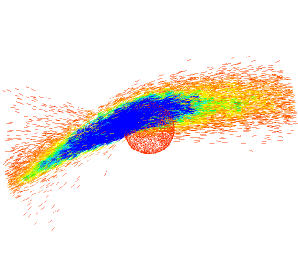
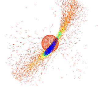
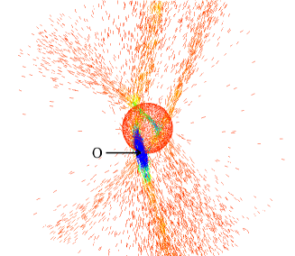
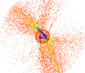
Figure 5: Snapshots of $10^{9}M_{\odot}$ clumps whose center of mass is near the surface $S$ at $t=t_{0}$ on their first (upper left) through fourth (lower right) orbits through the Galaxy. The surface $S$ is represented by the sphere in the center of each panel. Darker regions correspond to higher densities. The symbols used for the particles are elongated in the direction of their velocity. The ‘O’ in the lower left panel signifies the position of an observer used later in the discussion.

Figure 5 provides snapshots of $10^{9}M_{\odot}$ clumps that reach the solar neighborhood today on their first, second, third and fourth orbits through the Galaxy. The effects of tidal fields on the clumps are clearly evident. During the first couple of orbits, a clump is stretched into a long tidal stream which, by the third and fourth orbits, wraps around the Galaxy. However, the high density clump cores survive for many dynamical times.

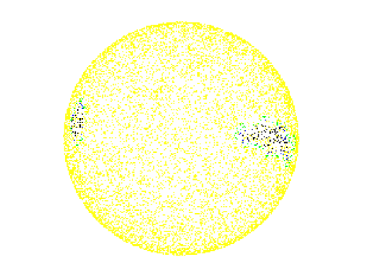
Figure 6: Sphere of observers and the density they measure as a stream passes through. Darker regions of the sphere correspond to higher measured densities.

Figure 6 illustrates what our sphere of hypothetical observers see as a clump passes through the inner part of the Galaxy for the first time. There are two distinct regions of high measured density where the clump enters and exits the $r=r_{s}$ sphere. Thus, at this instant, a small fraction of observers measure a high density of high-velocity clump particles while most of the observers measure a relatively low density of clump particles.

Figure 7 shows the measured values of $f_{n}$ as a function of $\rho$ for $10^{9}M_{\odot}$ clumps that reach the inner region of the Galaxy by the present epoch on their first, second, third, or fourth orbit. The analytic result (Eq. (20)) is shown for comparison. For clumps on their first passage through the inner region of the Galaxy, the numerical and analytic results for $f_{n}$ as a function of $\rho$ have roughly the same form. This is to be expected since tidal fields have only just started to disrupt the clump by this stage in its evolution. The analytic result underestimates the measured values by a factor $\sim 4$. This is easily understood as follows: In evaluating Eq. (20) we set $v_{r}=550\,{\,\rm km\,s^{-1}}$, the characteristic velocity of the clump at the solar radius. In fact, we should use the component of the clump velocity normal to the sphere of observers which, for orbits whose turnaround radius is comparable to $r_{s}$, is considerably less than $550\,{\,\rm km\,s^{-1}}$.

Tidal effects distort the shape of the $f_{n}$ vs. $\rho$ curve. The general trend is to increase the probability at low densities and decrease the probability at high densities, the transition occurring at $\rho=10^{-2}\rho_{B}$. Note that for very high densities, $f_{n}$ approaches the value expected from the analytic results. These regions are at the centers of the clumps where the densities are so high that they are not tidally disrupted.

Our result for $P(\rho_{D}>\rho)$, the probability that the Earth is passing through a stream of density greater than $\rho$ is shown in Figure 8. This figure indicates that there is a high probability for the Earth to be passing through a clump or stream with density $\sim 3\%$ of the mean local halo density $\rho_{B}$. The probability drops precipitously with density to values below $0.01$ for streams that would contribute a density comparable to that of the background.

The separate contributions to $dP/d\rho$ from objects on their first through fourth passages through the Galaxy are shown in Figure 9. The largest contributions come from objects that have made several passes through the Galaxy. This is primarily due to the increase in accretion rate with turnaround redshift. Additionally, clumps are stripped of particles with each passage through the Galactic center so that the tidal stream of, say a “fourth-pass clump” wraps several times around the Galaxy. Thus, the contributions to the density can come from what are essentially independent phase space streams. One might be concerned that our assumption of a spherically symmetric Galaxy potential artificially forces these streams to lie in a single plane, enhancing $dP/d\rho$ at large $\rho$. However, we are confident that our cut-off at fourth-pass clumps is sufficiently conservative that this should not be a big effect.

Finally, we turn to the velocity distribution of particles as a clump or stream passes through the observation shell $S$. The velocity space coordinates of particles within $0.5\,{\rm kpc}$ of $S$ for the four snapshots in Figure 5 ($10^{9}\,M_{\odot}$ clumps that have made $1-4$ passes through the Galaxy by the present epoch) are shown in Figure 10. On its first pass through the inner part of the Galaxy, the clump is tidally disrupted with particles spreading out along the orbit of the clump center-of-mass. In velocity space, particles have a fairly tight distribution in speed but are spread out in direction as we expect from Liouville’s theorem. By the third pass through the Galactic center, several streams are apparent and the velocity distribution becomes rather complicated.

More relevant for our purposes is the velocity space distribution as determined by a given observer. For illustrative purposes, we choose observer ‘O’ located at the instantaneous position of the center of mass for the clump in Figure 5 that has made three passes through $S$. Figure 11 shows the velocity space distribution for particles within $0.5\,{\rm kpc}$ of $O$. The distribution is anisotropic with an rms dispersion along the direction of motion of $19{\,\rm km\,s^{-1}}$ and dispersion along the two transverse directions of $34{\,\rm km\,s^{-1}}$ and $53{\,\rm km\,s^{-1}}$, again consistent with what one expects from Liouville’s theorem. A more detailed discussion of the evolution of a satellite’s velocity space distribution and the connection with Liouville’s theorem can be found in hw .

VI Experimental Signatures of Accreted Clumps and Streams

VI.1 WIMP Search Experiments

At present, over twenty groups around the world have deployed or are in the process of building terrestrial detectors designed to search for WIMPs morales . These experiments attempt to measure the energy deposited when a WIMP interacts with a nucleus in the detector. A WIMP of mass $m_{\chi}$ that scatters elastically with a nucleus of mass $m_{N}$ deposits an energy $Q=\left(m_{r}^{2}v^{2}/m_{N}\right)\left(1-\cos\theta^{*}\right)$, where $m_{r}\equiv m_{N}m_{\chi}/\left(m_{N}+m_{\chi}\right)$ is the reduced mass, $v$ is the speed of the WIMP relative to the nucleon, and $\theta^{*}$ is the scattering angle in the center-of-mass frame. The differential detection rate (per unit detector mass) can be written (e.g., jgk ):

$$\frac{dR}{dQ}=\frac{\sigma_{0}\rho_{L}}{2m_{r}^{2}m_{\chi}}G^{2}(Q)\int_{v_{\rm min}}^{\infty}F(v)\frac{dv}{v}$$ (30)

where $\sigma_{0}$ is the scattering cross-section, $\rho_{L}$ is the local WIMP density, $G(Q)$ is a form factor for the WIMP-nucleon interaction, and $v_{\rm min}=\left(Qm_{N}/2m_{r}^{2}\right)^{1/2}$. Here $F(v)$ is the normalized distribution of WIMP speeds ($\int F(v)dv=1$) in the rest frame of the detector, obtained by integrating the three-dimensional velocity distribution $f({\bf v})$ over angles.

In keeping with the discussion of the previous section, we assume that the local distribution of WIMPs can be split into a smooth background and a single coherent clump or stream, so that

$$\frac{dR}{dQ} = \frac{dR_{B}}{dQ}+\frac{dR_{C}}{dQ}$$ (31)

$$= \frac{\sigma_{0}\rho_{B}}{2m_{r}^{2}m_{\chi}}G^{2}(Q)\left(T_{B}(Q)+T_{C}(Q)\right)~{},$$ (32)

where the subscripts $B$ and $C$ refer to the background and clump respectively, and $\rho_{B}$ denotes the smooth local halo density in the absence of the clump. The remaining terms are given by

$$T_{B}(Q)=\int_{v_{\rm min}}^{\infty}F_{B}(v)\frac{dv}{v}$$ (33)

and

$$T_{C}(Q)=\frac{\rho_{C}}{\rho_{B}}\int_{v_{\rm min}}^{\infty}F_{C}(v)\frac{dv}{v}~{}.$$ (34)

A standard model for the halo background velocity distribution is the Maxwellian distribution, assumed to be isotropic in the rest frame of the Galaxy:

$$f_{B}({\bf v}^{\prime})=\frac{1}{\pi^{3/2}v_{B}^{3}}e^{-{v^{\prime}}^{2}/v_{B}^{2}}$$ (35)

where ${\bf v}^{\prime}$ is the WIMP velocity in the rest frame of the Galaxy, and $v_{B}$ is the two-dimensional halo velocity dispersion, corresponding approximately to the circular velocity at the position of Sun in the Galaxy, $v_{B}\simeq 220$ km s^-1. Let ${\bf V}_{EB}$ be the velocity of the Earth relative to the Galaxy frame (assumed to be non-rotating), so that ${\bf v}^{\prime}={\bf v}+{\bf V}_{EB}$. Transforming the distribution (VI.6) into the Earth frame (e.g., ffg ) and substituting into (VI.4) yields

$$T_{B}(Q)=\frac{1}{2V_{EB}}\left({\rm erf}{\left(\frac{V_{EB}+v_{\rm min}}{v_{B}}\right)}+{\rm erf}{\left(\frac{V_{EB}-v_{\rm min}}{v_{B}}\right)}\right)$$ (36)

In what follows, we use a slightly more complicated expression that assumes a velocity-space cut-off at the escape speed of the Galaxy with the value $v_{\rm esc}=575\,{\,\rm km\,s^{-1}}$ (e.g., ffg ). If we assume that the velocity distribution of the WIMPs in a clump is Maxwellian and isotropic in the rest frame of the clump, with internal velocity dispersion $v_{C}$, then

$$T_{C}(Q)=\frac{\rho_{C}}{2\rho_{B}V_{EC}}\left({\rm erf}{\left(\frac{V_{EC}+v_{\rm min}}{v_{C}}\right)}+{\rm erf}{\left(\frac{V_{EC}-v_{\rm min}}{v_{C}}\right)}\right)~{}$$ (37)

where $V_{EC}$ is the relative velocity of the Earth and the clump.

It is straightforward to understand heuristically the effect of a WIMP clump on the nuclear recoil energy spectrum in a dark matter detector. The key observation is that the clump internal velocity dispersion $v_{C}\sim 50\,{\,\rm km\,s^{-1}}$, is small compared to $V_{EC}\sim 525$ km s^-1. In the limit $v_{C}/V_{EC}\rightarrow 0$, the clump particle distribution function in the frame of the Earth is given by $F_{C}(v)\propto\delta(v-V_{EC})$; from (VI.1), this implies that the detection rate is constant, with an amplitude proportional to $1/V_{EC}$, if $V_{EC}>v_{\rm min}(Q)$ and zero otherwise. That is, the detection rate is constant at small $Q$, and zero beyond some maximum value $Q_{\rm max}=2m_{r}^{2}V^{2}_{EC}/m_{N}$. The value of $Q_{\rm max}$ varies seasonally, as the Earth’s velocity relative to the clump changes. Including the non-zero clump velocity dispersion $v_{C}$ turns this sharp cutoff in the detection rate into a smooth shoulder, with a width proportional to $v_{C}$.

As discussed above, the distribution of particles in velocity space for a tidally disrupted clump is anisotropic. In particular, the dispersion is a factor of $2-3$ times smaller along the orbit of the clump (defined by ${\bf V}_{CB}$, the velocity of the clump in the Galaxy frame) as compared with the transverse directions (cf. Figure 11). $F_{C}(v)$ is calculated in the Earth frame of reference (in Figure 10, the distribution of $v$ about a point displaced from the origin by $V_{EB}$). The width of the peak of $F_{C}(v)$ therefore depends on the angle between ${\bf V}_{EB}$ and ${\bf V}_{CB}$. When these velocities are colinear, the distribution is relatively narrow. When they are close to perpendicular, the distribution is somewhat broader. In either case, the dispersion in $v$ is small compared with the dispersion of particles in the background. Thus, velocity space anisotropy alters the detailed shape of the feature in a recoil spectrum but not its general characteristics. While it is straighforward to include velocity space anisotropy in the calculations that follow, doing so increases the number of parameters and complicates the discussion. Therefore we work under the assumption that the clump velocity dispersion is isotropic.

The recoil energy spectra for $V_{EC}=401,\,569,\,$ and $698\,\,{\,\rm km\,s^{-1}}$ are shown in Figure 12. These velocities correspond to a clump moving with a speed of $V_{CB}=525\,{\,\rm km\,s^{-1}}$ relative to the Galaxy at an angle with respect to ${\bf V}_{EB}$ of $45^{\circ},\,90^{\circ},\,135^{\circ}$, respectively. For ${\bf V}_{EB}$ we use the Sun’s velocity relative to the Galaxy (seasonal modulation will be discussed below). In this example, we have assumed a clump with local density equal to $3\%$ of the local halo density, i.e., $\rho_{C}=9\times 10^{-3}$ GeV cm^-3 at the position of the Earth, which Fig. 8 shows to be a common occurence. $dR/dQ$ is given in units of Events per kg of detector per ${\rm keV}$ per day with assumed parameters $\sigma_{0}=4\times 10^{-36}\,{\rm cm}^{2}$, $m_{\chi}=50\,{\rm GeV}$ and $m_{N}=68.5\,{\rm GeV}$ corresponding to a ⁷³Ge detector. In addition, we have set the nuclear form factor $G(Q)=1$. As anticipated, the contribution from the clump is well-approximated by a step function in $Q$ with a more pronounced contribution from the clump at larger values of $V_{EC}$. Though the number of events per energy bin decreases as $1/V_{EC}$, the total number of events increases as $V_{EC}$. A positive feature of the clump signal, in terms of detectability, is that it dominates over the background halo signal at high recoil energy, where radioactive backgrounds are generally small. A negative feature is that the absolute detection rate associated with a clump is not likely to be large (which is why it is subdominant at lower energies), so a large total detector mass would be necessary.

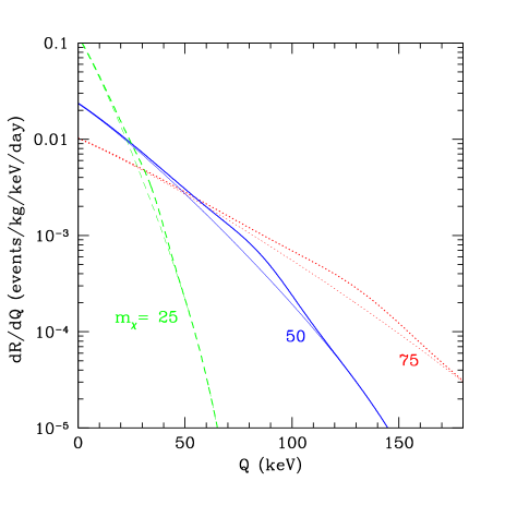
Figure 13: Theoretical differential event rate for WIMP masses $m_{\chi}=25\,{\rm GeV}$ (dashed line), $m_{\chi}=50\,{\rm GeV}$ (solid line), and $m_{\chi}=75\,{\rm GeV}$ (dotted line). Other parameters are the same as in Figure 12.

Figure 13 shows recoil spectra for various WIMP masses. The background spectra exhibit the usual dependence with $m_{\chi}$: spectra for smaller $m_{\chi}$ fall off faster with $Q$. Likewise, the clump feature moves to higher energies as $m_{\chi}$ is increased.

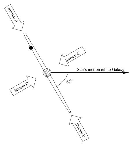
Figure 14: Various stream directions as viewed in the rest frame of the solar system. Also shown is the Sun and its direction of motion around the Galactic center and the Earth and its orbit around the Sun. Spectral features due to Streams A and B will have the maximum seasonal modulation while Streams C and D will show no seasonal modulation. The modulation of the feature due to Stream B (A) will be in phase ($180^{\circ}$ out of phase) with that of the background.

While the hierarchical model gives statistical predictions for the clump density, velocity, and velocity dispersion, the seasonal variation of the signal depends on the relative velocity of the clump and the Sun, which we cannot predict a priori. Figure 14 shows several choices for the clump or stream velocity vector. The direction of motion of the Sun around the galaxy and the orbit of the Earth around the Sun (the plane of which is perpendicular to the page) are also shown. The Earth is at the upper left point of its orbit on about June 2 and at the lower right six months later. For directions A or B, the annual modulation of the clump signal, that is, the amplitude of the yearly variation in the maximum recoil energy $Q_{\rm max}$, is maximal, of order 25% peak to peak; for streams C and D, perpendicular to Earth’s orbit, there is no seasonal modulation of the clump signal. For stream A, $Q_{\rm max}$ reaches a minimum on June 2 and a maximum six months later; for stream B, the situation is reversed. Note that the four directions shown here all lie in the plane defined by the Sun’s velocity and the orbital axis of the Earth around the Sun. In such cases, the annual modulation of the clump signal is in phase (or anti-phase) with the annual modulation of the background halo (which is set by the relative velocity of the Earth with respect to the Galactic halo), with a peak or trough on June 2. We emphasize that this is a special case: in general, the clump orbit will not lie in this plane and will therefore have a different phase from that of the smooth background halo. Consequently, the phase of the clump signal modulation constrains the clump direction of motion.

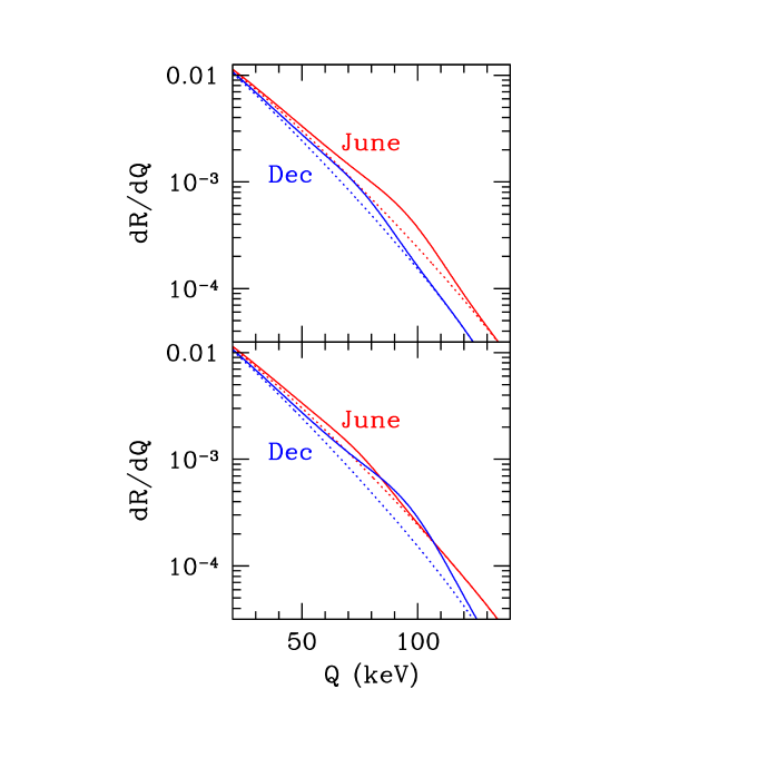
Figure 15: Theoretical event rate vs. deposited energy for June (red lines) and December (blue lines). Dotted lines are the signal from the background; solid lines are the signal from background plus 3% clump. Top panel: modulation of stream and background are in phase (stream B from Figure 14). Bottom panel: modulation of stream and background are $180^{\circ}$ out of phase (stream A from Figure 14).

Figure 15 shows the seasonal modulation for example B of Figure 14. The two solid lines show the shifts in the spectrum due to seasonal variation of the clump signal, while the seasonal modulation of the background signal ffg is shown by the two sets of dotted curves. The fractional modulation signal,

$${\cal F}(Q)=\frac{\left(dR/dQ\right)_{\rm June}-\left(dR/dQ\right)_{\rm Dec}}{\left(dR/dQ\right)_{\rm June}+\left(dR/dQ\right)_{\rm Dec}}$$ (38)

is shown in Figure 16 for both B (clump feature and background in phase) and A (feature and background out of phase).

If the recoil spectral feature due to the clump can be detected, then it should be possible in principle to determine the physical parameters of the dark matter stream: its density, direction of origin, velocity, and velocity dispersion. The maximum recoil energy associated with the clump $Q_{\rm max}$ determines the product $m_{r}V_{EC}$. The background halo signal itself determines $m_{r}v_{B}$; if $v_{B}$ is sufficiently reliably determined from the galaxy rotation curve, then $V_{EC}$ can be extracted. The clump velocity dispersion $v_{C}$ is then determined from the width of the clump recoil shoulder near $Q=Q_{\rm max}$, and the clump density $\rho_{C}$ from the relative amplitude of the clump and background halo signals. Finally, the phase of the clump modulation signal constrains the plane of the clump orbit, while the amplitude of the clump modulation signal, along with the parameters above, constrains the direction of the clump velocity vector in that plane. In practice, of course, given finite detector energy resolution, the presence of radioactive backgrounds, low counting rates, and possible confusion due to more than one clump, the dynamical information that will be extracted is likely to be more limited.

A new generation of WIMP detectors with directional sensitivity (e.g., DRIFT drift ) is now under development. The ability to measure the nuclear recoil direction would provide a new avenue for constraining the clump speed and direction relative to the Sun. Fig. 17 shows the angular recoil spectra for two special cases: clump travelling through the Halo in the same direction as the Sun and clump travelling in the opposite direction from the Sun. In each case, we assume that the clump speed in the Galactic rest frame is $525{\,\rm km\,s^{-1}}$. We choose a clump dispersion $v_{C}=25{\,\rm km\,s^{-1}}$ which is a factor of two smaller than what was used in the previous discussion. (Recall that the velocity dispersion is smaller along the direction of motion of the clump than in the two transverse directions. Since we are considering the special case where clump and solar system velocities are colinear, we select a dispersion at the low end of the expected range.) When the WIMP stream is travelling in the same direction as the Sun there is an increased probability of forward scattering. When the stream travels against the sun’s motion, rearward scattering is increased. Note that there is an appreciable signal when clump and Sun are moving in the same direction whereas the feature in the energy spectrum for this case is barely detectable.

VI.2 Axion Search Experiments

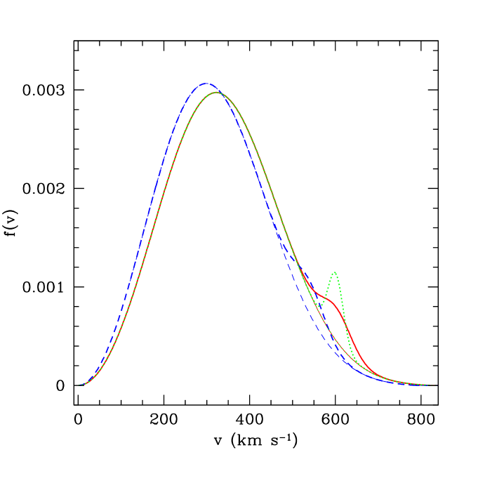
Figure 18: Speed distribution for Maxwellian background (light lines), and clump plus background (heavy lines). Shown are distribution functions for June (solid lines) and December (dashed lines) assuming seasonal modulation of clump and background are in phase (Stream B in Figure 14) and a clump velocity dispersion $v_{C}=50{\,\rm km\,s^{-1}}$. Also shown is the distribution function for June assuming a velocity dispersion of $25{\,\rm km\,s^{-1}}$ (dotted). A clump speed relative to the Sun of $569{\,\rm km\,s^{-1}}$ was chosen.

Axions are pseudo-scalar particles that arise in theories designed to solve the Strong CP problem (e.g., kim ). Although in most models these particles are extremely light, in the early Universe, they are non-relativistic and therefore behave like other cold dark matter candidates. The direct detection scheme for these particles relies on their coupling to photons ($a\gamma\gamma$) hagmann ; sikivie . In a magnetic field, the axion can convert into a microwave photon with an energy equal to the axion’s total (rest mass plus kinetic) energy; this signal can be detected with a suitably tuned microwave cavity. In this respect, axions would provide a more direct picture of the distribution function of dark matter. The axion energy spectrum in Figure 18 shows that significant features can be introduced into the spectrum (thick lines) which are not present in the pure Maxwellian background model (thin lines). Here, we have assumed the same parameters as in our discussion of WIMP detection via nuclear recoil ($v_{C}\sim 50{\,\rm km\,s^{-1}},\,V_{EC}=569{\,\rm km\,s^{-1}},\,\rho_{C}/\rho_{B}=0.03$). The feature appears as a platueau at high velocities, right where the background is dropping rapidly. Moreover, if the clump dispersion is smaller, the feature appears as a distinct secondary peak. This is illustrated by the dotted curve where we assume $v_{C}=25{\,\rm km\,s^{-1}}$.

By following the motion of the secondary peak throughout the course of a year, considerable additional information about the dynamics of the stream can be determined. The range of velocities over which the peak moves corresponds to the angle of the stream with respect to the plane of the Earth’s orbit. For example, a stream perpendicular to the Earth’s orbit would show no variation over the course of a year while one parallel would show the maximum variation. The phase of the seasonal modulation in the position of the peak can be used to determine the azimuthal direction of the stream as well. This would give a complete dynamical description of the stream. Since the axion detection spectrum gives direct access to the axions’ energy distribution, it is likely easier to determine the stream parameters than for the case of WIMPs.

VII Conclusion

Dark matter detection experiments may provide a new window to the Universe. If successful, the results would have dramatic implications for the field of particle physics, leading to physics beyond the Standard Model. The implications for cosmology would be equally important since dark matter represents $\sim 30\%$ of the energy density of the Universe and $\sim 90\%$ of the mass in gravitationally bound structures. The results presented here suggest that dark matter search experiments can also provide clues to the formation history of the Galactic halo.

Most analyses of direct detection experiments take, as a starting point, the assumption that the velocity-space distribution of dark matter particles in the solar neighborhood is smooth and approximately Maxwellian. However, N-body simulations indicate that CDM halos have a high degree of substructure due to undigested lumps and tidal streams. To what extent can this substructure affect the results of dark matter detection experiments? Current N-body simulations do not have the resolution to answer this question moore2001 . It is for this reason that we have developed a hybrid approach based on the extended Press-Schecter formalism and N-body simulations of individual clumps evolving in a background potential.

Our main results are summarized in Figure 8. Taken at face value, they imply that there is a high probability for the local density of dark matter particles to be enhanced by a clump or stream with a density equal to $\sim 3\%$ of the background. The probability drops precipitously as a function of clump density and is negligible for densities comparable to that of the background.

A dynamically ‘cold’ dark matter stream with a density $\sim 3\%$ of the background can produce an observable feature in the energy or angular spectra of a terrestrial search experiment. For recently accreted clumps and their associated tidal streams, the anticipated features appear at high energies precisely where the signal from the background drops dramatically. In addition, the seasonal modulation of the stream’s signal will be different from that of the background. In principle, energy and angular spectra would allow one to extract various clump parameters such as its internal velocity dispersions, and velocity (speed and direction) relative to the Earth. We conclude by noting that this model of halo substructure could yield other observable detection signatures that would be interesting to explore — for example, in events arising from WIMP annihilations in the cores of accreted clumps.

Figure 1: Schematic illustration of the change in variables from $z_{\rm ta}$ to $t$ used in evaluating $dP/d\rho$. Top: six orbits that reach different radii at $t=t_{0}$. Bottom: two orbits used to approximate the contributions bracketed by orbits $a-c$ and $d-f$ of the top panel.

Figure 2: Three realizations of the growth of a $2\times 10^{12}M_{\odot}$ dark halo. The heavy straight line is the analytic fitting formula $M(t)=M_{0}(t/t_{0})^{1.5}$ used to calculate $dP/d\rho$.

Figure 3: Initial condition parameter space and corresponding orbits. Left: $r_{\rm ta}-J$ parameter space for orbits that are near the surface $S$ at $t=t_{0}$. The strips of points at $r_{\rm ta}=380,285,230$, and $195$ kpc correspond to particles that reach $S$ after $1,\,2,\,3$ or $4$ orbits through the Galaxy respectively. The large dots are the initial conditions used in the numerical simulations. Right: Distance from the Galactic center as a function of time for the orbits shown in the left panel.

Figure 4: Density profiles for Hernquist (solid curve) and NFW (dashed curve) models assuming a virial mass, $10^{9}M_{\odot}$. The shaded region corresponds to densities at the detector of $\rho=10^{-3}\rho_{B}-10^{-1}\rho_{B}$ where $\rho_{B}=6\times 10^{4}\rho_{\rm crit}$ is the density of dark matter particles in the background.

Figure 7: The quantity $f_{n}$ as a function of density for $10^{9}\,M_{\odot}$ clumps that reach $S$ at $t=t_{0}$ on their first through fourth orbits through the Galaxy. Solid lines show the analytic results assuming no tidal disruption while the symbols show the results obtained from the numerical simulations. The two types of symbols correspond to two different choices of orbital angular momentum shown in Figure 3 — crosses are the higher angular momentum, triangles are the lower angular momentum.

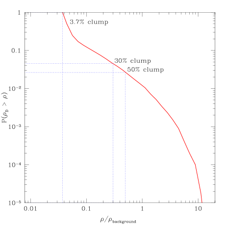
Figure 8: Probability for the Earth to be passing through a stream with local density greater than $\rho$. $\rho$ is given in units of the background density, $\rho_{B}=0.3\ {\rm GeVcm}^{-3}=8\times 10^{-3}\ M_{\odot}{\rm pc}^{-3}$.

Figure 9: Contribution to $dP/d\ln\rho$ from objects on their first through fourth pass through $S$ (lower line through to upper line respectively).

Figure 10: Distribution in velocity space of particles within $0.5\,{\rm kpc}$ of the observer shell $S$ for clumps on their first through fourth orbit through the Galaxy. Particle distributions are the same as in Figure 5. Velocities are projected onto the orbital ($xy$) plane.

Figure 11: Three projections of the velocity space distribution of particles within $0.5\,{\rm kpc}$ of the observer ‘O’ that is indicated in the lower left panel of Figure 5. Velocities are given in ${\,\rm km\,s^{-1}}$.

Figure 12: Theoretical differential event rate per kg per keV per day as a function of recoil energy for different clump speeds as measured in the rest frame of the Earth. The clump speeds are, from left to right, $401,\,569,\,$ and $698{\,\rm km\,s^{-1}}$ corresponding to a clump moving through the Galaxy with $V_{CG}=525{\,\rm km\,s^{-1}}$ at angles relative to ${\bf V}_{EB}$ of $45^{\circ},\,90^{\circ}\ {\rm and}\ 135^{\circ}$ respectively. The dotted, dashed, and solid lines are the detection rates due to the background, the clump and the clump plus background respectively. Parameters chosen for the calculation are $\rho_{C}/\rho_{B}=0.03$, $\sigma_{0}=4\times 10^{-36}{\rm cm}^{2}$, $G(Q)=1$, $m_{\chi}=50\,{\rm GeV}$, and $m_{N}=68.5\,{\rm GeV}$.

Figure 16: Fractional modulation signal ${\cal F}(Q)$ as defined in Eq. (38) vs.  $Q$ The solid line shows the result for the background. The dashed line shows the result for background plus stream B of Figure 14 (modulation signal of stream in phase with that of background). The dotted line shows the result for background plus stream A (modulation signal of stream $180^{\circ}$ out of phase with that of background).

Figure 17: Relative event rate as a function of recoil angle for a Maxwellian background (dotted line), a 3% clump (dashed line), and clump plus background (solid line). $\theta=0$ corresponds to a recoil event in the direction opposite to that of the Sun’s motion around the Galaxy. Velocity of clump and Sun are assumed to be colinear. Left: Clump moving in the same direction as the Sun. Right: Clump moving opposite to the Sun. Clump speed in the rest frame of the Galaxy is $525{\,\rm km\,s^{-1}}$. Other parameters are the same as in the previous Figures.