Quintessential Haloes around Galaxies

Abstract

The nature of the dark matter that binds galaxies remains an open question. The favored candidate has been so far the neutralino. This massive species with evanescent interactions is now in difficulty. It would actually collapse in dense clumps and would therefore play havoc with the matter it is supposed to shepherd. We focus here on a massive and non–interacting complex scalar field as an alternate option to the astronomical missing mass. We investigate the classical solutions that describe the Bose condensate of such a field in gravitational interaction with matter. This simplistic model accounts quite well for the dark matter inside low–luminosity spirals whereas the agreement lessens for the brightest objects where baryons dominate. A scalar mass $m\sim 0.4$ to $1.6\times 10^{-23}$ eV is derived when both high and low–luminosity spirals are fitted at the same time. Comparison with astronomical observations is made quantitative through a chi–squared analysis. We conclude that scalar fields offer a promising direction worth being explored.

11 September 2001

I Introduction.

The observations of the Cosmic Microwave Background anisotropies [1] point towards a flat universe. The determination of the relation between the distance of luminosity and the redshift of supernovae SNeIa [2] strongly favors the existence of a cosmological constant which contributes a fraction $\mbox{$\Omega_{\Lambda}$}\sim 0.7$ to the closure density. The pressure–to–density ratio $w$ of that fluid is negative with a value of $w=-1$ in the case of an exact cosmological constant. Alternatively, this component could be in the form of dark energy – the so–called quintessence – whose simplest incarnation is a neutral scalar field $\Phi$ with the Lagrangian density

$${\cal L}\;=\;\frac{1}{2}\,g^{\,\mu\nu}\,\partial_{\mu}\Phi\,\partial_{\nu}\Phi\,-\,V\left(\Phi\right)\;\;.$$ (1)

Should the metric be flat and the field homogeneous, the energy density may be expressed as

$$\rho\equiv T^{0}_{\;0}\;=\;{\displaystyle\frac{\dot{\Phi}^{2}}{2}}\,+\,V\left(\Phi\right)\;\;,$$ (2)

whereas the pressure obtains from $T_{ij}\equiv-g_{\,ij}\,P$ so that

$$P\;=\;{\displaystyle\frac{\dot{\Phi}^{2}}{2}}\,-\,V\left(\Phi\right)\;\;.$$ (3)

If the kinetic term is negligible with respect to the contribution of the potential, a pure cosmological constant – $\omega=-1$ – is recovered. Cosmological scenarios with quintessence in the form of a scalar field have been investigated [3] with various potentials and their relevance to structure formation has been discussed.

On the other hand, matter contributes a fraction $\mbox{$\Omega_{\rm M}$}\sim 0.3$ to the energy balance of the universe. The nature of that component is still unresolved insofar as baryons amount only to [4]

$$\mbox{$\Omega_{\rm B}$}\,h^{2}\;=\;0.02\pm 0.002\;\;.$$ (4)

According to the common wisdom, non–baryonic dark matter would be made of neutralinos – a massive species with weak interactions that naturally arises in the framework of supersymmetric theories. This approach has given rise to some excitement in the community and many experimental projects have been developed to hunt for these evading particles. The general enthusiasm has been recently refreshed when numerical simulations have shown that cold dark matter would cluster in very dense and numerous clumps [5] (see however [6]). The halo of the Milky Way should contain $\sim$ half a thousand satellites with mass in excess of $10^{8}$ $M_{\odot}$ while a dozen only of dwarf–spheroidals are seen. The clumps would also heat and eventually shred the galactic ridge. More generally, this process would lead to the destruction of the disks of spirals. A neutralino cusp would form at the centers of the latter. This is not supported by the rotation curves of low surface brightness galaxies that indicate on the contrary the presence of a core with constant density. Finally, two–body interactions with halo neutralinos and its associated dynamical friction would rapidly disrupt the otherwise observed spinning bar at the center of the Milky Way.

Neutralinos may be in jeopardy. New candidates are under scrutiny such as particles with self interactions [7]. An interesting possibility is based on configurations of the above–mentioned scalar field $\Phi$ for which the pressure $P$ vanishes. An academic example is provided by the exponential potential

$$V\left(\Phi\right)\;=\;\frac{1}{2}\,\rho^{0}_{\Phi}\,\exp\left\{-\beta\left(\Phi_{0}-\Phi\right)\right\}\;\;,$$ (5)

where the parameter $\beta$ is

$$\beta\;=\;{\sqrt{\displaystyle\frac{24\,\pi\,G}{\Omega_{\Phi}}}}\;\;.$$ (6)

In a flat and matter–dominated universe, such a field $\Phi$ would behave just exactly as cold dark matter and would contribute a fraction $\Omega_{\Phi}=\rho^{0}_{\Phi}/\rho^{0}_{C}$ to the closure density. More generally, the kinetic energy ${\dot{\Phi}^{2}}/{2}$ should cancel the potential $V\left(\Phi\right)$ in order for the pressure to vanish and for the fluid to mimic the effect of non–relativistic matter. As will be discussed in the next section, this is actually the case when $\Phi$ behaves like an axion and oscillates coherently on a time scale much shorter than the typical durations at stake. Alternatively, the field $\Phi$ could have additional degrees of freedom and rotate in the corresponding internal space. The idea that the excess of gravity inside galaxies may be due to a classical configuration of some scalar field $\Phi$ has already drawn some attention. The discussion has nevertheless remained at an introductory level. A condensate of massive bosons with repulsive interparticle potential has been postulated [8] to suppress the formation of structure on subgalactic scales. The polytropic index of this bosonic halo varies from $n=1$ at low density up to $n=3$ at high density. The stability and annihilation of such a system has been mentioned in [9] and a limit on the quartic coupling constant of $\Phi$ has been derived. The relevance of scalar fields to the structure of galactic haloes and their associated dark matter cannot be seriously addressed without comparing the theoretical rotation curves to the observations. An exponential potential – with negative overall sign – is shown [10] to lead to flat rotation curves. A massless and non–interacting complex scalar field is thoroughly considered in [11]. The self–gravitating structure of the field is calculated.

We nevertheless feel that these analysis may be improved in several ways. To commence, a negative potential does not seem quite appealing. It actually leads to unphysical situations where the scalar field rolls down the hill indefinitely and converts the infinite amount of energy stored into $V<0$ into kinetic energy. Then, as mentioned in [12], the rotation curves are assumed to be flat up to an infinite distance. In both [10] and [11], the Bose condensate extends to infinity and the mass of the system diverges linearly in the radius $r$. The Minkowski metric is no longer recovered at large $r$. On the contrary, space exhibits a small deficit of solid angle. We feel that such a behavior is not realistic insofar as the rotation curves of bright spirals are actually found to decrease beyond their optical radius [13]. Another strange consequence is that Newton’s gravitation does not apply even when the fields are weak. Matching the metric with the Robertson–Walker form may also be a problem. Finally, the agreement between the predicted and the observed rotation curves is only qualitative and in the case of [10] is based on just a few examples. The goodness of that agreement is not assessed from a quantitative point of view.

This motivated us to reinvestigate more thoroughly the subject. In the next section, we discuss the general conditions under which a scalar field may bind galaxies. We show that the same field cannot easily account – at the same time – for the dark matter at galactic scales and for the cosmological quintessence. We explain the reasons which have lead us to consider the model scrutinized in section III. The corresponding rotations curves are derived in section IV and are compared by means of a chi–squared analysis to the universal curves unveiled by [13]. The results are discussed in section V and prospects for future investigations are finally suggested.

II Can a scalar field bind galaxies ?

In the weak field approximation of general relativity – or quasi–Newtonian limit – deviations from the Minkowski metric $\eta_{\mu\nu}={\rm diag}(1,-1,-1,-1)$ are accounted for by the perturbation $h_{\mu\nu}$. In the harmonic coordinate gauge where it satisfies the condition

$$\partial_{\alpha}h^{\alpha}_{\;\mu}\,-\,\frac{1}{2}\partial_{\mu}h^{\alpha}_{\;\alpha}\;=\;0\;\;,$$ (7)

this perturbation $h_{\mu\nu}$ is related to the source tensor

$$S_{\mu\nu}\;=\;T_{\mu\nu}\,-\,\frac{1}{2}\,g_{\mu\nu}\,T^{\alpha}_{\;\alpha}\;\;.$$ (8)

through

$$h_{\mu\nu}\left(\vec{r}\right)\;=\;-\,4\,G\;{\displaystyle\int}\,{\displaystyle\frac{S_{\mu\nu}\left(\vec{r}\,^{\prime}\right)}{|\,\vec{r}\,^{\prime}\,-\,\vec{r}\,|}}\,d^{3}\vec{r}\,^{\prime}\;\;.$$ (9)

The stress–energy tensor is denoted by $T_{\mu\nu}$. The gravitational potential – which in the quasi–Newtonian approximation is nothing but $h_{00}/2$ – is sourced by $S_{00}$. Note that in the case of pressureless matter, one would have $2S_{00}=T_{0}^{0}$ and the gravitational potential would just be sourced by the energy density. So, the scalar field generates the same gravitational potential as an equivalent cold matter component with energy density $2S_{00}$. For this reason, the later quantity can be called the effective density. In the simplest case of the neutral scalar field $\Phi$ of Eq. (1), it reads:

$$\rho_{\rm eff}\equiv 2S_{00}\;=\;2\left(\partial_{0}\Phi\right)^{2}\,-\,2V\;\;.$$ (10)

Note that unlike the true energy density, $\rho_{\rm eff}$ contains no space–derivatives $\partial_{i}\Phi$.

In order to generate the gravitational potential well that is observed inside galaxies, a distribution of dark matter is generally introduced in addition to the baryon population. An excess of binding ensues and matter is tied more closely. Should the scalar field $\Phi$ be responsible for the haloes of galaxies, its effective density $\rho_{\rm eff}$ would play the role of the ordinary cold dark matter density, and should in particular be positive. Since the gravitational potential in a galaxy is essentially static, we would have to assume – a priori – that the time derivative $\dot{\Phi}=\partial_{0}\Phi$ vanishes. The effective density $\rho_{\rm eff}$ would therefore reduce to $-\,2\,V\left(\Phi\right)$ and the field potential would have to be negative. This is actually the solution suggested by [10]. However, even if we are not aware of a principle that strictly forbids a negative potential, we would prefer to avoid such an unusual assumption. Nothing would prevent the system from being unstable in that case and we will therefore disregard this option. On the other hand, a static field with positive potential $V$ leads to a positive Newtonian potential and therefore to repulsion. It would lessen the attraction of ordinary matter and disrupt galaxies. This is not completely surprising since the same positive $V$ is proposed to accelerate the expansion of the universe as its contents repel each other. This property has led to the hasty conclusion that a scalar field could not bind matter inside galaxies.

Let us assume however that the scalar field $\Phi$ varies much more rapidly than the system in which it is embedded. Our Milky Way rotates in $\sim$ 200 million years. If the field changes on a much shorter timescale, the associated effective density would be felt through its time average

$$\rho_{\rm eff}\;=\;2\left<\dot{\Phi}^{2}\right>\,-\,2\left<V\right>\;\;.$$ (11)

The field $\Phi$ may oscillate for instance at the bottom of the potential well. The pulsation of the corresponding vibrations is equal to the scalar mass $m$ and may be derived from the curvature of the potential at its minimum in $\Phi=0$

$$m^{2}\equiv V^{\prime\prime}(0)\;\;.$$ (12)

Actually the field behaves just like an ordinary harmonic oscillator whenever the pulsation $m$ is much larger than the wavevector $k$ of the self–gravitating configuration. This translates into the condition

$${\displaystyle\frac{2\,\pi}{m}}<<R\;\;,$$ (13)

where $R$ is the typical length on which $\Phi$ changes appreciably. For the haloes of galaxies, $R$ is of order a few kpc. Because $\Phi$ varies in time like $\exp\left(-\,i\,m\,t\right)$, the kinetic and potential energies are related on average by

$$\left<V\left(\Phi\right)\right>\;=\;\left<{\displaystyle\frac{\dot{\Phi}^{2}}{2}}\right>\;\;.$$ (14)

The effective density may now induce a gravitational attraction insofar as

$$\rho_{\rm eff}\;=\;2\,\left<V\right>>0\;\;.$$ (15)

Allowing the field $\Phi$ to vibrate quickly has led to an overall change of sign with respect to the case considered in [10]. Notice furthermore that the associated pressure vanishes as a result of (3) and (14) so that the scalar fluid behaves just like non–relativistic matter. Such coherent oscillations have already been considered in the literature, in the case of the axion in particular – see also the interesting discussion of a quintessence field with a late oscillatory stage in [14].

Another illustration of a fast evolving field is to make it rotate in some internal space. We may look for configurations where the dark energy itself – and not its time–average – is rigorously static. A complex field with a uniformly rotating phase features the simplest realization of that idea

$$\Phi\;=\;{\displaystyle\frac{\sigma(r)}{\sqrt{2}}}\,e^{\displaystyle-i\,\omega t}\;\;.$$ (16)

If the field is non–interacting but has a mass $m$, the associated effective density obtains from

$${\displaystyle\frac{\rho_{\rm eff}}{2}}\;=\;S_{00}\;=\;2\,\dot{\Phi}^{\dagger}\dot{\Phi}\;-\;U\left(\Phi\right)\;\;,$$ (17)

where the potential $U=m^{2}\,\Phi^{\dagger}\,\Phi$. The pressure of the scalar fluid may be approximated by

$$P\simeq\dot{\Phi}^{\dagger}\dot{\Phi}\,-\,U\left(\Phi\right)\;\;,$$ (18)

when the space–derivatives of the field are negligible. This amounts to assume once again that the typical length $R$ of the system way exceeds $1/\omega$. Whenever the condition $m\simeq\omega$ holds, the pressure is vanishingly small and the scalar fluid behaves as a non–relativistic component. The associated effective density becomes $\rho_{\rm eff}=\omega^{2}\sigma^{2}(r)$ with no explicit dependence on the time. The complete model will be discussed in the next section where we will consider the possibility of a boson–star like system extending over a whole galaxy and playing the role of a dark halo.

We conclude this section by pointing out the difficulty to have a common explanation for both the local dark matter and the cosmological quintessence in terms of a scalar field. An excess of gravitational binding on galactic scales requires the condition

$$\dot{\Phi}^{2}\geq V\left(\Phi\right)$$ (19)

to be fulfilled. Conversely, should the overall pressure $P$ be negative to account for a cosmological constant, the potential would have to satisfy the inequality

$${\displaystyle\frac{\dot{\Phi}^{2}}{2}}\leq V\left(\Phi\right)\;\;.$$ (20)

We conclude that the pressure–to–density ratio $w$ must exceed the value of $-1/3$ in order for both conditions to be simultaneously met. Such a range seems to be already excluded by the measurements of supernovae SNeIa [2].

III The self–gravitating complex and massive scalar field.

Boson stars have been extensively studied in the past – see for instance [15, 16, 17, 18]. For clarity, we will briefly summarize the main features of self–gravitating bosons, following closely the presentation of [16]. We are interested in the stable and bounded configurations of a complex scalar field obeying the action

$${\cal S}\;=\;{\displaystyle\int}\,\sqrt{-g}\;d^{4}x\;{\cal L}\left\{\Phi,\partial_{\mu}\Phi\right\}\;=\;{\displaystyle\int}\,\sqrt{-g}\;d^{4}x\;\left\{g^{\mu\nu}\,\partial_{\mu}\Phi^{\dagger}\,\partial_{\nu}\Phi\;-\;U\left(\Phi\right)\right\}\;\;,$$ (21)

where the potential $U$ is invariant under the global symmetry

$$\Phi\longrightarrow\Phi^{\prime}=e^{\displaystyle i\alpha}\,\Phi\;\;.$$ (22)

The conservation of the corresponding conserved current is crucial for the stability of the boson star. Real scalar fields have no stable bounded configurations. One can show that all spherically symmetric minimum energy solutions depend on time only through a rotating phase so that the complex field $\Phi$ may be expressed as in Eq. (16) – see for instance the appendix in [16]. In analogy with the hydrogen atom, such solutions correspond to the energy eigenstates $(n,l=0,m=0)$. We will see later how the discrete energy levels $n$ of a boson star are associated with different values of the rotation parameter $\omega$. The parametrization (16) of $\Phi$ is compatible with a static isotropic metric

$$d\tau^{2}\;=\;e^{\displaystyle 2u}\,dt^{2}\,-\,e^{\displaystyle 2v}\,\left\{dr^{2}+r^{2}d\theta^{2}+r^{2}\sin^{2}\theta\,d\varphi^{2}\right\}\;\;,$$ (23)

where $u$ and $v$ depend only on the radius $r$. The Klein-Gordon equation reads

$$e^{\displaystyle-2v}\,\left\{\sigma^{\prime\prime}\,+\,\left(u^{\prime}+v^{\prime}+\frac{2}{r}\right)\,\sigma^{\prime}\right\}\;+\;\omega^{2}e^{\displaystyle-2u}\,\sigma\;-\;U^{\prime}(\sigma)\;=\;0\;\;.$$ (24)

The Einstein equations provide two additional independent equations of motion. We can choose for instance

$$2v^{\prime\prime}\,+\,v^{\prime 2}\,+\,\frac{4v^{\prime}}{r}\;=\;-\,8\,\pi\,G\;e^{\displaystyle 2v}\,\left\{W\;+\;V\;+\;U\right\}\;\;,$$ (25)

and

$$u^{\prime\prime}\,+\,v^{\prime\prime}\,+\,u^{\prime 2}\,+\,\frac{1}{r}\left(u^{\prime}+v^{\prime}\right)\;=\;8\,\pi\,G\;e^{\displaystyle 2v}\,\left\{W\;-\;V\;-\;U\right\}\;\;,$$ (26)

where the kinetic and gradient contributions to the field energy density are respectively denoted by

$$W\;=\;e^{\displaystyle-2u}\,{\displaystyle\frac{\omega^{2}\sigma^{2}}{2}}\qquad{\rm and}\qquad V\;=\;e^{\displaystyle-2v}\,{\displaystyle\frac{\sigma^{\prime 2}}{2}}\;\;.$$ (27)

From the assumption that boson stars are non singular configurations, asymptotically flat and of finite energy, severe restrictions can be put on the boundary conditions for $u$, $v$ and $\sigma$. In order to avoid any singularity at the origin, the radial derivatives $u^{\prime}$, $v^{\prime}$ and $\sigma^{\prime}$ must vanish at $r=0$. Actually, since an angular deficit at the origin would imply an infinite concentration of energy, we infer the complementary condition $v(0)=0$. This appears explicitly in the Einstein equations when they are written in a slightly different way [18]. Anyhow, in this paper, we will focus on the Newtonian regime for which $v$ can be shifted by a constant term without any modification for the ($u$ , $\sigma$) solution.

Spacetime is asymptotically Minkowskian if both metric parameters $u$ and $v$ vanish at infinite distance $r$. More precisely, for bounded configurations, one expects that on very large distances the field will appear as a point–like mass $M$ and that Schwarzschild’s metric will be recovered

$$e^{\displaystyle u}\;=\;{\displaystyle\frac{r-a}{r+a}}\quad,\quad e^{\displaystyle v}\;=\;\left\{{\displaystyle\frac{r+a}{r}}\right\}^{2}\quad,\quad a=GM/2\;\;.$$ (28)

Let us focus now on the finite energy condition. The total energy can be inferred from the matter and gravitational Lagrangian. The latter quantity can be calculated by subtracting to the Einstein–Hilbert action a surface term – as is usually done for bounded gravitational objects – so that

$$L_{G}\;=\;{\displaystyle\frac{1}{2\,G}}\,{\displaystyle\int_{0}^{\infty}}\,r^{2}dr\,\,e^{\displaystyle u+v}\,\left\{v^{\prime 2}\,+\,2u^{\prime}v^{\prime}\right\}\;\;.$$ (29)

The total energy is the sum of the gravitational energy $E_{G}=-L_{G}$ and of the matter energy

$$E_{M}\;=\;{\displaystyle\int_{0}^{\infty}}\,4\pi\,r^{2}dr\,\,e^{\displaystyle u+3v}\,\left\{W\,+\,V\,+\,U\right\}\;\;.$$ (30)

Using the Einstein equation (25), one can rewrite the total energy in terms of the metric and integrate exactly:

$$E_{M}+E_{G} = -\,G^{-1}\,{\displaystyle\int_{0}^{\infty}}\,r^{2}dr\,\,e^{\displaystyle u+v}\,\left\{v^{\prime\prime}\,+\,v^{\prime 2}\,+\,\frac{2}{r}v^{\prime}\,+\,u^{\prime}v^{\prime}\right\}$$ (31)

$$= -\,G^{-1}\,\lim_{r\rightarrow\infty}\left\{r^{2}\,v^{\prime}\,e^{\displaystyle u+v}\right\}\;\;.$$ (33)

Inserting the Schwarzschild asymptotic solution (28), one can check that the total mass is the same as the total energy so that $M=E_{M}+E_{G}$. Following (28), the mass is also the limit of a slighlty different expression

$$M=-G^{-1}\lim_{r\rightarrow\infty}\left\{r^{2}v^{\prime}e^{v/2}\right\}$$ (34)

By rewriting this limit as an integral over $r$, and by using the Einstein equation (25), one is able to express the mass or total energy in terms of the field energy density

$$E_{M}+E_{G}\;=\;{\displaystyle\int_{0}^{\infty}}\,4\pi\,r^{2}dr\,\,e^{\displaystyle 5v/2}\,\left\{W\,+\,V\,+\,U\right\}\;\;.$$ (35)

Notice that the gravitational contribution is then contained in the factor $\exp\left({\displaystyle 5v/2}\right)$. For bounded objects, the sum $W+V+U$ should therefore go to zero faster than $r^{-3}$. Another important quantity is the conserved charge associated to the $U(1)$ global symmetry, i.e., the number of particles minus antiparticles $N$

$$N\equiv{\displaystyle\int_{0}^{\infty}}\,4\pi\,r^{2}dr\,\sqrt{-g}\,g^{0\mu}\,\left\{i\,\left(\Phi^{\dagger}\,\partial_{\mu}\Phi\,-\,\partial_{\mu}\Phi^{\dagger}\,\Phi\right)\right\}\;=\;\frac{2}{\omega}\,{\displaystyle\int_{0}^{\infty}}\,4\pi\,r^{2}dr\,e^{\displaystyle u+3v}\,W\;\;.$$ (36)

The simplest realization of this system occurs with a quadratic potential $U=m^{2}\,\Phi^{\dagger}\,\Phi$. By inspecting the Klein–Gordon equation at large radii, one finds that finite energy solutions may exist only if $m>\omega$. Moreover, as soon as $u$ and $v$ – respectively $u^{\prime}$ and $v^{\prime}$ – are small with respect to unity – respectively $1/r$ – the field asymptotically behaves as

$$\sigma\,\propto\,r^{-1}\,\exp\left\{-\,\left(m^{2}-\omega^{2}\right)^{1/2}r\right\}\;\;.$$ (37)

Dimensionless equations are obtained by rescaling the field by the Planck mass and the radial coordinate by $m^{-1}$ – which is essentially the Compton wavelength of $\Phi$

$$\bar{\sigma}\,=\,\sqrt{2\pi G}\;\sigma\qquad,\qquad\bar{r}\,=\,r\,m\;\;.$$ (38)

Because of the symmetries of the action, the particle mass $m$, the rotation velocity $\omega$ and the lapse function $e^{\displaystyle u}$ appear in the dimensionless equations only through the particular combination $(\omega/m)^{2}e^{\displaystyle-2u}$. It is then convenient to define the rescaled lapse function

$$e^{\displaystyle-2\bar{u}}\;=\;\frac{\omega^{2}}{m^{2}}\,e^{\displaystyle-2u}\;\;.$$ (39)

Asymptotic flatness imposes a relation between $(\omega/m)$ and the value of $\bar{u}$ at infinity

$$\frac{\omega}{m}\,=\,e^{\displaystyle-\bar{u}(\infty)}\;\;.$$ (40)

The solutions can be calculated by integrating a simple system of three variables – $\bar{\sigma}$, $\bar{u}$ and $v$ – from zero to infinity. For a given $\bar{\sigma}(0)$, with the assumption that $v(0)=0$ and all first derivatives vanish at the origin, there is only one free boundary condition left, namely the value of $\bar{u}(0)$. Using an overshooting method, one finds a discrete set of values $\bar{u}(0)_{n}$ – with $n=0,...,\infty$ – such that $\bar{u}$ converges at infinity with $\bar{\sigma}$ and $v$ smoothly decreasing towards zero. The resulting configurations are the energy eigenstates of the system. The state with minimal energy is characterized by the absence of nodes – of spheres where $\sigma(r)=0$ – while each $n$–excited state has got $n$ nodes.

Since we will assume that bosons play the role of galactic dark matter, we only need to study the Newtonian regime in which $|u|$ and $|v|\ll 1$. In this limit, the system has got additional symmetries which facilitate the description and classification of the exact numerical solutions. The global order of magnitude of $u$ and $v$ depends on the parameter $\xi$ defined by $\xi^{2}=1-\omega^{2}/m^{2}$, with $\xi\ll 1$ corresponding to the Newtonian limit. Indeed, one can show [16] that $u={\cal O}(\xi^{2})$ and $v={\cal O}(\xi^{2})$ while $u+v={\cal O}(\xi^{4})$. So, at order ${\cal O}(\xi^{2})$, $u=-v$ – as usual in the first–order post–Newtonian approximation [19] – and the system follows a simple pair of equations

$$\bar{u}^{\prime\prime}\,+\,\frac{2}{\bar{r}}\,\bar{u}^{\prime} = 2\,\bar{\sigma}^{2}\;\;,$$ (41)

$$\bar{\sigma}^{\prime\prime}\,+\,\frac{2}{\bar{r}}\,\bar{\sigma}^{\prime} = 2\,\bar{u}\,\bar{\sigma}\;\;.$$ (42)

The solutions are therefore left invariant by the following rescaling

$$\bar{u} \longrightarrow k~{}\bar{u}\;\;,$$ (43)

$$\bar{\sigma} \longrightarrow k~{}\bar{\sigma}\;\;,$$ (44)

$$\bar{r} \longrightarrow k^{-1/2}~{}\bar{r}\;\;.$$ (45)

This means that any configuration is fully described by its number $n$ of nodes and by the field value $\bar{\sigma}(0)$ at the origin. In other words, Newtonian solutions with the same number of nodes are related among each other through the rescaling (44). The invariance of the solution appears more clearly when relations (41) and (42) are expressed in terms of the ratios $S=\bar{\sigma}(r)/\bar{\sigma}(0)$ and $\bar{u}_{\rm red}=\bar{u}(r)/\bar{\sigma}(0)$

$$\bar{u}_{\rm red}^{\prime\prime}\,+\,{\displaystyle\frac{2}{x}}\,\bar{u}_{\rm red}^{\prime}=2\,S^{2}\;\;,$$ (46)

$$S^{\prime\prime}\,+\,{\displaystyle\frac{2}{x}}\,S^{\prime}=2\,\bar{u}_{\rm red}\,S\;\;.$$ (47)

The length parameter is now described by $x=m\,r\,\sqrt{\bar{\sigma}(0)}=\bar{r}\,\sqrt{\bar{\sigma}(0)}$. We conclude that once the number $n$ of nodes is specified, the value of $\bar{u}_{\rm red}$ at the origin is unique. So is the field configuration $S(x)$. The ratio $\bar{u}_{\rm red}(0)=\bar{u}(0)/\bar{\sigma}(0)$ has been computed for the fundamental state, the first excited states and also in the limit where $n\rightarrow\infty$. Our results are quoted in Table I and are in good agreement with [16].

$\displaystyle\begin{array}[]{|c|c|c|c|c|}\hline\cr{\rule{0.0pt}{14.22636pt}}{\quad n}&{\quad\bar{u}_{\rm red}(0)=\bar{u}(0)/\bar{\sigma}(0)}&{\quad(1-\omega/m)/\bar{\sigma}(0)}&{\quad\bar{M}/\sqrt{\displaystyle\bar{\sigma}(0)}}&{\quad\bar{N}/\sqrt{\displaystyle\bar{\sigma}(0)}}\\ \hline\cr\hline\cr{\rule{0.0pt}{11.38092pt}}0&-0.91858&0.97894&2.4&1.2\\ \hline\cr{\rule{0.0pt}{11.38092pt}}1&-1.2099&0.916&5.4&2.7\\ \hline\cr{\rule{0.0pt}{11.38092pt}}2&-1.3437&0.892&8.4&4.2\\ \hline\cr{\rule{0.0pt}{11.38092pt}}3&-1.4282&0.877&11.4&5.7\\ \hline\cr{\rule{0.0pt}{11.38092pt}}5&-1.5370&0.860&17.4&8.7\\ \hline\cr{\rule{0.0pt}{11.38092pt}}10&-1.6831&0.839&32&16\\ \hline\cr{\rule{0.0pt}{11.38092pt}}{\infty}&-5.&4.35&{\infty}&{\infty}\\ \hline\cr\hline\cr\end{array}$

TABLE I.: Scaling factors for $\bar{u}$, $(1-\omega/m)$, $\bar{M}$ and $\bar{N}$ for the fundamental $n=0$ state and a few $n$–excited states. These numbers are applicable only in the Newtonian limit which is reached when all quantities $u$, $v$, $\bar{u}$, $\bar{\sigma}$ and $(1-\omega/m)$ are small with respect to unity.

For each configuration, $\omega/m$ could have been calculated from Eq. (40) but in practice $\bar{u}$ converges very slowly. We obtain much more precision by taking into account the asymptotic Schwarzschild expression (28) which implies that

$$e^{\displaystyle u}\,=\,1-\,\bar{r}\,u^{\prime}\,+\,{\cal O}(r^{-2})\;\;.$$ (48)

Noticing that $u^{\prime}=\bar{u}^{\prime}$, we find in the Newtonian limit

$$1\,-\,\frac{\omega}{m}\,=\,\lim_{r\rightarrow\infty}\left\{\bar{u}\,-\,\bar{r}\,\bar{u}^{\prime}\right\}\;\;.$$ (49)

We also compute a dimensionless mass parameter

$$\bar{M}\,=\,\lim_{r\rightarrow\infty}\left\{\bar{r}^{2}\,\bar{u}^{\prime}\right\}\,=\,{\displaystyle\frac{mM}{{\rm M}_{\rm P}^{2}}}\;\;,$$ (50)

and a rescaled particle number

$$\bar{N}\,=\,{\displaystyle\int_{0}^{\infty}}\,\bar{\sigma}^{2}\,\bar{r}^{2}\,d\bar{r}\,=\,\frac{1}{2}\,{\displaystyle\frac{m^{2}}{{\rm M}_{\rm P}^{2}}}\,N\;\;.$$ (51)

While $(1-\omega/m)$ scales as $\bar{\sigma}(0)$, $\bar{M}$ and $\bar{N}$ scale as $\sqrt{\bar{\sigma}(0)}$ with factors depending on $n$ that are given in Table I.

We now focus on rotation curves inside a toy model of galactic halo consisting only of bosonic dark matter. Any baryonic contribution from the disk, the bulge or any other component is neglected here. Test particles with circular orbits of radius $r$ have rotation speed $v$

$${\displaystyle\frac{v^{2}}{r}}\,=\,{\displaystyle\frac{\partial}{\partial r}}\,\Phi_{\rm grav}\,=\,c^{2}u^{\prime}\;\;.$$ (52)

So, the rotation curve is given by $c\,\sqrt{r\,u^{\prime}}$. In Fig. 1, we plot this quantity for the fundamental and the $n=2,4,6$ states as well as for an extremely excited field configuration with $n\rightarrow\infty$. We also show the rotation curves associated to the usual fitting functions for cold dark matter haloes. We first consider an isothermal distribution with

$$\rho_{\rm\,iso}\propto\left\{a^{2}\,+\,r^{2}\right\}^{-1}\;\;,$$ (53)

where $a$ stands for the core radius. We also feature the case of the cuspy profile towards which n–body numerical simulations point [20]

$$\rho_{\rm\,cusp}\propto r^{-1}\,\left\{a\,+\,r\right\}^{-2}\;\;.$$ (54)

In this case, $a$ approximately corresponds to the radius where peak velocity is reached. The overall normalization and $a$ have been adjusted in order to match the scalar field halo rotation curves.

FIG. 1.: Rotation curves inside a galactic halo that consists of a pure self–gravitating scalar field. The corresponding boson is massive but has no interactions. The fundamental and $n=2,4,6$ states are featured together with an extremely excited field configuration for which $n\rightarrow\infty$. Conventional CDM haloes are also presented for comparison with mass density given by relations (53) – isothermal distribution – and (54) – cuspy profile. Each curve has an arbitrary core radius and normalization. We choose to normalize the five scalar field solutions to a common amplitude at the first maximum. These solutions possess $n+1$ maxima, followed by a decay in $r^{-1/2}$ – as for any bounded object. The amplitudes of the first inner maxima are approximately the same, while the outer ones are bigger. For $n\rightarrow\infty$, the last maximum and the $r^{-1/2}$ behavior are rejected far outside the figure, at infinity: we only see a quasi-flat region with small oscillations.

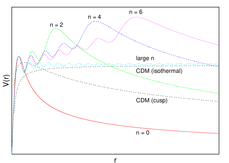
As can be seen on Fig. 1, the curve associated to the cold dark matter isothermal distribution (53) becomes flat at large distances as in the large $n$ case. It does not exhibit however the peak which all the other curves feature. At the outskirts of the system, the cuspy distribution (54) leads to a decrease of the rotation velocity with ${\cal V}^{2}\propto\log(r)/r$ while, in the $n=0,2,4,6$ states, the decrease is typically Keplerian. Near the origin, the scalar field configurations yield a core with constant density as in the isothermal case. This is in agreement with recent measurements of the rotation curves of low surface brightness spirals. Note the small wiggles of the excited configurations. This could provide an explanation for some peculiar rotation curves with oscillatory behavior – as proposed by [11] who obtains similar curves in his massless model. However we will not consider this possibility in this paper, since we focus in a first stage on universal rotation curves of spiral galaxies [13].

At this point, we must say a few words about the stability of such self–interacting bosons. Beside the Newtonian limit, a first complication arises from the fact that – for a given number $N$ of particles and number $n$ of nodes – there are actually several values of the mass $M$ corresponding to static, bounded and spherically symmetric configurations. Only the lowest energy state is stable. This phenomenon occurs above a critical particle number $N\sim 0.3\,({\rm M}_{\rm P}/m)^{2}$. In the Newtonian regime, we are much below this scale and, for a given set ($N,n$), there is a unique static configuration. A stronger condition is that the gravitating boson system should be stable against fission into free particles so that $M<Nm$. It was shown in [16] that this criteria is fulfilled by all states in the Newtonian limit, even for large values of $n$. In that regime, $M$ tends towards $N\,m$ when $n\rightarrow\infty$ at fixed $N$ (in Table I, the precision on $\bar{M}$ and $\bar{N}$ is not sufficient to see this effect). Stability against fission is only a necessary condition. More generally, one should check stability (i) at the classical level under any small perturbation leaving $N$ unchanged and (ii) at the quantum level under tunneling from excited states to the fundamental state. The former analysis was performed analytically by [17] who concludes on the stability of all excited states – at least in the Newtonian limit. A non–perturbative analysis was performed numerically in [21] and yielded the opposite conclusion. However, as clearly stated in [21], these simulations were based on the most general perturbations which were in particular allowed to violate the conservation of the particle number $N$. Therefore, the positive result of [17] seems to apply to our situation. As far as the stability under tunneling is concerned, we are not aware of any previous result. Notice anyway that, in order to be conservative, we will only consider $n=0$ fundamental state configurations in what follows.

IV Comparison with observations.

In general, reproducing the observed galactic rotation curves amounts in modeling the contribution of many components apart from the halo and the observed luminous disk, like a HI gas, a rotating bar or bulge, etc. In order to make a strong statement, we will restrict our analysis to the simplest case of spiral galaxies and on distances smaller than the optical radius $r_{\rm opt}$ defined as the radius of the sphere encompassing 83% of the luminous matter. Indeed, for spiral galaxies and on such distances, the only significant contributions to the total density arise from a stellar disk with exponential density profile, plus the unknown dark halo contribution: one can avoid introducing a plethora of free parameters describing the other components. On the basis of such considerations, Persic, Salucci and Stel [13] – hereafter denoted PSS – performed a detailed statistical study over about 1100 optical and radio rotation curves. They rescaled each rotation curve to the same size and amplitude by expressing the radius as $r/r_{\rm opt}$ and the speed as ${\cal V}(r)/{\cal V}(r_{\rm opt})$. The rescaled curves were found to depend only on a single parameter, the luminosity $M_{I}$. Galaxies were divided in eleven classes depending on their brightness $M_{I}$ and the authors provided for each group of spirals the average rotation curve in the range $r<1.1\,r_{\rm opt}$. They showed that for non–luminous galaxies, rotation curves are increasing near the optical radius while for brighter objects, they tend to become flat or they even slightly decrease. This result is remarkable insofar as the dynamical contribution of the luminous disk – known up to a constant bias factor $\beta$ – is slightly decreasing at $r_{\rm opt}$. The immediate conclusion is that faint galaxies are always dominated by their halo whereas bright spirals only need a very small contribution from non–luminous matter. This amazing one-to-one correspondance between the disk and halo core density, depending only on one parameter (the magnitude), is generally called the disk-halo conspiracy.

The purpose of this article is to investigate whether or not a non–interacting massive scalar field halo may account for the universal rotation curves of PSS. To achieve this goal, we must solve once again the Einstein and Klein–Gordon equations, adding to the former the contribution from the luminous disk. In order to keep a sherically symmetric metric, we will describe the gravitational impact of the disk as if it was spherical. This approximation is reasonable provided that the corresponding contribution to the mass budget of the system remains small – which is the case for faint spirals. In the opposite case, a much more complicated metric needs to be introduced in order to describe the aspherical distribution of luminous matter. We therefore add to the time–time Einstein equation the disk density contribution $\rho$. Should the disk be alone, the rotation curve would be [13]

$${\cal V}^{2}_{\rm disk}(r)\;=\;{\cal V}^{2}_{\rm disk}(r_{\rm opt})\;{\displaystyle\frac{1.97\,(r/r_{\rm opt})^{1.22}}{\left\{(r/r_{\rm opt})^{2}+0.78^{2}\right\}^{1.43}}}\;\;.$$ (55)

The density $\rho$ is easily derived from a simple Newtonian calculation

$$4\,\pi\,G\,\rho\,=\,{\displaystyle\frac{{\cal V}^{2}_{\rm disk}}{r^{2}}}\,+\,2\,{\displaystyle\frac{{\cal V}_{\rm disk}{\cal V}_{\rm disk}^{\prime}}{r}}\,=\,{\cal V}_{\rm disk}^{2}(r_{\rm opt})\;{\displaystyle\frac{f(r/r_{\rm opt})}{r_{\rm opt}^{2}}}\;\;,$$ (56)

where we introduce the dimensionless function

$$f(u)\equiv{\displaystyle\frac{4.38\;u^{-0.78}}{\left\{u^{2}+0.78^{2}\right\}^{1.43}}}\,-\,{\displaystyle\frac{5.64\;u^{1.22}}{\left\{u^{2}+0.78^{2}\right\}^{2.43}}}\;\;.$$ (57)

Note that this profile is only valid in the range $0.04\,r_{\rm opt}<r<2\,r_{\rm opt}$ since relation (55) obtains from the fit of a more complicated expression involving modified Bessel functions. Below $r<0.04\,r_{\rm opt}$, we maintain a constant density which would otherwise diverge. We have actually checked that the details of the disk mass density near the center do not affect our results.

Introducing the additional mass distribution $\rho$ of the luminous disk into the pure scalar case discussed in section III simply amounts to modify the time–time Einstein relation (25) into

$$2v^{\prime\prime}\,+\,v^{\prime 2}\,+\,\frac{4v^{\prime}}{\bar{r}}\;=\;-2\,e^{\displaystyle 2v}\,\left\{\left(1\,+\,e^{\displaystyle-2\bar{u}}\right)\,\bar{\sigma}^{2}\;+\;e^{-\displaystyle 2v}\,\bar{\sigma}^{{}^{\prime}2}\;+\;\bar{\rho}\right\}\;\;,$$ (58)

where the dimensionless disk density $\bar{\rho}$ may be expressed as

$$\bar{\rho}\;=\;{\displaystyle\frac{4\,\pi\,G}{m^{2}}}\,\rho\;\;.$$ (59)

The radius $\bar{r}$ and the scalar field $\bar{\sigma}$ have been previously defined in relation (38). The other Einstein equation (26) as well as the Klein–Gordon relation (24) are not affected. It is worth studying the limit of these equations in the Newtonian regime in order to gain intuition on their scaling behavior. As before, the relation $u=-v\simeq\bar{u}$ applies in this regime and the system reduces to

$$\bar{u}^{\prime\prime}\,+\,\frac{2}{\bar{r}}\,\bar{u}^{\prime} = 2\,\bar{\sigma}^{2}\;+\;\bar{\rho}\;\;,$$ (60)

$$\bar{\sigma}^{\prime\prime}\,+\,\frac{2}{\bar{r}}\,\bar{\sigma}^{\prime} = 2\,\bar{u}\,\bar{\sigma}\;\;.$$ (61)

Relation (42) is not modified whereas the disk mass density $\bar{\rho}$ is introduced in the right hand side term of expression (41) to yield Eq. (60). As before, the scale invariance of the solution becomes more obvious when these relations are expressed in terms of the quantities $S=\bar{\sigma}(r)/\bar{\sigma}(0)$ and $\bar{u}_{\rm red}=\bar{u}(r)/\bar{\sigma}(0)$. The system (60) and (61) becomes

$$\bar{u}_{\rm red}^{\prime\prime}\,+\,{\displaystyle\frac{2}{x}}\,\bar{u}_{\rm red}^{\prime}=2\,S^{2}\;+\;{\cal R}\;\;,$$ (62)

$$S^{\prime\prime}\,+\,{\displaystyle\frac{2}{x}}\,S^{\prime}=2\,\bar{u}_{\rm red}\,S\;\;.$$ (63)

The disk density enters through the dimensionless parameter

$${\cal R}\;=\;{\displaystyle\frac{\bar{\rho}}{\bar{\sigma}^{2}(0)}}\equiv{\displaystyle\frac{4\,\pi\,G}{m^{2}}}\,{\displaystyle\frac{\rho}{\bar{\sigma}^{2}(0)}}\;\;.$$ (64)

Should ${\cal R}$ vanish, the fundamental $n=0$ mode solution for $S(x)$ would be uniquely determined. Taking advantage of relations (56) and (57) allows to express the disk contribution ${\cal R}$ as

$${\cal R}\;=\;{\displaystyle\frac{{\cal V}^{2}_{\rm disk}(r_{\rm opt})}{\bar{\sigma}(0)}}\;\left\{x_{\rm opt}^{-2}\;f\left({\displaystyle\frac{x}{x_{\rm opt}}}\right)\right\}\;\;.$$ (65)

The general scale–invariant solution $S(x)$ in the presence of a disk depends now on the parameters

$$\alpha\equiv x_{\rm opt}\,=\,m\,r_{\rm opt}\,\sqrt{\bar{\sigma}(0)}\quad{\rm and}\quad\gamma\,=\,{\displaystyle\frac{{\cal V}^{2}_{\rm disk}(r_{\rm opt})}{\bar{\sigma}(0)}}\;\;,$$ (66)

which come into play through the disk density

$${\cal R}\left\{\alpha,\gamma\right\}\;=\;\gamma\,\alpha^{-2}\,f\left(x/\alpha\right)\;\;.$$ (67)

The radial extension $x_{\rm opt}$ of the matter disk relative to the scalar halo is accounted for by the parameter $\alpha$. Since the scalar field generates a rotation curve whose magnitude ${\cal V}^{2}$ scales as $\bar{\sigma}(0)$, the quantity $\gamma$ measures the dynamical impact of the disk relative to that of the halo. These parameters determine therefore the size and the mass of the disk with respect to the halo in which it is embedded. The actual scale of the entire system is specified in turns by – say – the optical radius $r_{\rm opt}$ and the disk speed ${\cal V}_{\rm disk}(r_{\rm opt})$. Once the configuration $\left\{\alpha,\gamma\right\}$ is chosen, the behavior of the field – given by the scale–invariant solution $S_{\alpha\gamma}(x)$ to the system (62) and (63) – is completely determined. The full rotation curve which both disk and halo generate may be readily derived.

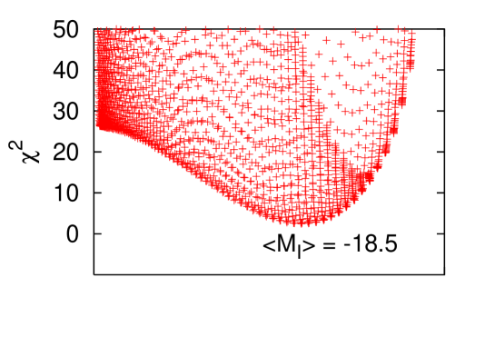
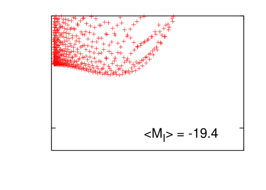
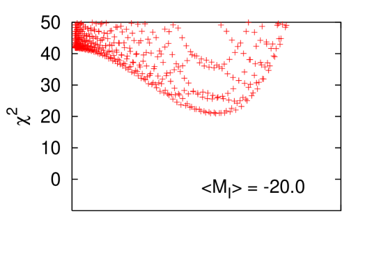
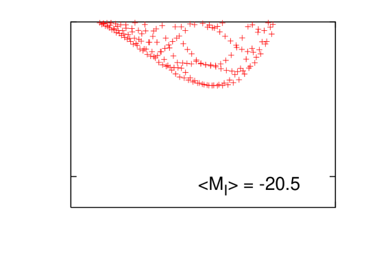
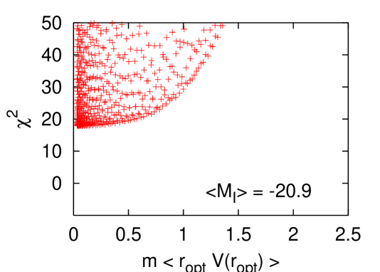
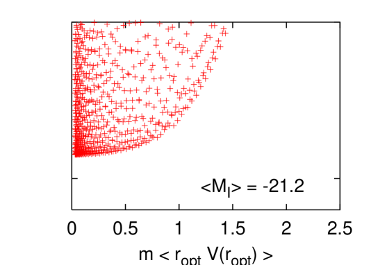
With a $\chi^{2}$ analysis, we obtain likelihood contours in the two–dimensional free parameter space $\{\alpha,\gamma\}$ shown on Fig. 2.

FIG. 2.: Two–dimensional likelihood contours in the $\{\alpha,\gamma\}$ space, for six galaxy classes ordered by growing magnitude. In the four first cases, the crosses show the best–fit models. For the last two cases, the minimum is strongly degenerate along a line ranging from $\alpha=0$ to $\alpha=0.5$. The curves correspond to $\chi^{2}-\chi^{2}_{\rm min}=3.2$ (resp. $6.2$), which would give the 68% (resp. 95%) allowed region if the experimental errors could be rigorously interpreted as 1–$\sigma$ gaussian errors.

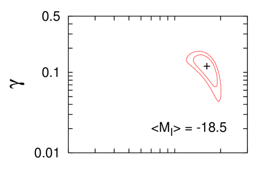
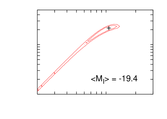
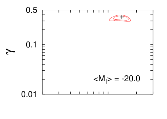
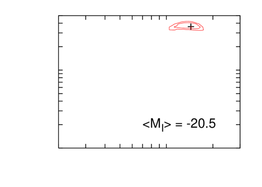
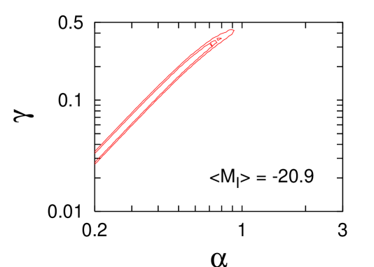
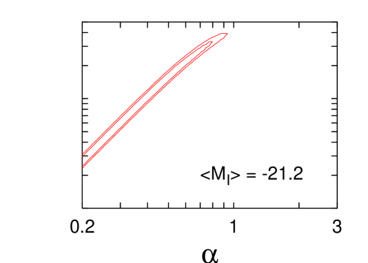
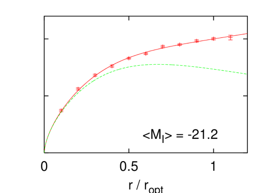
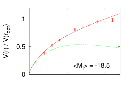
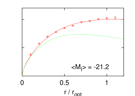
We use only the six less luminous galaxy classes from PSS since they are the most relevant probes of the halo contribution and a priori the closest cases to spherical symmetry – brighter galaxies require only a small halo contribution, at least inside the optical radius. The minimum $\chi^{2}$ values are (2.5, 23.6, 20.9, 29.4, 17.8,7.6), and the corresponding best–fit rotation curves are shown on Fig. 3.

FIG. 3.: In each panel, the theoretical rotation curve corresponds to the $\left\{\alpha,\gamma\right\}$ configuration that provides the best fit to the data. The dashed lines shows the contribution of the disk, which increases with the galaxy magnitude as for usual CDM models.

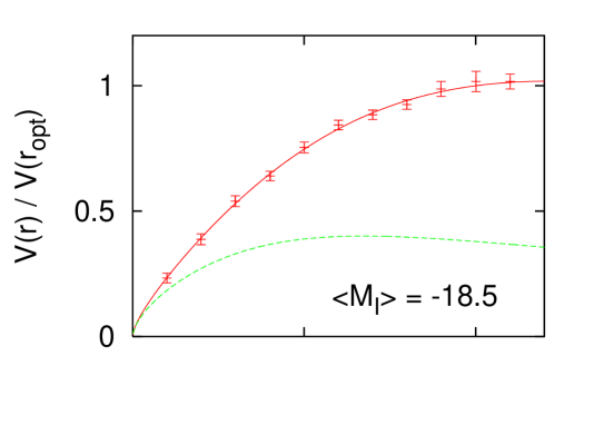
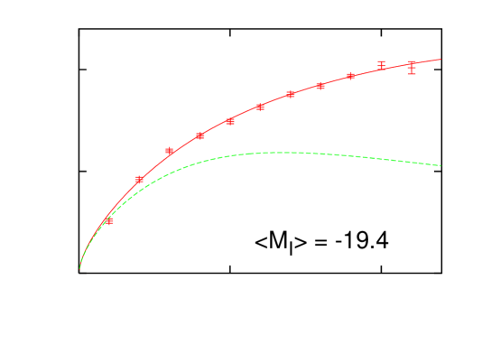
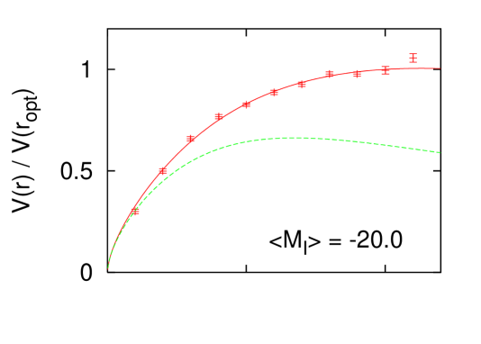
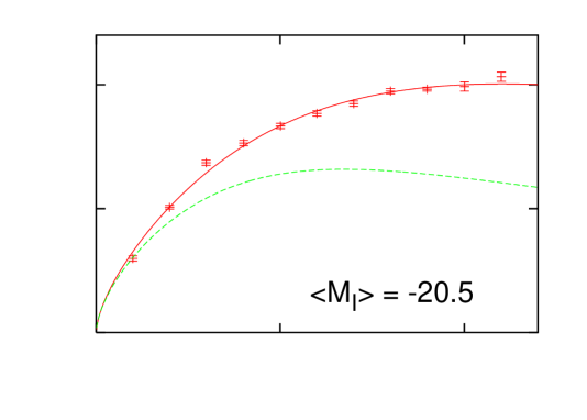
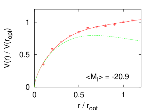
We will not over–interpret the absolute value of the $\chi^{2}$ in terms of goodness–of–fit, because we do not know the exact meaning of the data error bars. A careful examination shows that the points are not distributed according to their very small errors, at least if the data are to be explained by smooth curves – this is visible for instance with the third point in the $<M_{I}>=-20.5$ case, which explains why the minimal $\chi^{2}$ is only 29.4. Therefore, there is a hint either that the errors are slightly underestimated, or that the data feature small wiggles corresponding e.g. to spiral arms, that should enter into a better modelization of the disk density. Anyway, even with the given error bars, the $\chi^{2}$ are already fairly good and our scalar halo model seems to fit universal rotation curves at least as well as the toy–model CDM halo used by PSS. We also note that for the last two cases, the minimum is strongly degenerate along a line ranging from $\alpha=0$ to $\alpha=0.5$. So, for the most luminous galaxies, the data provide only a lower bound on the halo size, while for the other cases a specific value is preferred.

FIG. 4.: The constellation of $\left\{\alpha,\gamma\right\}$ configurations is featured in the plane $(m\left<r_{\rm opt}{\cal V}_{\rm opt}\right>,\chi^{2})$. Faint galaxies have a preferred mass while the brighter ones in the two last panels provide only an upper bound.

FIG. 5.: In each panel, the average value $\left<r_{\rm opt}{\cal V}_{\rm opt}\right>$ over the corresponding spiral galaxies has been used to get the scalar field mass $m\,=\,\alpha\sqrt{\gamma}/(r_{\rm opt}\,{\cal V}_{\rm opt})$. The best fit configurations with a common value of the mass $m=6\times 10^{-24}\,{\rm eV}$ are shown in solid lines, together with the observations. Again, the dashed line shows the contribution from the disk only.

For each individual galaxy, one can restore the physical value of the rotation velocity by adjusting the free scaling parameter $\bar{\sigma}(0)$. The mass of the scalar field is given by

$$m^{2}\,=\,{\displaystyle\frac{\alpha^{2}\,\gamma}{r_{\rm opt}^{2}\;\beta\;{\cal V}^{2}(r_{\rm opt})}}\;\;.$$ (68)

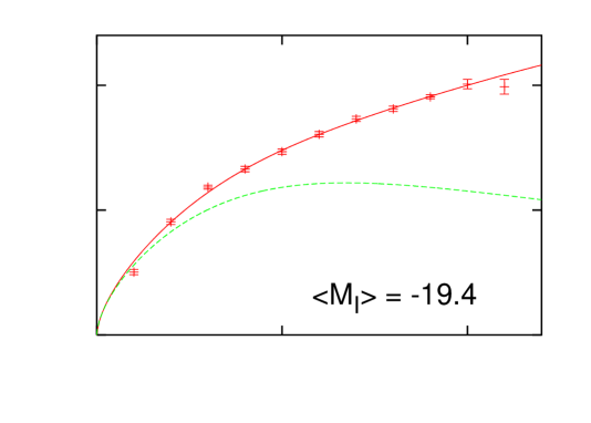
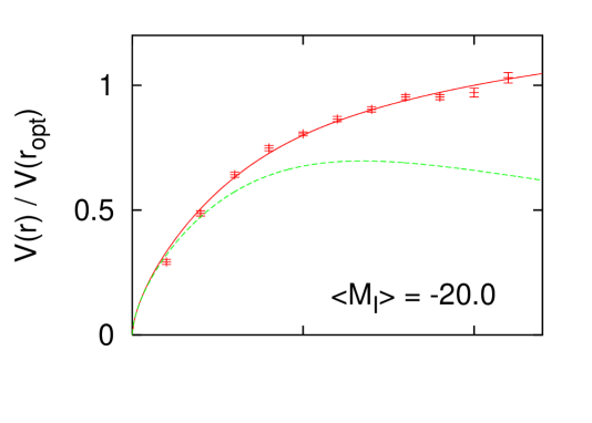
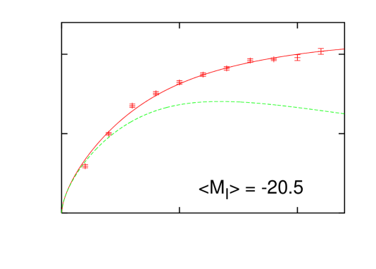
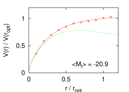
Here we defined the parameter $\beta={\cal V}_{\rm disk}^{2}(r_{\rm opt})/{\cal V}^{2}(r_{\rm opt})$, calculated by the code for each value of the relevant parameters $\{\alpha,\gamma\}$. Of course, our model can provide a powerful explanation for galactic rotation curves only if all galaxies can be fitted simultaneously with the same value of $m$, and therefore approximately the same angular velocity $\omega$ (in principle one could introduce a time-dependant effective mass, with slightly different values at large and small redshifts; however, since galaxy rotation curves have never been found to be redshift-dependant, we discard this possibility and assume that $m$ is constant in space and time, at least on observable scales). In order to test this idea, it would be natural to use data from individual galaxies; but in doing so, one would face back the problems associated with large systematic uncertainties, which motivate the PSS approach. In a first step, we plot $\chi^{2}$ as a function of $m\;r_{\rm opt}\,{\cal V}(r_{\rm opt})$ in Fig. 4 and remark that the faint galaxies have a preferred mass while the brighter ones in the two last panels provide only an upper bound. Then, we assume that each synthetic universal rotation curve is associated with a unique typical galaxy, with average optical radius and velocity. For each class of magnitude, we perform an average on the sub–sample given by PSS – see the tables in their Appendix D – and find respectively $\left<r_{\rm opt}{\cal V}(r_{\rm opt}\right>=710$, 1100, 1900, 2500, 3200 and 4900 kpc km s^-1. Since we do not employ the raw 600 galaxy data, we cannot give an error on these numbers, nor can we make a precise prediction for the mass. However, plotting now the $\chi^{2}$ as a function of $m$, we find that the first four classes are perfectly compatible with a mass $m\in[4-16]\times 10^{-24}\,{\rm eV}$ while the two others push towards the lower–end of this interval with $m\in[4-8]\times 10^{-24}\,{\rm eV}$. On Fig. 5, we plot the rotation curves obtained with $m=6\times 10^{-24}\,{\rm eV}\simeq 5\times 10^{-52}$ M_P and minimized over $\gamma$. Although the $\chi^{2}$ values are approximately 1.5 bigger than those of the independent best–fits of Fig. 3, the agreement with the data remains quite good. The effect of fixing the mass is to obtain more radical behaviors at $r_{\rm opt}$: for light galaxies, the rotation curves are growing faster near the optical radius while for bright galaxies they are even flatter. For all these models, the total mass is close to $M=5\times 10^{10}\,{\rm M_{\odot}}$ whereas the ratio of the total radius over the optical radius – which respectively encompass 83% of the total and luminous mass – varies between 4 for $<M_{I}>=-18.5$ and 1.5 for $<M_{I}>=-21.2$.

V Discussion and prospects.

In this work, we solved the Einstein and Klein–Gordon equations for a free massive scalar field, in presence of a baryonic disk. Using the universal curves of Persic, Salucci and Stel [13], which are based on hundreds of galaxies, we showed that a galactic halo consisting in such a Bose condensate could explain fairly well the rotation of low–luminosity spiral galaxies. A single value of the mass, of order $6\times 10^{-24}$eV, is compatible with galaxies of different magnitudes. The corresponding Compton wavelength $1/m\simeq 10^{-2}$ kpc is three orders of magnitudes smaller than the typical size of spirals. Indeed, the spatial extension of a self–gravitating field $\Phi$ is given approximately by $1/(\sqrt{\Phi(0)}~{}m)$, while the square root of the central field value (expressed in Planck units) is comparable with the velocity of orbiting particles (in units of $c$). Since we are dealing with speeds ${\cal V}\sim 100$ km s${}^{-1}~{}\sim 10^{-3}\,c$, there is really a factor of $10^{3}$ between the Compton wavelength and the size of the halo. Note that since $\omega\simeq m$, the light scalar field $\Phi$ rotates in its internal space with a period of $\sim 30$ yr.

We conclude that scalar fields could be a nice alternative to CDM halo models. Our positive results concerning the rotation curves are strengthened by other astrophysical considerations. First, a scalar field solves naturally the dynamical friction issue for bared galaxies. Because it is completely smooth, such an extended field cannot slow down the spinning bars observed at the centers of many galaxies, as would a granular CDM medium. Second, following Hu, Barkana and Gruzinov [22], an ultra–light scalar field can avoid the excess of small–scale structure predicted by CDM simulations near the galactic center.

Of course, several improvements are needed before concluding that a scalar field is the best galactic dark matter candidate on the market. First, it is necessary to extend the comparison to various types of individual galaxy rotation curves, with the drawback that more degrees of freedom must be included in realistic modelizations of the baryonic components (gas, bulge, …). This is however the only way to obtain better constraints on $m$, and to find out whether a quartic coupling, not considered in this analysis, improves the model. In some particular cases, it would be worth taking into account excited field configurations, which seem to be stable (due to charge conservation) and which predict ultra–flat rotation curves far from the core, with small wiggles that may have already been observed (see also the claim in [23] concerning possible existence of discrete dynamical classes for spiral galaxy disks). Also, in order to get a better view of the rotation curves in the vicinity of the core, especially for bright spiral galaxies, further technical ingredients must be passed to the equations, in order to distinguish the spherical symmetry of the halo from the quasi two–dimensional distribution of the stars.

Finally, it would be extremely interesting to plug such a complex light scalar field into a general cosmological framework, and study into details the growth of linear perturbations and the formation of non–linear structures. The pioneering discussions on such cosmological scenarios [22, 24] are very promising and suggest that many interesting developments on scalar field dark matter should arise in the next years.

REFERENCES

- [1] A. T. Lee et al., astro-ph/0104459; C. B. Netterfield et al., astro-ph/0104460; N. W. Halverson et al., astro-ph/0104489; C. Pryke, N. W. Halverson, E. M. Leitch, J. Kovac, J. E. Carlstrom, W. L. Holzapfel and M. Dragovan, astro-ph/0104490.
- [2] S. Perlmutter et al. [Supernova Cosmology Project Collaboration], Astrophys. J. 517, 565 (1999).
- [3] R. R. Caldwell, R. Dave and P. J. Steinhardt, Phys. Rev. Lett. 80, 1582 (1998); E. J. Copeland, A. R. Liddle and D. Wands, Phys. Rev. D 57, 4686 (1998); A. R. Liddle and R. J. Scherrer, Phys. Rev. D 59, 023509 (1999); P. J. Peebles and A. Vilenkin, Phys. Rev. D 59, 063505 (1999); P. Binétruy, Phys. Rev. D 60, 063502 (1999); P. J. Steinhardt, L. Wang and I. Zlatev, Phys. Rev. D 59, 123504 (1999); P. Brax and J. Martin, Phys. Lett. B 468, 40 (1999); A. Riazuelo and J. Uzan, Phys. Rev. D 62, 083506 (2000); T. Matos, F. S. Guzman and L. A. Urena-Lopez, Class. Quant. Grav. 17, 1707 (2000); T. Matos and L. A. Urena-Lopez, Phys. Rev. D 63, 063506 (2001).
- [4] S. Burles and D. Tytler, Astrophys. J. 499, 699 (1998); Astrophys. J. 507, 732 (1998).
- [5] B. Moore et al., Astrophys. J. 524, L19 (1999).
- [6] W. B. Lin, D. H. Huang, X. Zhang and R. Brandenberger, Phys. Rev. Lett. 86, 954 (2001).
- [7] D. N. Spergel and P. J. Steinhardt, Phys. Rev. Lett. 84, 3760 (2000).
- [8] J. Goodman, astro-ph/0003018.
- [9] A. Riotto and I. Tkachev, Phys. Lett. B 484, 177 (2000).
- [10] T. Matos, F. S. Guzman and D. Nunez, Phys. Rev. D 62, 061301 (2000); T. Matos and F. S. Guzman, Class. Quant. Grav. 17, L9 (2000); F. S. Guzman, T. Matos and H. Villegas-Brena, Rev. Mex. A. & A. 37, 63 (2001); T. Matos, F. S. Guzman, L. A. Urena-Lopez and D. Nunez, astro-ph/0102419.
- [11] F. E. Schunck, astro-ph/9802258.
- [12] U. Nucamendi, M. Salgado and D. Sudarsky, Phys. Rev. D 63, 125016 (2001).
- [13] M. Persic, P. Salucci and F. Stel, Mon. Not. Roy. Astron. Soc. 281, 27 (1986).
- [14] V. Sahni and L. Wang, Phys. Rev. D 62, 103517 (2000).
- [15] R. Ruffini and S. Bonazzola, Phys. Rev. 187, 1767 (1969).
- [16] R. Friedberg, T. D. Lee and Y. Pang, Phys. Rev. D 35, 3640 (1987).
- [17] P. Jetzer, Phys. Rept. 220, 163 (1992).
- [18] A. R. Liddle and M. S. Madsen, Int. J. Mod. Phys. D 1, 101 (1992).
- [19] S. Weinberg, Gravitation and Cosmology (Wiley, New York, 1972).
- [20] J. F. Navarro, C. S. Frenk and S. D. M. White, Astrophys. J. 462, 563 (1996).
- [21] J. Balakrishna, E. Seidel and W. Suen, Phys. Rev. D 58, 104004 (1998).
- [22] W. Hu, R. Barkana and A. Gruzinov, Phys. Rev. Lett. 85, 1158 (2000).
- [23] D. F. Roscoe, astro-ph/0107300, to appear in MNRAS
- [24] L. A. Boyle, R. R. Caldwell and M. Kamionkowski, astro-ph/0105318