The H i supershell GS061+00+51 and its neighbours

We describe H i observations of a $4{\degr}\times 4{\degr}$ field in the Milky Way centered on $l=61{\degr}$, $b=0{\degr}$ made by the Effelsberg radiotelescope. The field contains one previously identified H i supershell, GS061+00+51 (Heiles, 1979); apart from it we find several new structures. We also study the H i distribution in the vicinity of four H ii regions, S86, S87, S88 and S89. We confirm the existence of the shell GS061+00+51, and we find that it has two smaller neighbours, spherical shells with $R_{\mathrm{sh}}\sim 30\ \mathrm{pc}$. We identify at least one more regular shell at $v_{\mathrm{LSR}}=-18\ \mathrm{kms^{-1}}$; and one blown-out shell at $v_{\mathrm{LSR}}=-54\ \mathrm{kms^{-1}}$. In two cases we are able to connect H ii regions with features in the H i distribution (S86 and S87), in two other cases no connection is found. Apart from quite regular H i shells we see a number of non-coherent objects, which are probably a result of the turbulence in the interstellar medium.

1 Introduction

Turbulence creates in the interstellar medium (ISM) many structures, typically dense sheets, clumps and low-density holes. The majority of these structures are transient. Many of them have an irregular, patchy appearance; however, some may look like ordinary, regular objects.

Another type of structures found in the ISM are H i shells and holes. We agree with Walter & Brinks (1999), that there is a difference between turbulent structures and H i shells, at least in the sense that most turbulent structures show very little consistency if any in the position-velocity (or position-position) space, while H i shells do. This, of course, does not mean, that the turbulent medium does not influence the shape and evolution of H i shells. It does, and as a first guess we may estimate that shapes of shells in a turbulent medium will be more irregular than in a smooth medium.

We observed a field in the galactic plane, which contains the supershell GS061+00+51 (Heiles, 1979). Our observations have four times higher resolution than the survey of Weaver & Williams (1973) used for the previous identification. Apart from the shell GS061+00+51 and its surroundings we study the rest of the datacube and try to identify new shells and shell-like structures.

In the observed field four optical H ii regions are known (S86, S87, S88 and S89; Sharpless, 1959), at least one of them (S86) is connected to an OB association (Vul OB1). The angular dimensions of the mentioned H ii regions are greater than or comparable to the resolution of our observations, and therefore we should be able to see their imprint in the H i distribution.

2 Observations, data reduction

In 1997 (March–June) we observed a $4{\degr}\times 4{\degr}$ field in the Milky Way centered on $l=61{\degr}$, $b=0{\degr}$ with the 100 m radiotelescope in Effelsberg at the frequency 1.4 GHz (21 cm) of the neutral hydrogen line. The frequency switching mode was used. The bandwidth 1.56 MHz was split into 512 channels with the width of $\sim$3 kHz, or 0.64 $\mathrm{kms}^{-1}$. The primary beamwidth of the Effelsberg radiotelescope at 21 cm is 9.4 arcmin, observations were made with a spacing of 4 arcmin (the pixel size). Each spectrum was integrated for 15 s. The data were calibrated using the standard S7 procedure (Kalberla et al., 1982) and a linear baseline was subtracted. Observations were made in 6 runs, each dataset was calibrated separately. Data were not corrected for stray radiation, because we observed a small field and were mostly interested in the differential effect of the observed emission against the background. Radio frequency interference may be present in the observational data.

To check our observations we compared them with data from the Leiden-Dwingeloo H i survey (Hartmann & Burton, 1997), which had a resolution of $0.5{\degr}$. To match the Dwingeloo beam we averaged spectra from 81 pixels, i.e. (36 arcmin)². A comparison between our data and the Dwingeloo survey is shown in Fig. 1, where good agreement between the two datasets is visible.

Figure 1: A comparison between the Leiden-Dwingeloo survey (thick line) and our observations (thin line). Our spectra are artificially offset by 10 K.

3 Identification of H i shells

To be ranked among H i shells, a structure must fulfill several criteria:

• it is either a hole – i.e. a region of lower brightness temperature, or a shell – a sheet of higher temperature, or both – a hole encircled by a shell;

• it must be visible in several consecutive velocity channels, gradually changing its size;

• preferably, it should be expanding.

The identification was made by eyes and this process is quite subjective. Both the eye and the criteria stated above have a bias towards regular (spherical) and compact structures, while less regular structures are overlooked; the type of background (smooth vs. turbulent) also plays an important role. We suppose that the identified structures are real, but we definitely missed some shells, especially in crowded or very turbulent regions.

Due to the size of the field, many structures are only partly visible, and those we do not describe here (of the known H i shells GS064-0.1-97 (Heiles 1979) is seen in channel maps as a partial arc). Another previously known structure, the shell GS061+00+51, lies fully in the observed field.

Figure 2: $\Delta T_{\mathrm{B}}$ graph of the shell GS59.9-1.0+38. The left panel shows the spectrum through the center of the shell (solid line) and the average spectrum of the surrounding area (dotted line). The right panel shows their difference $\Delta T_{\mathrm{B}}$, where both walls (receding and approaching) belonging to the structure and the hole (corresponding to the swept-up region) are nicely recognizable.

3.1 $\Delta T_{B}$ graphs

The spectrum of an H i shell (in an ideal case) contains two peaks corresponding to the intersection of the line of sight with dense walls and a depression corresponding to the hole. These features are superimposed on the spectrum emitted by the surrounding ISM. To disentangle the two contributions, we subtract the background emission from the spectrum through the structure; the shell features should then appear. The column densities of the gas swept up into the wall can be — under some assumptions on the shape and dimensions of the shell — transformed into the mass of the shell and the initial volume density of the ISM.

However, to determine the background spectrum is difficult, first because of the unknowns in the velocity field and gas distribution which shape the spectrum, secondly because of the turbulent character of the ISM. The simplest way to define the background is to take the average of the emission from a region around the studied line of sight (in the case of studying the spectrum through the H i shell the region should contain the whole structure). This approach has its drawbacks, but at least it smears out the small scale inhomogeneities. When applied to artificial datacubes, we find, that often this method leads to a slight underestimation of the real values (lower column densities of the swept-up gas and lower masses).

An important “spoiler” is the non-zero velocity dispersion of the gas, both in the shell and in the ISM. How important this effect is, depends on the ratio between the velocity dispersion and the expansion velocity. The line widths of the walls correspond to the real velocity dispersion in the gas swept in the shell. The line width of the hole is not so easy to classify and so we abstain from any deductions.

It is also possible to estimate masses purely from the dimensions of the shell and an assumed (or estimated or fitted) density $n_{0}$ of the ISM. This approach, due to the variability of $n_{0}$ on many scales, does not lead to better or more reliable results.

3.2 Distances and energetics

To calculate kinematic distances of shells we use the rotation curve of Wouterloot et al. (1990).

The total energy $E_{\mathrm{tot}}$ required to create the H i shell is estimated using the Chevalier (1974) formula

$${E_{\mathrm{tot}}\over\mathrm{erg}}=5.3\times 10^{43}\left({n_{0}\over\mathrm{cm}^{-3}}\right)^{1.12}\left({R_{\mathrm{sh}}\over\mathrm{pc}}\right)^{3.12}\left({v_{\mathrm{exp}}\over\mathrm{kms}^{-1}}\right)^{1.4}$$ (1)

where $n_{0}$ is the density of the ambient medium, $R_{\mathrm{sh}}$ the radius of the shell and $v_{\mathrm{exp}}$ its expansion velocity.

4 H i shells: description

4.1 GS59.9-1.0+38

	FWHM	$N_{\mathrm{{H\textsc{i}}\leavevmode\nobreak\ }}$	$m_{\mathrm{{H\textsc{i}}\leavevmode\nobreak\ }}$
	($\mathrm{kms^{-1}}$)	($\mathrm{cm^{-2}}$)	($M_{\sun}$)
hole	7.1	$1.5\times 10^{20}$	$2.9\times 10^{3}$
wall 1	3.2	$4.6\times 10^{19}$	$5.6\times 10^{3}$
wall 2	2.6	$3.7\times 10^{19}$	$4.5\times 10^{3}$

Table 1: GS59.9-1.0+38: FWHM is the width of the line, $\mathrm{N_{{H\textsc{i}}\leavevmode\nobreak\ }}$ is the column density of H i swept up into the wall or missing in the hole derived from the spectrum through the centre of the shell, $m_{\mathrm{{H\textsc{i}}\leavevmode\nobreak\ }}$ is the mass of H i swept up in walls or missing in the hole, assuming the radius of 35 pc.

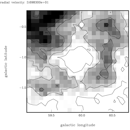
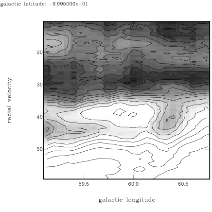
Figure 3: The shell GS59.9-1.0+38 in a velocity channel ($v_{\mathrm{LSR}}=+37.0\ \mathrm{kms^{-1}}$) and the $lv$ cut ($b=-1.0^{\degr}$). The grey scale goes from white (the lowest temperature) to black (the highest temperature). The range of temperatures in the left panel is (22.9 K, 61.5 K), contour values are 26.8 (1.9) 57.7 K; in the right panel the range is (0.5 K, 88.8 K), contour values are 9.3 (4.4) 80.0 K.

GS59.9-1.0+38 is a small, probably young, spherical structure (see Fig. 3). Both the approaching and receding hemisphere and a change of the shell diameter as a function of the radial velocity are seen. The shell is located in the inner Galaxy at the terminal velocity. Its dimensions are $60\times 52$ arcmin, corresponding to a radius of roughly 35 pc; its expansion velocity is 9 $\mathrm{kms}^{-1}$. The right panel of Fig. 3 may indicate a lower expansion velocity: a large gradient of the brightness temperature with the velocity in this area hides a part of the approaching hemisphere of the shell. Individual channel maps or the $\Delta T_{\mathrm{B}}$ graph — see Fig. 2 or Ehlerová (2000) — show the higher expansion velocity.

Quantities derived from the $\Delta T_{B}$ graph (see Fig. 2) are summarized in Table 1. FWHM gives the width of the line (if the line profile is Gaussian, the dispersion $\sigma\simeq 0.6\ \mathrm{FWHM}$); $\mathrm{N_{{H\textsc{i}}\leavevmode\nobreak\ }}$ is the column density of H i swept up into the wall (or missing in the hole); $m_{\mathrm{{H\textsc{i}}\leavevmode\nobreak\ }}$ is the derived mass of H i swept up in walls (or missing in the hole), assuming the radius of the shell to be 35 pc.

The velocity dispersion of the gas swept into the shell is quite small (1.5–2.0 $\mathrm{kms^{-1}}$) which is in agreement with the expected high cooling rate in dense walls.

The masses derived from walls and a hole are not the same, but this is not very surprising, given the method and uncertainties in deriving the background (see the section “$\Delta T_{B}$ graphs”). As a reasonable estimate we adopt the value of the total mass $m_{\mathrm{tot}}$ ($m_{\mathrm{tot}}=m_{{H\textsc{i}}\leavevmode\nobreak\ }/0.7$, where 0.7 is the solar abundance of hydrogen):

$$m_{\mathrm{tot}}=5.2\times 10^{3}M_{\sun}.$$

The corresponding volume density of the ISM at the position of the ISM before the creation of the shell is

$$n_{0}=0.9\ \mathrm{cm}^{-3}.$$

The energy needed to create the structure is (from Eq. 1):

$$E_{\mathrm{tot}}=0.7\times 10^{50}\mathrm{erg}.$$

This value is smaller than the ”canonical” energy of one supernova, $E_{\mathrm{SN}}=10^{51}\mathrm{erg}$. This, in fact, is not unusual for observed shells, see e.g. Heiles (1979).

The shell GS59.9-1.0+38 is probably young, from the analytical solution (Sedov, 1959) we estimate its expansion age as $\simeq 1.5$ Myr.

4.2 GS59.7-0.4+44

	FWHM	$N_{\mathrm{{H\textsc{i}}\leavevmode\nobreak\ }}$	$m_{\mathrm{{H\textsc{i}}\leavevmode\nobreak\ }}$
	($\mathrm{kms^{-1}}$)	($\mathrm{cm^{-2}}$)	($M_{\sun}$)
hole	8.4	$2.7\times 10^{20}$	$4.0\times 10^{3}$
wall	7.7	$1.2\times 10^{20}$	$1.0\times 10^{4}$

Table 2: GS59.7-0.4+44: FWHM is the width of the line, $\mathrm{N_{{H\textsc{i}}\leavevmode\nobreak\ }}$ is the column density of H i swept up into the wall or missing in the hole derived from the spectrum through the centre of the shell, $m_{\mathrm{{H\textsc{i}}\leavevmode\nobreak\ }}$ is the mass of H i swept up in walls or missing in the hole, assuming the radius of 30 pc. Only the receding wall is visible in velocity channels.

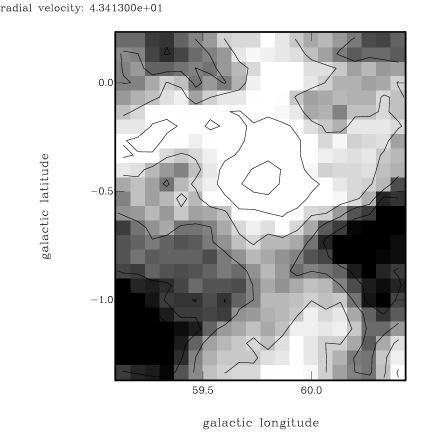
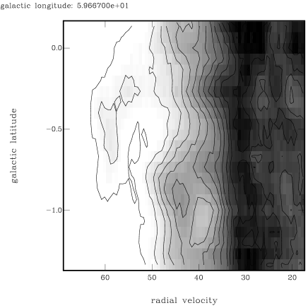
Figure 4: The shell GS59.7-0.4+44 in a velocity channel ($v_{\mathrm{LSR}}=+43.4\ \mathrm{kms^{-1}}$) and the $bv$ cut ($l=59.67^{\degr}$). The grey scale goes from white (the lowest temperature) to black (the highest temperature). The range of temperatures in the left panel is (4.5 K, 51.6 K), contour values are 9.2 (2.4) 46.8 K; in the right panel the range is (0.0 K, 91.3 K), contour values are 7.7 (4.6) 82.0 K.

GS59.7-0.4+44 (see Fig. 4) is another small spherical structure, in fact it is nearly a twin of GS59.9-1.0+38. Like GS59.9-1.0+38, GS59.7-0.4+44 lies close to the tangential point. Its radius is 24 arcmin (30 pc), its expansion velocity is 14 $\mathrm{kms}^{-1}$ (for the explanation of the seemingly lower expansion velocity in the $bv$ diagram see the previous section). Table 2 summarizes observed properties of the shell.

A reasonable mass estimate is

$$m_{\mathrm{tot}}=7.5\times 10^{3}M_{\sun}$$

corresponding to

$$n_{0}=2.1\ \mathrm{cm}^{-3}.$$

Chevalier’s estimate of the energy needed to create the shell GS59.7-0.4+44 is

$$E_{\mathrm{tot}}=2.0\times 10^{50}\mathrm{erg}.$$

As in the case of GS59.9-1.0+38 this energy is smaller than the canonical value, but we suppose that the shell could have been created by one supernova explosion.

The age of the shell is small, only about 1 Myr.

4.3 GS061+00+51

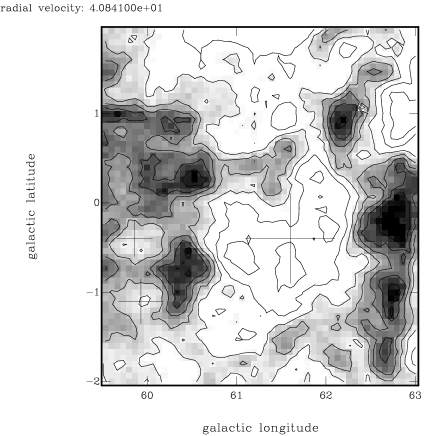
Figure 5: The shell GS061+00+51 in a velocity channel ($v_{\mathrm{LSR}}=+40.8\ \mathrm{kms^{-1}}$) and the $lv$ cut ($b=-0.53^{\degr}$). Three crosses in the left panel show centers of H i shells GS061+00+51, GS59.9-1.0+38 and GS59.7-0.4+44. The grey scale goes from white (the lowest temperature) to black (the highest temperature). The range of temperatures in the left panel is (7.0 K, 66.9 K), contour values are 13.0 (3.0) 61.0 K; in the right one panel the range is (0.0 K, 102.6 K), contour values are 8.7 (5.2) 92.2 K.

This is one of Heiles’ expanding shells (Heiles, 1979), the only complete shell in our field which was known before. Its first detection and description can be found in Katgert, 1969. A receding part of the shell is not visible. The approaching hemisphere is seen clearly, and is quite interesting. It is not a classical elliptical shell, but, especially at lower velocities, it resembles a crescent (see Fig. 5). We can think of two possibilities to explain this shape:

1. Merging theory:
   The shell was created by the merging of 3 (or more) small bubbles, each of them created by a stellar wind of one star or one supernova explosion. The bubbles interacted, but their untouched parts continued to expand, which led to a kind of ”circularization”. Apart from the shape this theory also explains the denser walls inside the hole (they are not seen very well in the printed version of the picture).

2. Cloud theory:
   An originally quite regular shell encountered during the expansion a high density cloud. The cloud distorted the shape of the shell; at the places, where the shell emerged from the cloud, the expansion tends to make it spherical. Alternatively, the explosion (which created the shell) took place off center in a high density cloud, with a subsequent asymmetrical expansion.

GS061+00+51 is found near the terminal velocity. Its dimensions are $\sim 2.4{\degr}$ in the $l$ direction and $2.9{\degr}$ in the $b$ direction, corresponding to 169 pc and 202 pc, respectively (depending on how you define the edge of the shell). Its expansion velocity is roughly 13 $\mathrm{kms}^{-1}$, only one hemisphere is seen, in $\Delta T_{\mathrm{B}}$ graphs no reliable walls are identified.

The properties of the shell are:

$N_{\mathrm{{H\textsc{i}}\leavevmode\nobreak\ }}=3.7\times 10^{20}\mathrm{cm^{-2}}$

$m_{\mathrm{tot}}=1.0\times 10^{5}M_{\sun}$

$n_{0}=1.0\ \mathrm{cm^{-3}}$

$E_{\mathrm{tot}}=2.6\times 10^{51}\mathrm{erg}$.

The energy, which created the shell, was probably released in one or more supernova explosions. The estimate of the shell age is $\tau\simeq 4$ Myr.

The dimensions of the structure as given by Heiles (1979) are slightly higher than our values, which is caused by 1) the fact, that the resolution of the Effelsberg radiotelescope is higher than that of the survey in which Heiles identified the shells: viz. the H i survey of Weaver & Williams (1973) with a spatial resolution of $36\ \mathrm{arcmin}$ and a velocity resolution of 2 $\mathrm{kms}^{-1}$; and 2) uncertainties in defining the precise boundaries of the shell — while there is no doubt about the existence and position of the structure, it is not completely clear, if all adjoining depressions belong to it.

Obviously (see Fig. 5), shells GS061+00+51, GS59.9-1.0+38 and GS59.7-0.4+44 are neighbours. GS061+00+51 is older and bigger than the other two, but not old enough to trigger secondary star formation in the walls, which could result in the creation of new small shells on the rim of the old structure. We may be witnessing propagating star formation in one cloud (or a cloud complex) which started at higher galactic longitudes and propagates toward the lower longitudes. The difference in ages of GS061+00+51, GS59.9-1.0+38 and GS59.7-0.4+44 is about 3-4 Myr, which suggests that the speed of the shock front compressing the gas and triggering the star formation is around 40 $\mathrm{kms}^{-1}$ (this is a lower limit since we do not take into account the differences in radial distances). In a few million years the three bubbles should merge.

4.4 GS62.1+0.2-18

	FWHM	$N_{\mathrm{{H\textsc{i}}\leavevmode\nobreak\ }}$	$m_{\mathrm{{H\textsc{i}}\leavevmode\nobreak\ }}$
	($\mathrm{kms^{-1}}$)	($\mathrm{cm^{-2}}$)	($M_{\sun}$)
hole	10.3	$3.7\times 10^{20}$	$7.4\times 10^{4}$
wall	5.1	$1.9\times 10^{20}$	$2.3\times 10^{5}$
$m_{\mathrm{tot}}$	$1.6\times 10^{5}$	$M_{\sun}$
$n_{0}$	0.9	$\mathrm{cm^{-3}}$
$E_{\mathrm{tot}}$	$3.6\times 10^{51}$	$\mathrm{erg}$

Table 3: GS62.1+0.2-18: FWHM is the width of the line, $\mathrm{N_{{H\textsc{i}}\leavevmode\nobreak\ }}$ is the column density of H i swept up into the wall or missing in the hole, $m_{\mathrm{{H\textsc{i}}\leavevmode\nobreak\ }}$ is the mass of H i swept up in walls or missing in the hole, assuming the radius of 110 pc. Only one wall is seen reliably in velocity channels. $m_{\mathrm{tot}}$ and $E_{\mathrm{tot}}$ are the best estimates of the total mass of the structure and the energy needed for its creation, $n_{0}$ is the corresponding ISM density at the position of the shell.

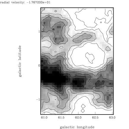
Figure 6: The shell GS62.1+0.2-18 in a velocity channel ($v_{\mathrm{LSR}}=-17.7\ \mathrm{kms^{-1}}$) and the $bv$ cut ($l=62.13^{\degr}$). The grey scale goes from white (the lowest temperature) to black (the highest temperature). The range of temperatures in the left panel is (7.3 K, 79.1 K), contour values are 14.5 (3.6) 72.0 K; in the right panel the range is (3.7 K, 92.9 K), contour values are 12.6 (4.5) 84.0 K.

This is a comparatively spherical shell in the outer Galaxy (see Fig. 6); it lies at a distance of 9.6 kpc. Its radius is 40 arcmin, or $\sim 110\ \mathrm{pc}$ (in the $l$ direction it is 120 pc, 100 pc in the $b$ direction). The expansion velocity is 13 $\mathrm{kms}^{-1}$. Only one wall is seen reliably. Table 3 summarizes properties of the shell.

One or more probably several supernovae were needed to create the shell GS62.1+0.2-18; its age is $\sim 5$ Myr.

4.5 GS60.0-1.1-54

$l$	$b$		$N_{\mathrm{{H\textsc{i}}\leavevmode\nobreak\ }}$	FWHM
			$\mathrm{cm^{-2}}$	$\mathrm{kms^{-1}}$
$60.0^{\degr}$	$+0.2^{\degr}$	hole	$2.6\times 10^{20}$	8.3
		wall	$4.5\times 10^{19}$	5.0
$60.0^{\degr}$	$-0.5^{\degr}$	hole	$3.6\times 10^{20}$	11.0
		wall 1	$2.4\times 10^{19}$	2.7
		wall 2	$9.3\times 10^{19}$	5.5
$60.1^{\degr}$	$-1.1^{\degr}$	hole	$5.1\times 10^{19}$	7.8
		wall	$3.9\times 10^{20}$	8.2

Table 4: GS60.0-1.1-54: $l$ and $b$ are coordinates of the spectrum taken through the structure, FWHM is the width of the line, $\mathrm{N_{{H\textsc{i}}\leavevmode\nobreak\ }}$ is the column density of H i swept up into the wall or missing in the hole.

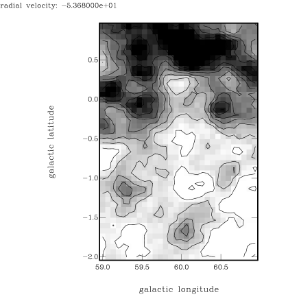
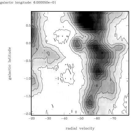
Figure 7: The shell GS60.1-1.1-54 in a velocity channel ($v_{\mathrm{LSR}}=-53.7\ \mathrm{kms^{-1}}$) and the $bv$ cut ($l=60.0^{\degr}$). The grey scale goes from white (the lowest temperature) to black (the highest temperature). The range of temperatures in the left panel is (6.3 K, 59.4 K), contour values are 11.6 (2.7) 54.0 K; in the right panel the range is (2.4 K, 56.9 K), contour values are 7.8 (2.7) 51.5 K.

The shell GS60.0-1.1-54 is a highly non-spherical structure (Fig. 7). It consists of a roughly spherical hole centered on ($60{\degr},0.2{\degr}$), connected with a cone which opens to the halo, closed by an arc. The shell lies in the outer Galaxy, at a distance of 13.7 kpc. Its dimensions are about $2{\degr}$ (500 pc) in the $b$-direction, the maximum diameter in the $l$-direction is $1.7{\degr}$ (400 pc). Though it is quite extended in the $b$-direction, it is not an object in the Koo et al. (1992) catalog of galactic worm candidates.

The H i shell GS60.0-1.1-54 is an irregular structure, however, it is probably not unique in the Milky Way. Its shape and dimensions are similar to the Aquila supershell (Maciejewski et al., 1996). For a possible scenario how to create such a structure compare the rightmost panel of Fig. 3 in Korpi et al. (1999) showing results of MHD simulations. The structure shown resembles the observations quite well, both in shape and dimensions.

The shell GS60.0-1.1-54 does not show the approaching hemisphere, i.e. it is open at one side (or the wall is negligible). The receding hemisphere is visible: the small “hole” around $(60.0^{\degr},+0.2^{\degr})$ changes diameter as expected from the expanding structure with an expansion velocity of 9 $\mathrm{kms^{-1}}$. The spectrum through $(60.0^{\degr},-0.5^{\degr})$ also shows the expansion (17 $\mathrm{kms^{-1}}$). The different expansion velocities are quite consistent with the idea that the fastest deceleration of the shell takes place in the densest part of the Galactic disk. The blown-out part at high latitudes changes shape and dimensions with velocity, though not in a very regular way. The best estimate of the expansion velocity is 9 $\mathrm{kms^{-1}}$. Table 4 gives the column densities in different positions inside the shell.

The shell GS60.0-1.1-54 is very irregular and therefore we have not estimated its energy, as this is very unreliable.

5 H i observations of H ii regions

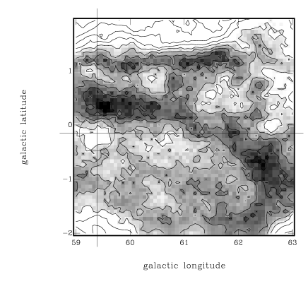
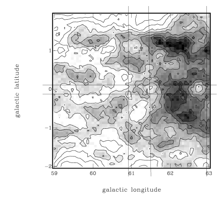
Figure 8: H ii regions in the observed field. The pixel map is the H i column density between $v_{\mathrm{LSR}}\in(+25,+33)\ \mathrm{kms}^{-1}$ with the S86 region (left panel); H i in $v_{\mathrm{LSR}}\in(+20,+25)\ \mathrm{kms}^{-1}$ with regions (from left to right) S87, S88 and S89 (right panel). Positions of H ii regions are indicated by big crosses and circles corresponding to dimensions of regions (S89 is very small, with the diameter only barely exceeding the size of the pixel, it lies near to the edge of the map at the upper cross-section of the lines). The grey scale goes from white (the lowest column density) to black (the highest density). The range of densities is in the left panel ($5.19\times 10^{20}\mathrm{cm}^{-2}$, $1.67\times 10^{21}\mathrm{cm}^{-2}$), contour values are $6.34\times 10^{20}$ ($1.15\times 10^{20}$) $1.55\times 10^{21}\mathrm{cm}^{-2}$; in the right panel the range is ($3.75\times 10^{20}\mathrm{cm}^{-2}$, $1.18\times 10^{21}\mathrm{cm}^{-2}$), contour values are $4.56\times 10^{20}$ ($8.05\times 10^{19}$) $1.10\times 10^{21}\mathrm{cm}^{-2}$.

There are four optical H ii regions in the observed field; S86, S87, S88 and S89 (Sharpless, 1959). We examine the distribution of the neutral hydrogen in their vicinity. Table 5 gives the properties of the four regions taken from Blitz & Fich (1982).

name	$l$	$b$	$\mathrm{v_{CO}}$ ($\mathrm{kms^{-1}}$)	$d$ (arcmin)
S86	$59.39^{\degr}$	$-0.15^{\degr}$	26.8	40
S87	$60.92^{\degr}$	$-0.13^{\degr}$	22.7	10
S88	$61.49^{\degr}$	$0.10^{\degr}$	22.9	25
S89	$62.94^{\degr}$	$0.11^{\degr}$	25.6	5

Table 5: H ii regions in the observed field. $l$ and $b$ are the coordinates of the centre, $v_{\mathrm{CO}}$ is the line-of-sight velocity of the CO counterpart of the optical region, $d$ is the diameter of the region.

5.1 S86

This H ii region is associated with the Vul OB1 association (NGC 6823). At the position of S86 there is a clear hole in the H i distribution, visible between $v_{\mathrm{LSR}}\in(+25,+31)\ \mathrm{kms}^{-1}$. The H ii region lies inside the hole, its dimensions are comparable to dimensions of the hole (see Fig. 8). The hole is stationary.

The coincidence of the H i hole and the H ii region is consistent with the idea, that most gas in the vicinity of the OB association is ionized and therefore not observed in 21 $\mathrm{cm}$ emission. The hole does not expand, which may mean, that no SN has exploded so far in the cluster (which is consistent with age estimates of NGC 6823: 2-7 Myr; Massey et al., 1995).

5.2 S87

S87 is a source observed in optical, infrared, radio recombination lines (RRL) and molecular line emission (Barsony, 1989; Onello et al. 1991). It has a compact core surrounded by an extended structure oriented south-east (i.e. perpendicular to the galactic plane). It interacts with a molecular cloud.

The H ii region S87 lies inside the hole in the H i distribution, visible between $v_{\mathrm{LSR}}\in(+20,+26)\ \mathrm{kms}^{-1}$. Again, this hole is stationary.

5.3 S88

S88 is also observed in RRLs, molecular line emission, infrared and optical (Wood & Churchwell, 1989; Onello et al., 1991). The region has an ultracompact core with a complex, multi-peaked structure.

S88 probably lies at the boundary between a dense sheet of gas and a more rarefied medium. At the position and the radial velocity of the region there is a small hole visible in a few velocity channels around $v_{\mathrm{LSR}}=23\ \mathrm{kms}^{-1}$, but definitely not as pronounced as in the case of S86 or S87. This hole is a part of the bigger empty region (see Fig. 8).

5.4 S89

S89 lies in a dense region (see Fig. 8). It is not situated inside any hole, at least not in the predicted velocity range, but it lies just on the edge of a small hole, visible between $v_{\mathrm{LSR}}\in(+20,+25)\ \mathrm{kms}^{-1}$. The physical association of these two structures, an H ii region and an H i hole, is unclear, but cannot be excluded.

5.5 Summary

In two out of four cases (S86, S87) we find a clear trace of the Strömgren sphere in the H i distribution, i.e. a stationary hole. In one case (S88) the connection H ii region – H i hole was not very obvious — there are depressions at the position of the region, but nothing really convincing. Maybe simply the gas distribution in the vicinity of S88 is so chaotic, that the nice Strömgren sphere does not exist. The region S89 does not lie inside a hole, but on the edge of one.

The chance coincidence of unrelated H ii regions and H i holes cannot be excluded, because of the distance ambiguity, but at least for S86 and S87 the probability of this coincidence is small, as not only the positions and radial velocities, but also the dimensions of H ii regions and H i holes agree.

The area where all these H ii regions lie, i.e. $v_{\mathrm{LSR}}\in(+10,+30)\ \mathrm{kms}^{-1}$, is a very turbulent region, full of structures on many scales (in Ehlerová, 2000, it was described as a strange kind of a complex, multicomponent H i shell GS60.1-0.3+15). This is partly the reason why none of the H i holes mentioned was identified as an independent H i shell.

6 Discussion — Summary

The $4{\degr}\times 4{\degr}$ field contains a rich variety of structures. Due to its limited size, selection effects play heavily against any statistical or general considerations and we can only describe individual structures.

• We reidentified Heiles’ supershell GS061+00+51. We confirm the previously ’detected’ properties (size, expansion velocity), though its morphology is more complex than was known before.

• We found two young spherical expanding shells GS59.9-1.0+38 and GS59.7-0.4+44 (with $R_{\mathrm{sh}}\sim 30\ \mathrm{pc}$ and $v_{\mathrm{exp}}\sim 10\ \mathrm{kms^{-1}}$). In the future they might merge with one another (in about 1 Myr) and later (3-4 Myr) with a bigger shell GS061+00+51 which is close by.

• Another regular elliptical shell GS62.1+0.2-18 was identified in the outer Galaxy.

• An irregular shell GS60.0-1.1-54 was found. This shell blows out from the Galactic disk. This behaviour is expected from H i supershells, but this structure lies in the outer Galaxy, where we do not expect any significant star formation and where the gaseous disk is thick.

• The initial density of the neutral hydrogen at positions of H i shells is in all cases higher than the average value; the typical $n_{0}$ is around 1 $\mathrm{cm^{-3}}$.

Apart from the described H i shells, which we consider to be non-turbulent structures (i.e. created by something else than purely by the turbulence, most probably by the activity of massive stars), there are other objects, which are less “homogeneous”, such as holes in the H i distribution connected with H ii regions (examples: H ii regions S86 and S87). However, we are not always able to connect the features in the H i with features in H ii (S88 and maybe also S89). Chaotic holes, arcs and sheets seen in our observations seem to be turbulent structures with no direct connection to physical objects.

Summing up, it seems that there are two types of “shell-like” structures found in the H i distribution. The first, formed by consistent structures, that are coherent in the position-velocity space, is less abundant than the second type, which contains non-coherent objects. We believe that these second type structures are created mainly due to the turbulence in the ISM. We identify the first group of objects with structures known as H i shells, as they fulfill the usual criteria put on shells. This is good news concerning the question about the existence of H i shells. The bad news is the fact that there is no well-defined boundary between the two types of structures.

- (1) Barsony M. 1989, ApJ, 345, 268
- (2) Blitz L., & Fich M. 1982, ApJS, 49, 183
- (3) Chevalier R. 1974, ApJ, 188, 501
- (4) Ehlerová S. 2000, PhD Thesis, Charles University, Prague
- (5) Hartmann D., & Burton W.B. 1997, Atlas of Galactic Neutral Hydrogen, Cambridge University Press
- (6) Heiles C., 1979 ApJ, 229, 533
- (7) Kalberla P.M.W., Mebold U., & Reif K. 1982, A&A, 106,190
- (8) Katgert P. 1969, AA, 1, 54
- (9) Koo B., Heiles C., & Reach W.T. 1992, Apj, 390, 108
- (10) Korpi M.J., Brandenburg A., Shukurov A., & Tuominen I. 1999, A&A, 350, 230
- (11) Maciejewski W., Murphy E.M., Lockmann F.J., & Savage B.D. 1996, ApJ, 469, 238
- (12) Massey P., Johnson K.E., & DeGioia-Eastwood K. 1995, ApJ, 454, 151
- (13) Onello J.S., Phillips J.A., & Terzian Y. 1991, ApJ, 383, 693
- (14) Sedov L. 1959, Similarity and Dimensional Methods in Mechanics, Academy Press, New York
- (15) Sharpless S. 1959, ApJS, 4, 257
- (16) Walter F., & Brinks E. 1999, AJ, 118, 273
- (17) Weaver H., & Williams D.R.W. 1973, A&AS, 8, 1
- (18) Wood D.O.S., & Churchwell E. 1989, ApJS, 69, 831
- (19) Wouterloot J.G.A., Brand J., Burton W.B., & Kwee K.K. 1990, A&A, 230,21