An Efficient Algorithm for Positioning Tiles
in the Sloan Digital Sky Survey

Abstract

The Sloan Digital Sky Survey (SDSS) will observe around $10^{6}$ spectra from targets distributed over an area of about 10,000 square degrees, using a multi-object fiber spectrograph which can simultaneously observe 640 objects in a circular field-of-view (referred to as a “tile”) 1.49^∘ in radius. No two fibers can be placed closer than $55^{\prime\prime}$ during the same observation; multiple targets closer than this distance are said to “collide.” We present here a method of allocating fibers to desired targets given a set of tile centers which includes the effects of collisions and which is nearly optimally efficient and uniform. Because of large-scale structure in the galaxy distribution (which form the bulk of the SDSS targets), a naïve covering the sky with equally-spaced tiles does not yield uniform sampling. Thus, we present a heuristic for perturbing the centers of the tiles from the equally-spaced distribution which provides more uniform completeness. For the SDSS sample, we can attain a sampling rate of $>92\%$ for all targets, and $>99\%$ for the set of targets which do not collide with each other, with an efficiency $>90\%$ (defined as the fraction of available fibers assigned to targets).

1 Introduction

The Sloan Digital Sky Survey (SDSS; York et al. 2000) is producing a deep imaging survey over about 10,000 square degrees, using a camera with a large format CCD array on a dedicated telescope at Apache Point Observatory in New Mexico (Gunn et al. 1998). A sample of objects selected from this imaging survey is being targeted for a spectroscopic follow-up survey which is being conducted concurrently. About 900,000 of these spectroscopic targets will be galaxies (Strauss et al. 2001), about 100,000 will be QSOs (Richards et al. 2001), and about 100,000 will be selected by color to be intrinsically very red, luminous galaxies known as “Luminous Red Galaxies” (Eisenstein et al. 2001). In this paper, we will refer to all of these objects generically as “tiled targets,” or often simply “targets.”

These targets are observed using two multi-object fiber spectrographs on the same telescope (Uomoto et al. 2001). Each spectroscopic fiber plug plate, referred to as a “tile,” has a circular field-of-view with a radius of 1.49^∘ and can accommodate 640 fibers, 48 of which are reserved for observations of blank sky and spectrophotometric standards. Because of the finite size of the fiber plugs, the minimium separation of fiber centers is $55^{\prime\prime}$. If, for example, two objects are within $55^{\prime\prime}$ of each other, both of them can be observed only if they lie in the overlap between two adjacent tiles. Simulations and early observations both suggest that 10% of targets in the SDSS will be unobservable if they do not lie in overlaps of tiles; about 30% of the sky will be covered by such overlaps. The goal of the SDSS is to observe $99\%$ of the maximal set of targets which has no such collisions (about 90% of all targets). In Section 4 we give a more complete description of the details of the SDSS.

Around 2,000 tiles will be necessary to provide fibers for all the targets in the survey. Since each tile which must be observed contributes to the cost of the survey (due both to the cost of production of the plate and to the cost of observing time), we desire to minimize the number of tiles necessary to observe all the desired targets. In order to maximize efficiency (defined as the fraction of available fibers assigned to tiled targets) when placing these tiles and assigning targets to each tile, we need to address two problems. First, we must be able to determine, given a set of tile centers, how to optimally assign targets to each tile — that is, how to maximize the number of targets which have fibers assigned to them. This problem is non-trivial because the circular tiles overlap. Second, we must determine the most efficient placement of the tile centers, which is non-trivial because the distribution of targets on the sky is non-uniform, due to the well-known clustering of galaxies on the sky. It turns out that the first problem can be solved in polynomial time, even in the presence of fiber collisions (as long as targets are distributed across the sky in a reasonable way). The second problem belongs to a class of problems for which only exponentially expensive methods for finding the exact solution are known (that is, it is “$NP$-complete”), but we use a heuristic method developed by Lupton, Maley, & Young (1998) to find an approximate solution.

This paper discusses the strategy used by the SDSS to place its tiles using these methods. It is designed to run on a patch of sky consisting of a set of rectangles in a spherical coordinate system, known in SDSS parlance as a “chunk.” Much of the strategy was described by Lupton, Maley, & Young (1998); this paper provides more astronomical context and describes the method for resolving fiber collisions. Section 2 describes the method. Section 3 shows example results from actual SDSS data and from simulations. Section 4 describes some technical aspects of the SDSS. Section 5 summarizes our results.

2 Tile Placement and Fiber Allocation

Here we describe our method for placing each tile and allocating the fibers of each tile to the targets. First, we discuss the allocation of fibers given a set of tile centers. In the absence of fiber collisions, this problem can be solved quickly and optimally, as shown in Section 2.1. A method which is nearly optimal in the presence of fiber collisions is presented in Section 2.2. Second, in Section 2.3, we discuss how to efficiently place the centers of the tiles.

2.1 Target-to-Tile Assignment without Collisions

Given a distribution of targets on the sky and an a priori set of tile centers, one can find the optimal solution to the problem of allocating the targets to each tile, such that the maximum possible number of targets are assigned fibers. With circular tiles, which necessarily overlap, this is a somewhat non-trivial problem.

Figure 1 shows at the top a very simple example of a distribution of targets and the positions of two tiles we want to use to observe these targets. Given that for each tile there is a finite number of available fibers, how do we decide which targets get allocated to which tile? As realized by Lupton, Maley, & Young (1998), this problem is equivalent to a network flow problem, which computer scientists have been kind enough to solve for us already (e.g., Goldberg 1997).

The basic idea is shown in the bottom half of Figure 1, which shows the appropriate network for the situation in the top half. Using this figure as reference, we here define some terms which are standard in combinatorial literature and which will be useful here:

• node: The nodes are the solid dots in the figure; they provide either sources/sinks of objects for the flow or simply serve as junctions for the flow. For example, in this context each target and each tile corresponds to a node.

• arc: The arcs are the lines connecting the nodes. They show the paths along which objects can flow from node to node. In Figure 1, it is understood that the flow along the arc proceeds to the right. For example, the arcs traveling from target nodes to tile nodes express which tiles each target may be assigned to.

• capacity: The minimum and maximum capacity of each arc is the minimum and maximum number of objects that can flow along it. For example, because each tile can accommodate only 592 fibers, the capacities of the arcs traveling from the tile nodes to the sink node is 592.

• cost: The cost per object along each arc is exacted for allowing objects to flow down a particular arc; the total cost is the summed cost of all the arcs. In this paper, the network is designed such that the minimum total cost solution is the desired solution.

Imagine that you have a flow of 7 objects which enters the network at the source node at the left. The goal is for the entire flow to leave the network at the sink node at the right for the lowest possible cost. The objects must travel along the arcs, from node to node. Each arc has a maximum capacity of objects which it can transport, as labeled. (One can also specify a minimum number, which will be useful later). Each arc also has an associated cost, which is exacted per object which is allowed to flow across that arc. Arcs link the source node to a set of nodes corresponding to the set of targets. Each target node is linked by an arc to the node of each tile it is covered by. Each tile node is linked to the sink node by an arc whose capacity is equal to the number of fibers available on that tile. None of these arcs has any associated cost. Finally, an “overflow” arc links the source node directly to the sink node, for targets which cannot be assigned to tiles. The overflow arc has effectively infinite capacity; however, a cost is assigned to objects flowing on the overflow arc, guaranteeing that the algorithm fails to assign targets to tiles only when it absolutely has to. This network thus expresses all the possible fiber allocations as well as the constraints on the numbers of fibers in each tile. Finding the minimum cost solution (which can be done in polynomial time using the method of Goldberg 1997) then maximizes the number of targets which are actually assigned to tiles.

However, there are a couple of properties of the network flow solutions which must be treated with caution. First, notice that in this example there are only three types of target nodes: those only in tile 1, those only in tile 2, and those in both. When the network flow algorithm we use here chooses its solution, it does not guarantee that it chooses targets within each of these types randomly. Thus, if the order of the target nodes as sent to the network flow algorithm are correlated with any target property (for example, position on the sky), the distribution of that property in targets assigned to tiles will differ from the distribution in all of the targets. Take for example the situation that the targets are sorted by right ascension. If the algorithm is unable to assign fibers to some of the targets, it is likely that the unassigned targets will be nodes that are close to each other in Figure 1. Therefore, they will also be clumped in right ascension. This is unacceptable if we desire a reasonable window function. Thus, we randomize the order in which nodes are assigned to targets by this algorithm; this prevents any correlation between target properties and whether a target gets a fiber.

Second, the particular method we use, provided by Goldberg (1997), has the interesting property that when a certain number of targets cannot be allocated fibers, the algorithm preferentially chooses to exclude targets which are covered by more than one tile. This property has no effect on the overall efficiency of the solution, but because the method for fitting for tile positions presented in Section 2.3 will tend to put overlaps of tiles in preferentially overdense regions, it may introduce subtle correlations between the sampling rate and the density field. This behavior is important if the level of completeness in low is parts of the tiling region; however, the uniformity of our completeness is high enough that this effect is not important.

2.2 Target-to-Tile Assignment with Collisions

As described above, there is a limit of $55^{\prime\prime}$ to how close two fibers can be on the same tile. If there were no overlaps between tiles, these collisions would make it impossible to observe $\sim 10\%$ of the SDSS targets. Because the tiles are circular, some fraction of the sky will be covered with overlaps of tiles, allowing some of these targets to be recovered. In the presence of these collisions, the best assignment of targets to the tiles must account for the presence of collisions, and strive to resolve as many as possible of these collisions which are in overlaps of tiles. We approach this problem in two steps, for reasons described below. First, we apply the network flow algorithm of Section 2.1 to the set of “decollided” targets — the largest possible subset of the targets which do not collide with each other. Second, we use the remaining fibers and a second network flow solution to optimally resolve collisions in overlap regions.

2.2.1 Network Flow for Decollided Objects

The effect of fiber collisions is one which any analysis of the SDSS data is going to face. The fact that most ($70\%$) of the sky in the survey will be only covered by a single tile means that a certain number of objects will be missed for this reason. Thus, the best that one can hope for in terms of sampling is that all unobserved targets have a close neighbor which was observed; the redshift of the observed target would thus give us some prior information on the redshift of the unobserved target. Furthermore, exactly where and how many targets one can recover in tile overlaps depends strongly on the locations of the tiles, and thus on the target density field. To evaluate the effect of this dependence on large-scale structure statistics, one would have to run the algorithm described here on a large number of mock catalogs. For these two reasons, we must take care that we identify a set of targets which we could observe no matter where the tiles are, and obtain as complete a sample as possible of these targets.

To identify this sample, we define the maximal subset of the targets which are all greater than $55^{\prime\prime}$ from each other, which we refer to as the “decollided” set. To clarify what we mean by this maximal set, consider Figure 2. Each circle represents a target; the circle diameter is $55^{\prime\prime}$, meaning that overlapping circles are targets which collide. The set of solid circles is the “decollided” set. Thus, in the triple collision at the top, it is best to keep the outside two rather than the middle one. To find this decollided set of targets, we run a friends-of-friends grouping algorithm on the targets with a $55^{\prime\prime}$ linking length. The resulting groups are almost always of sufficiently low multiplicity that we can simply check all possibilities to find the best possible selection of targets which eliminates fiber collisions. We pick at random one of the set of equivalent “best” selections; for example, if two objects collide, this algorithm simply picks one at random to be “decollided.”

This determination is complicated slightly by the fact that some targets are assigned higher priority than others. For example, as explained in Section 4.1, QSOs are given higher priority than galaxies by the SDSS target selection algorithms. What we mean here by “priority” is that a higher priority target is guaranteed never to be eliminated from the sample due to a collision with a lower priority object. Thus, our true criterion for determining whether one set of assignments of fibers to targets in a group is more favorable than another is that a greater number of the highest priority objects are assigned fibers. In the case of a tie in the highest priority objects, the next highest priority objects are considered, and so on.

Once we have identified our set of decollided objects, we use the network flow solution to find the best possible assignment of fibers to that set of objects.

2.2.2 Network Flow for Collisions

After allocating fibers to the set of decollided targets, there will usually be unallocated fibers, which we want to use to resolve fiber collisions in the overlaps. We can again express the problem of how best to perform the collision resolution as a network, although the problem is a bit more complicated in this case. In the case of binaries and triples, we design a network flow problem such that the network flow solution chooses the tile assignments optimally. In the case of higher multiplicity groups, our simple method for binaries and triples does not work and we instead resolve the fiber collisions in a random fashion; however, fewer than 1% of targets are in such groups, and the difference between the optimal choice of assignments and the random choices made for these groups is only a small fraction of that.

The design of the second network flow is similar to the first, with source and sink nodes (connected by the overflow arc) and a layer of tile nodes. However, instead of a layer of target nodes, we have a layer of nodes corresponding to each group (as defined by the aforementioned friends-of-friends algorithm) which has at least one member in an overlap of tiles. We thus ignore groups covered only by one tile, since we have already done as well as possible for those targets. Note we include single-member groups in this process, which allows targets in overlaps which were previously guaranteed a fiber on one plate to be shuffled to another plate, if it proves desirable to do so.

First, we need to set the properties of each arc connecting the source node to each group node. For each group, we find the maximum number of targets which could be observed, $c_{\mathrm{max}}$, taking advantage of the overlapping tiles, but regardless of the number of available fibers in each tile. We find $c_{\mathrm{max}}$ by simply trying all possible target-to-tile configurations for that group, and picking the best solution (again accounting for the relative priorities of the objects). A constraint on the best solution is that some subset of the targets in each group will have been allocated fibers as decollided targets in the first network flow. Any “best” solution must guarantee that these targets will be assigned fibers again in the second network flow. In addition, these required targets clearly set a minimum number of targets to observe in each group, $c_{\mathrm{min}}$. Each source-to-group arc will have its maximum and minimum capacity set according to these bounds.

Second, we need to set the properties of each arc connecting a group node to a tile node. In the case that $c_{\mathrm{max}}\leq 3$, we determine the maximum number of targets which can be assigned to each tile, $c_{\mathrm{max},i}$, given all the equivalent “best” sets of target-to-tile assignments. The minima $c_{\mathrm{min},i}$ are set to the minimum number of arcs in each tile, given all legal target-to-tile assignments. The group-to-tile arcs are then assigned these maximum and minimum capacities. Under these conditions, in almost every case, any solution the network flow finds will be achievable, in the sense that it can be implemented without the occurrence of fiber collisions. See below for a discussion of the exceptions.

In the case that $c_{\mathrm{max}}>3$, the same prescription does not provide the assurance that the network flow will return a viable set of tile assignments, and instead we pick a particular “best” set of target-to-tile assignments for each such group in order to guarantee feasibility. In this case, the code chooses at random a particular realization of the “best” resolution of the fiber collisions, (one must also be careful, in the $c_{\mathrm{max}}>3$ case, to guarantee fibers to all of the decollided fibers which were picked in the first network flow solution; this task is complicated but tractable).

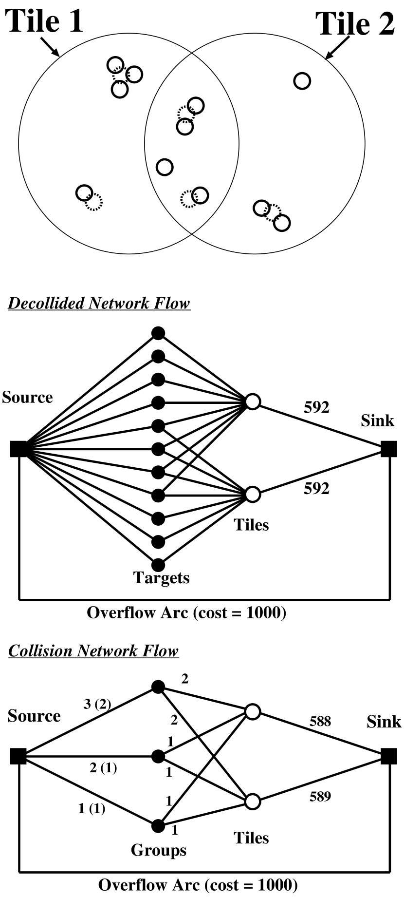
Figure 3: Top panel shows a schematic distribution of targets and tiles, as in Figure 1; in the manner of Figure 2, the decollided galaxies are solid circles and the others are dashed circles. Middle panel shows the decollided network flow (Section 2.2.1) used to find the optimal solution for decollided objects; this network flow has the same form as that in Figure 1 (here unmarked arcs have a capacity of unity). Bottom panel shows the network flow used to resolve collisions in overlaps of tiles. In this case, the set of target nodes has been replaced by nodes corresponding to each group with one or more members in an overlap of tiles. For the case shown here, there are three such groups. The arcs to and from each group have minimum and maximum capacities set as described in the text. If omitted, the maximum capacity is unity. The minimum capacity for each arc is put in parentheses after the maximum; if omitted, the minimum capacity is zero.

For the sake of concreteness, consider Figure 3, which shows a possible tile-target configuration and the networks which would be constructed to solve it. Again, the solid circles indicate the “decollided” set of targets, which has 11 members, and for which the decollided network flow is run (unmarked arcs have a capacity of unity). Assuming all the decollided targets are obtained, we set up the network flow for the groups in the overlap as shown at the bottom. Each source-to-group arc is marked by its maximum capacity $c_{\mathrm{max}}$ followed by its minimum capacity $c_{\mathrm{min}}$ in parentheses. As explained above, these minima are set by the fact that some of the targets are guaranteed spots because they were previously assigned tiles in the decollided solution. The group-to-tile capacities are set to the maximum possible on any given tile. Again, setting things up this way allows the network flow solution to optimally allocate the overlap fibers (at least for triples and binaries) while still guaranteeing that a solution is possible and that fibers are assigned to all the decollided targets which had been previously selected.

As mentioned above, there are cases for which these rules return unfeasible answers. Under the conditions of the SDSS, these cases are extraordinarily rare; we mention them because the same may not be true for every application. There are essentially two classes of failures. First, occasionally it happens that because part of a group is in an overlap and part is not, the “best” solution requires that more fibers be assigned to a tile than were assigned in the decollided solution. If, in conjunction with this occurrence, the tile in question is in a particularly dense region, it may already require all its fibers to cover the decollided targets. Thus, applying the rules above creates a second network flow with no possible solution. In such cases, the code reverts to a “fail-safe” mode which only allows solutions to the group-to-tile problem which put the same number of decollided targets onto each tile as were assigned in the first network flow.

Second, and again very rarely, it occasionally happens that while the second network flow successfully returns a choice of fiber assignments, this choice makes it impossible to assign fibers to all the decollided targets which were guaranteed fibers in the first network flow, not because of a lack of fibers but because of geometrical considerations. Again, the problem is associated with groups which straddle tile boundaries. In this case, the problem occurs when some targets in a group are in an overlap of three or more tiles, and others to be in an overlap of a lesser number of tiles. In the code, we simply warn the user that some decollided targets have been lost. On the basis of simulations, we expect ten to twenty of the million SDSS targets to be lost due to this effect.

2.3 Tile Placement

Once one understands how to assign fibers given a set of tile centers, one can address the problem of how best to place those tile centers. One can show that to solve this problem optimally is $NP$-hard (e.g. Megiddo & Supowit 1984), but Lupton, Maley, & Young (1998) have developed a heuristic method which works well for the sorts of distributions of targets we deal with here. This method first distributes tiles uniformly across the sky and then uses a cost-minimization scheme to perturb the tiles to a more efficient solution.

2.3.1 Initial Conditions

We need to choose some initial, nearly uniform covering of the region to be tiled, before perturbing it to improve the efficiency. We use two techniques. First, for sufficiently large chunks of sky, we draw the uniform tiling from an approximately uniform covering of the sphere provided by Hardin, Sloane & Smith (2001). These coverings are provided for discrete numbers of tiles; the choice appropriate for the SDSS target density (about 120 per square degree) is 7682 tiles over the whole sky. We throw away tiles whose centers are not in the chunk of sky of interest to us. Second, for smaller chunks of sky (which a small chunk of the uniform spherical covering is less likely to cover in a reasonable way) we simply lay down a rectangle of tiles, with the centers of the tiles in each row offset in order to provide a complete covering.

2.3.2 Perturbing the Tiles

The method is essentially iterative. One starts with a uniform covering of tiles over the region in question, as described in the previous subsection. Then, one allocates targets to the tiles, but instead of limiting a target to the tiles within a tile radius, one allows a target to be assigned to further tiles, but with a certain cost which increases with distance (remember that the network flow accommodates the assignment of costs to arcs). For group-to-tile nodes in the second network flow solution, one defines the cost according the position of the group center. One uses exactly the same fiber allocation procedure as above.

In practice, we do not allow fibers to be assigned to any tile, but only those within $2.5$ times the tile radius. We assign a cost of the following form:

$$c=\begin{array}[]{cc}0&r<R_{\mathrm{tile}}\cr A\left[\left(\frac{r}{R_{\mathrm{tile}}}\right)^{\alpha}-1\right]&r>R_{\mathrm{tile}}\end{array},$$ (1)

where $r$ is the distance of the fiber from the center of the tile, $R_{\mathrm{tile}}$ is the radius of the tile, and $\alpha$ is the logarithmic slope of the cost function. $A$ is a scale factor, set so that at $r=2.5R_{\mathrm{tile}}$ the cost is equal to the cost of not assigning the fiber at all.

What this does is to give each tile some information about the distribution of targets outside of it. Then, once one has assigned a set of targets to each tile, one changes each tile position to that which minimizes the cost of its set of targets. To perform this minimization, we use Powell’s direction set method, as described by Press et al. (1992). Then, with the new positons, one reruns the fiber allocation, perturbs the tiles again, and so on. As Lupton, Maley, & Young (1998) point out, this method is guaranteed to converge to a minimum (though not necessarily a global minimum), because the total cost must decrease at each step.

The parameter $\alpha$ sets the slope of the cost function; the most advantageous value of $\alpha$ depends in detail on the density and distribution of the targets. We generally set $0.5<\alpha<2$. High values in this range encourage tiles to take large excursions from their initial positions, since the slope of the cost function becomes higher at larger radii. Under these conditions, tiles are influenced by distant targets that they may never cover; however, this behavior can be desirable for large chunks of sky for which the best solution may require large numbers of tiles to shift in unison. Low values in this range are more conservative in the sense that tiles are encouraged to travel less far from their initial positions, since the slope of the cost function decreases with radius. This behavior is usually desirable for small chunks of sky, for which many tiles are sitting near an edge and large changes of position will usually uncover sky. Perhaps a more general approach is to allow $\alpha$ to be variable in some way throughout the minimization.

Depending on the overall survey goals, one can choose to which set of targets these costs apply. For the SDSS, we are most interested in maximizing the fraction of decollided targets which are observed. For this reason, we assign cost only to the decollided targets, effectively ignoring the other objects when fitting for tile positions. In fact, during the iteration we do not even perform the second network flow.

It is possible to assign fibers to a slightly larger fraction (by about $1\%$) of all targets if all targets are included in the cost minimization. However, for the SDSS this improvement would come at the cost of large numbers of gaps opening up between tiles, because the number of tiles necessary to observe all the targets is uncomfortably close to the number of tiles necessary to simply cover the available sky. This effect highlights an important facet of the tiling problem: inefficiency arises because tiles which are in underdense regions cannot always be moved towards dense regions without leaving parts of the sky completely uncovered. A much higher target (and thus tile) density would mitigate this difficulty.

In practice, we also need to determine the appropriate number of tiles to use. Thus, using a standard binary search, we repeatedly run the cost-minimization to find the minimum number of tiles necessary to satisfy the SDSS requirements, namely that we assign fibers to $>99\%$ of the decollided targets.

3 Testing the Method

In order to test how well this algorithm works, we apply it both to simulated and real data. First, we test the algorithm on a large solid angle sample drawn from an $N$-body simulation. Second, we show results based on actual tiling solutions for a small chunk of sky in the SDSS commissioning data.

3.1 Simulation Tests

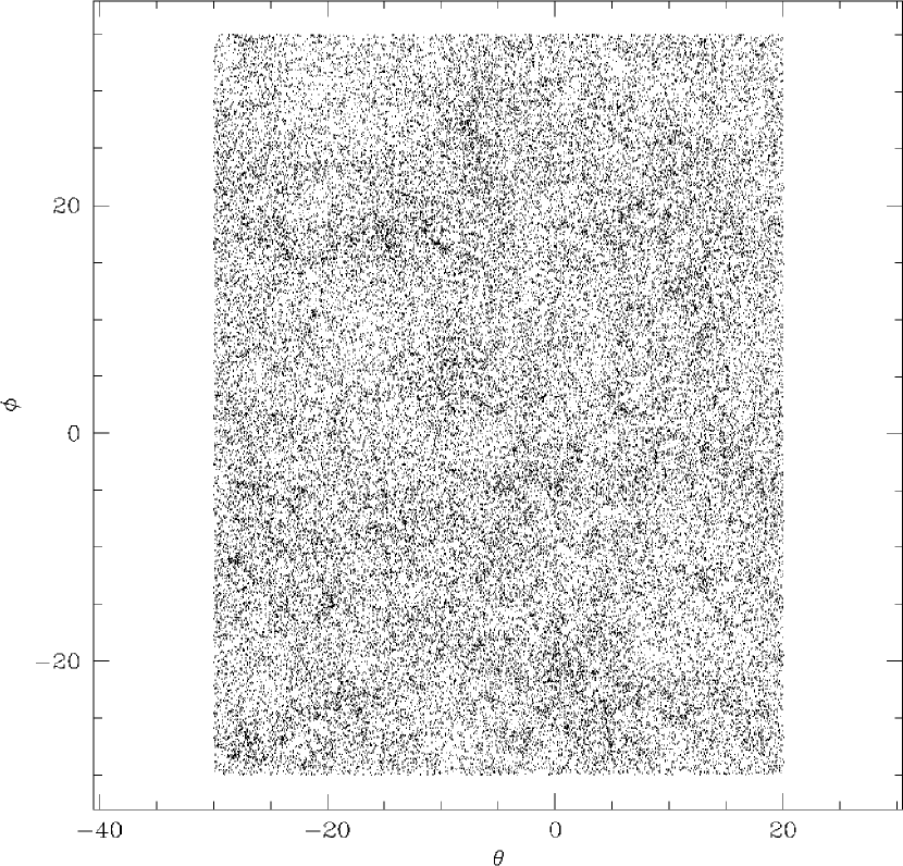
Figure 4: Distribution of targets on the sky, using galaxies drawn from a simulation by Cole et al. (1998), plus 20 targets per square degree added randomly to represent LRG and QSO targets. We have subsampled the targets by a factor of five for this plot.

For this exercise, we use the simulations of Cole et al. (1998), which are collisionless $N$-body simulations of the growth of structure in a COBE-normalized Cold Dark Matter (CDM) model with $\Omega_{m}=0.3$, $\Omega_{\Lambda}=0.7$, and $\sigma_{8}=1.05$. In this simulation, dark matter particles are chosen randomly to represent galaxies, and are assigned luminosities based on an assumed luminosity function. The location of an observer is chosen, a flux limit is assumed, and the galaxies in the simulation are “observed.” The resulting distribution of galaxies has about the same redshift distribution as do galaxies in the actual SDSS survey, with a median $z\sim 0.1$. This procedure results in a surface density (about 90 per square degree) and an angular clustering of galaxies on the sky approximately the same as the SDSS. In order to simulate the quasar and LRG samples, we distribute an extra 20 targets per square degree randomly on the sky; although in three dimensions both populations are highly clustered, their large distance and sparse sampling make the approximation that they are randomly distributed in angle not bad for our purposes. We extract a section of the simulation about 3075 square degrees in solid angle (a rectangle in spherical coordinates spanning the latitude range $-30^{\circ}<\theta<35^{\circ}$ and the longitude range $-30^{\circ}<\phi<20^{\circ}$) and consisting of 336,392 objects. The distribution of galaxies in this range is given in Figure 4. This angular region is probably larger than any that will be available during the course of the SDSS.

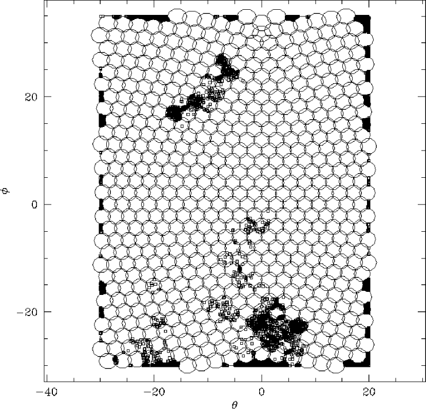
Figure 5: Results of distributing tiles uniformly across the targeted region. The boundaries of the tiles are shown. Missing decollided galaxies are shown as squares. While overall the completeness is high, note that in the densest regions, many decollided objects are missing, with the completeness becoming as low as 10% in the most incomplete regions.

As initial conditions for this large “chunk,” we extract a portion of a nearly uniform covering of the sphere given by Hardin, Sloane & Smith (2001). We exclude any tiles whose centers are outside the official boundaries of the chunk. This procedure will leave missing targets near the edges; these targets can be recovered when the adjacent region of sky is tiled. In any case, any gaps which are left when the survey is completed can be accounted for in the window function, to the extent that those gaps are uncorrelated with the underlying density of galaxies. For our first test, we do not perturb the positions of the tiles at all, and assign the fibers to the uniformly distributed tiles. The results are shown in Figure 5; here we show the tiles as circles and the missing decollided galaxies as squares. Decollided galaxies which were assigned fibers and all collided galaxies are omitted from the plot. The statistics associated with this solution are given in the first column of Table 1. It is clear that although the overall completeness is high ($\sim 98.3\%$ of decollided objects are assigned) the small amount of incompleteness is concentrated in a few, dense regions of sky. The patch of incompleteness near the bottom center is about 85–90% complete in the decollided objects on average; the most incomplete sections of that are only 10—30% complete. Clearly it is unsatisfactory to have such a high rate of incompleteness concentrated in unusually dense regions of sky, even if the overall completeness of the survey is high. Such a strong correlation of the sampling fraction with the galaxy density field poses difficulty estimating large-scale structure statistics.

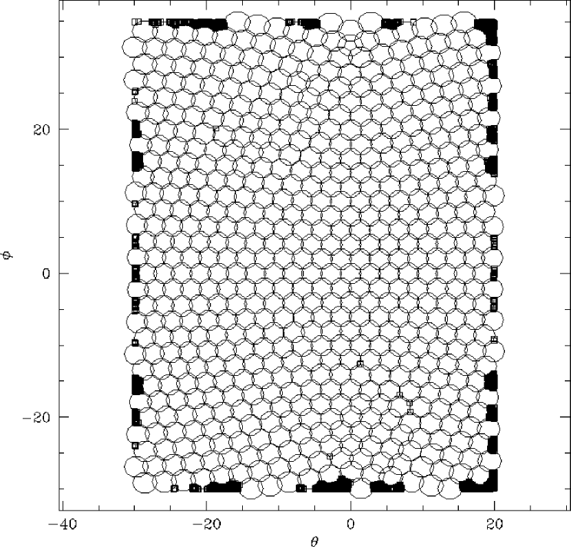
Figure 6: Same as Figure 5, now with the results of perturbing the positions of the tiles using the cost minimization heuristic described in Section 2.3.2. While the tiles move very little from their uniform initial distribution, the completeness has improved and has become far more uniform. Only a few objects are missing in the interior of the sample. This improvement occurs because in the densest regions tiles are pushed together, and thus overlap more.

Let us therefore perturb the tiles in an effort to increase the completeness and its uniformity. The result of applying the method described in Section 2.3 is shown in Figure 6; the resulting tiling statistics are given in the second column of Table 1. (Note that one extra tile was added in the process; this has a negligible effect on the statistics in Table 1). Now there are only a handful of objects missing in the interior of the sample. All of the missing objects are concentrated at the edges. Thus, while the overall completeness is increased a bit (to $\sim 99.0\%$ of decollided objects), the real improvement is in the uniformity of the sample.

To show how the resolution of collisions works, we show as points in Figure 7 the collided galaxies (those which are not in the decollided set). We have zoomed into a section of the interior to make it easier to distinguish the points. These points represent the set of objects which would be eliminated due to fiber collisions if there was no overlap between tiles. Open squares are placed over those which did not receive fibers. It is clear that in the underdense regions most of the collisions in overlaps of tiles are actually resolved. In the overdense regions, however, almost all of the fibers are used to observe decollided targets, and few are left over to resolve collisions.

Overall, in these simulations, $\sim 92.5\%$ of the available targets were assigned fibers; most of the missing ones are due to fiber collisions which were not able to be resolved. The efficiency of the tiling solution, quantified as the percentage of fibers which are used on tiled objects, is $\sim 91.2\%$.

3.2 Tests with SDSS Data

We here show tiling results using this method from SDSS commissioning data. In this phase of the survey, there was not enough imaging data yet to define a chunk as large as in the simulations of the previous subsection, so we had to settle for a much smaller chunk of sky. This chunk (known as “Chunk 7”) of sky is 5 degrees wide and about 12 degrees long, and contains 6629 objects. It is the first chunk of SDSS data on which this version of the code was used.

The initial conditions were set up simply as a rectangular distribution of tiles. The tile positions were perturbed in order to maximize the number of decollided galaxies assigned to fibers. However, in this case the tiles move very little — the uniform initial conditions turn out to be close to a minimum in our cost function. The statistics of the solution are listed again in Table 1; note that the efficiency is a bit low, mainly because this chunk is small. The positions of the targets and tiles are given in Figure 8.

An obvious criticism of the tiling of this chunk is that we should only tile the center of the chunk, such that our tiles never cover sky which has not yet been imaged. Then we would wait until later to observe edges of the chunk. In terms of the total number of tiles drilled, such an approach would be more efficient. However, doing this would leave the telescope idle when it could be taking spectra, so it is worth drilling a few more tiles than necessary in order to optimally use the available time. In any case, the fibers left unassigned to any main survey targets are assigned to other targets, mainly stars, FIRST (Becker, White, & Helfand 1995) sources, and ROSAT (Voges et al. 1999) sources, so the unassigned fibers are by no means wasted.

4 Technical Details for SDSS Data

There are a few technical details which may be useful to mention in the context of SDSS data, since understanding these issues is crucial to understanding the window function when calculating large-scale structure statistics with the survey. First, we will describe which targets within the SDSS are “tiled” in the manner described here, and how such targets are prioritized. Second, we will discuss the method used by SDSS to deal with the fact that the imaging and spectroscopy are performed within the same five-year time period. Third, we will describe the tiling outputs which the SDSS tracks as the survey progresses. Throughout, we refer to the code which implements the algorithm described above as tiling.

The information described in this section (along with the spectroscopic results) is necessary but not quite sufficient to calculate large-scale structure statistics for the survey. First, at later stages in the processing, fibers can be lost due to collisions with guide fibers, as well as with the center of the tile, where a post prevents any fiber from being placed within $100^{\prime\prime}$ (in later versions, we will adjust the algorithm described here to attempt to avoid placing tile centers so close to targets). Second, some fields within each chunk are excluded for reasons such as bad seeing. Finally, bright stars make it impossible to observe galaxies in a certain fraction of the sky, in a way which varies with Galactic latitude. These masks need to be determined to study clustering on the largest scales in the survey.

4.1 Targets Which are “Tiled”

Only some of the spectroscopic target types identified by the target selection algorithms in the SDSS are “tiled.” These types (and their designations in the primary and secondary target bitmasks, as described in Stoughton et al. 2001) are listed in Table 2. They consist of most types of QSOs, main sample galaxies, LRGs, hot standard stars, and brown dwarfs. These are the types of targets for which tiling is run and for which we are attempting to create a well-defined sample. Once the code has guaranteed fibers to all possible “tiled targets,” remaining fibers are assigned to other target types by a separate code.

All of these target types are treated equivalently, except that they assigned different “priorities,” designated by an integer. As described above, the tiling code uses them to help decide fiber collisions. The sense is that a higher priority object will never lose a fiber in favor of a lower priority object. The priorities are assigned in a somewhat complicated way for reasons immaterial to tiling, but the essense is the following: the highest priority objects are brown dwarfs and hot standards, next come QSOs, and the lowest priority objects are galaxies and LRGs. QSOs have higher priority than galaxies because galaxies are higher density and have stronger angular clustering. Thus, allowing galaxies to bump QSOs would allow variations in galaxy density to imprint themselves into variations in the density of QSOs assigned to fibers, which we would like to avoid. For similar reasons, brown dwarfs and hot standard stars (which have extremely low densities on the sky) are given highest priority.

Each tile, as stated above, is 1.49^∘ degrees in radius, and has the capacity to handle 592 tiled targets. No two such targets may be closer than 55^′′ on the same tile.

4.2 Definition of a Tiling Chunk

The modus operandi of the SDSS makes it impossible to tile the entire 10,000 square degrees simultaneously, because we want to be able to take spectroscopy during non-pristine nights, based on the imaging which has been performed up to that point. In practice, periodically a “chunk” of data is processed, calibrated, has targets selected, and is passed to the tiling code. During the first year of the SDSS, about one chunk per month has been created; as more and more imaging is taken and more tiles are created, we hope to decrease the frequency with which we need to make chunks, and to increase their size.

The first chunk which is “supported” by the SDSS is denoted Chunk 4. The first chunk for which the version of tiling described here was run is Chunk 7. Chunks earlier than Chunk 7 used a different (less efficient) method of handling fiber collisions. The earlier version also had a bug which artificially created gaps in the distribution of the fibers. The locations of the known gaps are given in Stoughton et al. (2001) for Chunk 4, since it is part of the SDSS Early Data Release.

A chunk is defined as a set of rectangles on the sky (defined in survey coordinates; Stoughton et al. 2001) on the sky. All of these rectangle are designed to cover only sky which has been imaged and processed. Most of each chunk consists of targets which have not been included in any previous chunk. However, if an earlier chunk was adjacent, targets may have been missed near its edges because they were not covered by tiles, so the areas near the edges of adjacent chunks are also included. Thus, in general, chunks overlap.

4.3 Tiling Outputs

Once a chunk is tiled, the position of each tile is stored. The tiles are assigned a global index for the survey known as a tileId. For each target, the tileId to which it is assigned is stored (or $-1$ if no fiber is assigned). In addition, the $55^{\prime\prime}$ group to which it belonged (indexed from 0 for each chunk independently) is also stored as collisionGroup. Finally, a mask parameter is created, whose three lowest bits are (respectively): ASSIGNED, DECOLLIDED, and COVERED. ASSIGNED means that a fiber was actually assigned to the target. DECOLLIDED means that the target was designated a decollided target. COVERED means that the target was in an area observable by some tile. Unfortunately, these parameters are not included in the SDSS Early Data Release.

5 Summary

This paper describes a method for positioning tiles and assigning fibers to targets which is being used for the SDSS. The method assigns fibers in a near-optimal manner, which is possible to do in polynomial time given the sorts of target distributions found in the SDSS. We note that if the typical nearest-neighbor distance of targets is of order the fiber collision length, the groups found in the friends-of-friends algorithm become very large, and the solution is only possible in exponential time. The positioning of tiles is an $NP$-complete problem (Megiddo & Supowit 1984); we use the heuristic devised by Lupton, Maley, & Young (1998) to find an approximate solution. Importantly, we define a set of decollided targets for which we can achieve nearly complete sampling; this fact will make the survey easier to mimic when analyzing simulations. We have tested this method both on simulations and on SDSS commissioning data. Finally, we have described some of the technical details of the SDSS itself.

Variations of this method may be useful for future surveys consisting of overlapping spectroscopic fields of view. The main lesson learned in developing this method is that inefficiencies arise primarily due to the need to completely cover the given area. To take the most perverse possible case, if 592 objects were spread across the entire sky, 592 tiles would be necessary. One would rather have those 592 targets within the area of a single tile, which could assign fibers to all of them. Thus, to minimize the number of tiles drilled, one needs a high enough target density that the number of tiles necessary to observe the targets easily covers the survey area. This allows the tiles more freedom to move to where they are most needed without uncovering areas of sky in underdense regions; it also provides more overlaps, and thus more ability to resolve fiber collisions. Since the resulting tiling would be nearly 100% efficient even for small chunks, there would be no loss of efficiency due to the piecemeal nature of the chunks. Because of its scientific goals, spectroscopic instrumentation, and its budget, the SDSS is not in this optimal regime. A large increase in target density (factor of two) would be desirable from the point of view solely of tiling efficiency; however, the survey goals and technical considerations make such a change impossible. Naturally, we feel that the loss of efficiency is not devastating, because the unused fibers are used to observe other interesting targets, but we mention it here as an issue that future surveys may wish to consider.

Table 1: Tiling Results

	Simulation (Uniform)	Simulation (Perturbed)	SDSS Chunk 7 (Perturbed)
$N_{\mathrm{plates}}$	575	576	12
$f_{\mathrm{tiled}}$	0.918	0.924	0.933
$f_{\mathrm{dec}}$	0.919	0.919	0.902
$f_{\mathrm{tiled,dec}}$	0.983	0.990	0.999
$f_{\mathrm{overlap}}$	0.593	0.607	0.837
Efficiency	0.907	0.912	0.870

Table 2: Target Selection Flags For Tiled Targets

Name	Hex Bit	Description
Primary Targets
TARGET_QSO_HIZ	0x1	High-redshift QSO
TARGET_QSO_CAP	0x2	QSO at high Galactic latitude
TARGET_QSO_SKIRT	0x4	QSO at low Galactic latitude
TARGET_QSO_FIRST_CAP	0x8	“Stellar” FIRST source at high Galactic latitude
TARGET_QSO_FIRST_SKIRT	0x10	“Stellar” FIRST source at low Galactic latitude
TARGET_GALAXY_RED	0x20	LRG
TARGET_GALAXY	0x40	Main sample galaxy
TARGET_GALAXY_BIG	0x80	Low surface brightness galaxy
TARGET_GALAXY_BRIGHT_CORE	0x100	Low surface brightness galaxy with bright fiber magnitude
TARGET_STAR_BROWN_DWARF	0x8000	Brown dwarf
Secondary Targets
TARGET_HOT_STD	0x200	Hot subdwarf standard star

Figure 1: Top half shows a schematic distribution of targets (black dots) and the placement of two tiles used to observe these targets. Bottom half shows the network flow which would be constructed to optimally assign the targets to each tile. Each black dot is a “node;” in analogy to the top half, the filled dots represent targets and unfilled dots represent tiles. Each line is an “arc.” The arcs are each labeled by a number which represents their “capacity.” Unless otherwise marked, there is no cost associated with allowing targets to flow down an arc. One should imagine that each target in the top panel contributes to the flux of some fluid flowing from the source at left. In this analogy, each arc is like a pipe which can accommodate some maximum flow, and the nodes are locations where these pipes join, and where the flow can be redirected. We want to direct the flow of all the targets to the sink at right for the lowest possible cost. Since the direct route (the “overflow arc”) from the source to the sink, which does not flow through any tile nodes and thus corresponds to not observing a galaxy, has a substantial cost, the minimum cost requirement effectively means maximizing the number of targets which are assigned to tiles.

Figure 2: Dramatization of the definition of the “decollided” set of galaxies. Each circle (both solid and dashed) is centered on the location of a target and has a diameter equal to the fiber collision limit. Thus, intersecting circles represent targets which “collide.” The solid circles represent the largest subset of galaxies which can be chosen which do not “collide” with each other. We refer to these galaxies as a “decollided” set of galaxies. Note that there is usually no unique decollided set, because (for example) in a binary collision we are always free to choose either galaxy to be decollided.

Figure 7: Here we have zoomed in on a section of Figure 6. In this figure the points are the collided object (i.e. those objects that are not in the decollided set). Open squares are placed over those collided objects which do not receive fibers; that is, they show objects in fiber collisions which did not get resolved. Obviously all objects bumped by collisions are missed in regions covered by a single tile. When extra fibers are available, as happens near the top of the figure, almost all of the fiber collisions in the overlaps of tiles are resolved. Of course, when all the fibers are used on decollided objects in the first network flow, as happens near the bottom of the figure, none are left to resolve collisions in overlaps.

Figure 8: The distribution of targets in Chunk 7 of the SDSS, displayed in “survey coordinates.” The positions of the tiles are shown as well (they are nearly in the uniform positions in which they were placed initially). The open squares show the five decollided objects which were not assigned fibers.

References

- Becker, White, & Helfand (1995) Becker, R. H., White, R. L., & Helfand, D. J. 1995, ApJ, 450, 559
- Cole et al. (1998) Cole, S., Hatton, S., Weinberg, D. H., & Frenk, C. S. 1998, MNRAS, 300, 945
- Eisenstein et al. (2001) Eisenstein, D. J., et al. 2001, in preparation
- Goldberg (1997) Goldberg, A. V. 1997, J. Algorithms, 22, 1
- Gunn et al. (1998) Gunn, J. E., Carr, M. A., Rockosi, C. M., Sekiguchi, M., et al. 1998, AJ, 116, 3040
- Hardin, Sloane & Smith (2001) Hardin, R. H., Sloane, N. J. A., & Smith, W. D. 2001, published electronically at http://www.research.att.com/njas/icosahedral.codes/
- Lupton, Maley, & Young (1998) Lupton, R. H., Maley, F. M., & Young, N. 1998, J. Algorithms, 27, 339
- Megiddo & Supowit (1984) Megiddo, N. & Supowit, K. J. 1984, SIAM J. Comput., 13, 182
- Press et al. (1992) Press, W. H., Teukolsky, S. A., Vetterling, W. T., & Flannery, B. P. 1992, Numerical Recipes (Cambridge: Cambridge Univ. Press)
- Richards et al. (2001) Richards, G., et al. 2001, in preparation
- Stoughton et al. (2001) Stoughton, C., et al. 2001, in preparation
- Strauss et al. (2001) Strauss, M. A., et al. 2001, in preparation
- Uomoto et al. (2001) Uomoto, A., et al. 2001, in preparation
- Voges et al. (1999) Voges, W., Aschenbach, B., Boller, Th., et al. 1999, A&A, 349, 389
- York et al. (2000) York, D., et al. 2000, AJ, 120, 1579