Nonlinear States of the Screw Dynamo

Abstract

The self-excitation of magnetic field by a spiral Couette flow between two coaxial cylinders is considered. We solve numerically the fully nonlinear, three-dimensional MHD equations for magnetic Prandtl numbers ${P}_{\rm m}$ (ratio of kinematic viscosity to magnetic diffusivity) between 0.14 and 10 and kinematic and magnetic Reynolds numbers up to about 2000. In the initial stage of exponential field growth (kinematic dynamo regime), we find that the dynamo switches from one distinct regime to another as the radial width $\delta r_{B}$ of the magnetic field distribution becomes smaller than the separation of the field maximum from the flow boundary. The saturation of magnetic field growth is due to a reduction in the velocity shear resulting mainly from the azimuthally and axially averaged part of the Lorentz force, which agrees with an asymptotic result for the limit of ${P}_{\rm m}\ll 1$. In the parameter regime considered, the magnetic energy decreases with kinematic Reynolds number as ${\rm Re}^{-0.84}$, which is approximately as predicted by the nonlinear asymptotic theory ($\sim{\rm Re}^{-1}$). However, when the velocity field is maintained by a volume force (rather than by viscous stress) the dependence of magnetic energy on the kinematic Reynolds number is much weaker.

I Introduction

The screw dynamo is a system where magnetic field is generated by the (laminar) flow of an electrically neutral, but conducting fluid with helical streamlines, i.e.

$${\bf u}=(0,r\Omega,u_{z})$$ (1)

in cylindrical polar coordinates $(r,\varphi,z)$, with $\Omega$ and $u_{z}$ the angular and axial velocities, respectively. It is one of the simplest dynamo systems known and the most symmetric one in the sense that the flow can be steady and uniform in the azimuthal and axial directions. As first shown by Lortz (1968, 1972) and Ponomarenko (1973), such a flow can generate magnetic fields via dynamo action, i.e., without any external electromotive forces. Since the magnetic Reynolds number required for magnetic field generation by the screw dynamo is relatively low, this type of flow has been used in a series of laboratory dynamo experiments in Riga (e.g. Refs. (Gailitis and Freiberg, 1976, 1980)) which have recently achieved magnetic field growth and saturation (Gailitis et al., 2000, 2001). There are further plans to perform a dynamo experiment based on a similar (but time-dependent) flow (Denisov et al., 1999; Frick et al., 2001). Dynamo action of this type can also occur in the cooling systems of fast breeder reactors Alemany et al. (2000). A related successful dynamo experiment is the Karlsruhe liquid sodium facility (Busse et al., 1996; Rädler et al., 1998), which involves an ensemble of spiral flows. Since the magnetic Reynolds numbers achievable in laboratory flows are never very high, it is important to understand quantitatively the excitation properties of the system and to predict measurable characteristics of the dynamo including the strength, location and time dependence of the magnetic field in the nonlinear regime.

Other possible sites for screw dynamo action are astrophysical jets (Shukurov and Sokoloff, 1993) where a helical flow capable of dynamo action can arise from the axial ejection of plasma from a rotating accretion disc (Königl and Pudritz, 2000).

A discussion of the screw dynamo in a broader context of slow dynamos was presented by Soward (1990). Gilbert and Ponty (2000) generalized the idea of the screw dynamo to certain non-axisymmetric flows and Ponty et al. (2001) applied this approach to hydrodynamically unstable Ekman layers.

In the present paper, we explore nonlinear states of the screw dynamo in the spiral Couette flow of a viscous fluid between two coaxial cylinders. Both the screw dynamo itself and the flow are simple enough to allow detailed analysis of the nonlinear behavior — a rare feature among MHD dynamo systems. In particular, this allows one to assess many of the empirical and heuristic arguments often applied to more complicated dynamo systems, such as the relevance of the marginally stable linear solution for the description of nonlinear states, and to understand the nonlinear states in considerable detail.

The plan of the paper is as follows. We briefly review previous studies of the screw dynamo in Sect. II, and then describe our model in Sect. III. Our results are presented in Sect. IV.1 for the (kinematic) stage of exponential growth and in Sect. IV.2 for saturated, non-linear states. The results are summarized in Sect. V.

II The screw dynamo

The kinematic behavior of the screw dynamo, including that in the spiral Couette flow, is well explored using both asymptotic analysis Ruzmaikin et al. (1988); Gilbert (1988a, b); Ruzmaikin et al. (1989); Sokoloff et al. (1989) and numerical modeling (Solovyov, 1985, 1987; Lupyan and Shukurov, 1992; Léorat, 1995). Consider a time-independent velocity field (1) where both the angular and axial velocity are functions of cylindrical radius alone, $\Omega=\Omega(r)$ and $u_{z}=u_{z}(r)$. The evolution of the magnetic field ${\bf B}$ is governed by the induction equation

$$\frac{\partial{\bf B}}{\partial t}=\nabla\times\left({\bf u}\times{\bf B}-\eta\nabla\times{\bf B}\right),$$ (2)

supplemented with appropriate boundary conditions. Here $\eta$ is the magnetic diffusivity, which is related to the electrical conductivity $\sigma$ of the medium as $\eta=1/(\mu_{0}\sigma)$. At the kinematic stage, when the magnetic field is weak enough, ${\bf u}$ can be considered fixed and independent of ${\bf B}$. The magnetic field can then grow exponentially provided the magnetic Reynolds number is above a certain critical value ${R}_{\rm m}^{\rm(cr)}$, and Eq. (2) becomes an eigenvalue problem. The field is necessarily non-axisymmetric (in accordance with Cowling’s theorem, e.g. Ref. (Krause and Rädler, 1980)) and, due to the symmetry of the flow, is a superposition of eigenmodes given in cylindrical polar coordinates by

$$B_{j}(r,\varphi,z,t)=\hat{B}_{j}(r)\,e^{{\rm i}(m\varphi+kz)+\lambda t},\quad j={r,\varphi,z},$$ (3)

where $m$ and $k$ are the azimuthal and axial wavenumbers, respectively, and

$$\lambda=\gamma+{\rm i}\omega$$

is the eigenvalue, with $\gamma$ the growth rate and $\omega$ the oscillation frequency of the magnetic field.

While Ponomarenko (1973) discussed a rigid cylinder moving in a conducting medium — thus giving rise to a discontinuous velocity profile — later models Ruzmaikin et al. (1988); Gilbert (1988a); Soward (1990) apply to more realistic, continuous velocity fields like the spiral Couette–Poiseuille flow, of which the spiral Couette flow used in the present paper is a special case.

The coupling of the radial and azimuthal components of Eq. (2), required for the magnetic field to grow ($\gamma>0$), occurs via the diffusion term and is thus proportional to $\eta$ — see Eqs. (20) and (21). Therefore, the growth rate of any given magnetic eigenmode (i.e., for fixed $m$ and $k$) tends to zero as $\eta\to 0$. The scaling of the growth rate with the magnetic Reynolds number ${R}_{\rm m}\propto\eta^{-1}$ depends on the flow properties. In the asymptotic limit ${R}_{\rm m}\gg 1$, $\gamma={\cal O}({R}_{\rm m}^{-1/2})$ for a continuous velocity field Ruzmaikin et al. (1988), whereas $\gamma={\cal O}({R}_{\rm m}^{-1/3})$ for a discontinuous velocity field Ponomarenko (1973); Zeldovich et al. (1983). The eigenfunction has a maximum at a radius $r_{0}$ where the advection term $m\Omega(r)+ku_{z}(r)$ [see Eqs. (20) and (21) in Appendix A] has an extremum in $r$, thus minimizing destruction of the magnetic structure by the $r$-dependent advection. This implies that $r_{0}$ satisfies

$$m\Omega^{\prime}(r_{0})+ku_{z}^{\prime}(r_{0})=0,$$ (4)

where primes denote the derivative with respect to $r$. (In a discontinuous flow, the eigenfunction is localized at the discontinuity.) Modes with different ratios $k/m$ are localized at different radii. An additional necessary condition for the existence of growing modes, which is due to Gilbert (1988a), requires that

$$\left|\frac{{\rm d}\ln\left|\Omega^{\prime}/u_{z}^{\prime}\right|}{{\rm d}\ln r}\right|<4$$ (5)

is satisfied at $r=r_{0}$. This is always the case for the spiral Couette flow.

The oscillation frequency of a mode localized at $r=r_{0}$ is dominated by the advection term,

$$\omega=-m\Omega(r_{0})-ku_{z}(r_{0})+{\cal O}({R}_{\rm m}^{-1/2}),$$

for a continuous flow with $m,k={\cal O}(1)$.

The critical magnetic Reynolds number ${R}_{\rm m}^{\rm(cr)}$, above which $\gamma>0$, depends on the radial velocity profile and is about 20 or larger Gailitis and Freiberg (1976, 1980); Lupyan and Shukurov (1992); Léorat (1995). The field concentrates in a cylindrical shell of width $\delta r={\cal O}({R}_{\rm m}^{-1/4})$ (for ${R}_{\rm m}\gg 1$) for a continuous velocity field Ruzmaikin et al. (1988) and $\delta r={\cal O}({R}_{\rm m}^{-1/3})$ for a discontinuous velocity profile Ponomarenko (1973), provided $m,k={\cal O}(1)$. At distances from $r_{0}$ larger than $\delta r$, advective distortion of the nonaxisymmetric magnetic field cannot be balanced by local dynamo action. Therefore the magnetic field must be weaker than in the resonance shell around $r_{0}$ and decays exponentially in $(r{-}r_{0})^{2}$. Gilbert (1988a) has obtained asymptotic solutions for the fastest mode, $m,k={\cal O}({R}_{\rm m}^{1/3})$ for continuous, and $m,k={\cal O}({R}_{\rm m}^{1/2})$ for discontinuous velocity fields.

The nonlinear behavior of the screw dynamo has been studied only recently in a paper by Bassom and Gilbert (1997), who have carried out an asymptotic analysis of the nonlinear case in the limit ${\rm Re}\gg{R}_{\rm m}\gg 1$, where ${\rm Re}$ is the kinematic Reynolds number. This implies a small magnetic Prandtl number, ${P}_{\rm m}\equiv{R}_{\rm m}/{\rm Re}\ll 1$. The basic idea of their approach is that the overall effect of the magnetic field on the flow is dominated by the azimuthally and axially averaged Lorentz force. The exponential growth of the kinematic stage is saturated via a reduction in the velocity shear in the vicinity of $r=r_{0}$ where dynamo action is most efficient. In the asymptotic limit considered, the velocity shear is fully suppressed (to a given asymptotic order) by magnetic forces in a shell of a radial width $\sim{\cal O}({R}_{\rm m}^{-1/10})$. Outside the shell, where the magnetic field is weaker, magnetic diffusion and stretching balance each other to maintain the magnetic field against Ohmic decay. At still larger distances from $r_{0}$, shear dominates and the magnetic field is weak as at the kinematic stage. The steady-state field strength $B_{\rm ss}$ in the spiral Couette flow is estimated as Bassom and Gilbert (1997)

$$\frac{B_{\rm ss}^{2}}{\mu_{0}\varrho U^{2}}={\cal O}({R}_{\rm m}^{2/5}{\rm Re}^{-1}),$$ (6)

where $U$ is a characteristic value of the velocity and $\mu_{0}$ denotes the magnetic vacuum permeability. As we argue below, the scaling with ${\rm Re}$ is sensitive to the nature of the driving force and arises in Eq. (6) because the flow is driven by viscous forces.

Nunez et al. (2001) have performed classical perturbation analysis close to the dynamo threshold for a system which is based on Ponomarenko’s discontinuous dynamo model (Ponomarenko, 1973), but assuming the interior of the cylinder to contain fluid of fixed viscosity. For this sufficiently different system, they also find the asymptotic scaling $B_{\rm ss}^{2}\sim{\rm Re}^{-1}$, while no conclusions on the asymptotic dependence on ${R}_{\rm m}$ can be drawn from such a model.

III The model

III.1 Spiral Couette flow

The geometry of our model is shown in Fig. 1. The conducting fluid is confined in the gap $R_{1}<r<R_{2}$ between two coaxial cylinders that move with axial velocities $W_{1}$ and $W_{2}$ and rotate with angular velocities $\Omega_{1}$ and $\Omega_{2}$, respectively. We choose $\Omega_{1}=W_{2}=0$; the resulting flow then trivially satisfies Rayleigh’s stability criterion, $\Omega_{2}R_{2}^{2}>\Omega_{1}R_{1}^{2}$ (Chandrasekhar, 1981). The magneto-rotational instability of the Couette flow is discussed in Refs. Ji et al. (2001); Goodman and Ji (2002); Rüdiger and Zhang (2001); our flow is stable with respect to this instability because $d\Omega/dr>0$.

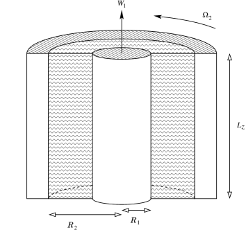
Figure 1: Geometrical configuration of the simulations. The outer cylinder rotates at angular velocity $\Omega_{2}$, while the inner cylinder moves in the axial direction at speed $W_{1}$.

In the absence of a magnetic field, viscosity causes the fluid between the cylinders to adjust itself to the spiral Couette velocity profile

$$\Omega^{\rm(C)}=C_{1}\biggl{(}1-\frac{R_{1}^{2}}{r^{2}}\biggr{)},\qquad u_{z}^{\rm(C)}=C_{2}\ln\frac{R_{2}}{r},$$ (7)

where

$$C_{1}=\frac{\Omega_{2}R_{2}^{2}}{R_{2}^{2}{-}R_{1}^{2}},\qquad C_{2}=\frac{W_{1}}{\ln(R_{2}/R_{1})}.$$

The velocity profile (7), driven by the viscous stress, adjusts itself over the viscous relaxation time,

$$\tau_{\rm visc}\approx\frac{(R_{2}{-}R_{1})^{2}}{\pi^{2}\nu}.$$ (8)

Table 1: Parameters of the numerical simulations discussed in the text. For all runs, $R_{1}=0.3$, $R_{2}=1.2$, $L_{z}=4$, $\Omega_{1}=0$, and $W_{2}=0$. The values of $W_{1}$, $\Omega_{2}$, $\nu$ and $\eta$ different from those of Model 1a are highlighted with bold face. The mesh has equal spacings in all three dimensions, $\delta x=\delta y=\delta z$ in all models except Model 1i where $\delta y=\delta x=\delta z/2$. Lengths are measured in units of $R_{0}$, angular velocities in $\Omega_{0}$, viscosity and diffusivity in $R_{0}^{2}\Omega_{0}$ and velocities in $R_{0}\Omega_{0}$.

Model	$W_{1}$	$\Omega_{2}$	$\nu$	$\eta$	$U$	$U_{\rm max}$	${\rm Re}$	${R}_{\rm m}$	${P}_{\rm m}$	$\delta x$
1a	$1.0$	$1.3$	$2\,{\times}\,10^{-2}$	$7\,{\times}\,10^{-3}$	$1.85$	$1.56$	$111$	$318$	$\phantom{0}2.9$	$0.033$
1b	$1.0$	$1.3$	$7\,{\times}\,10^{-2}$	$7\,{\times}\,10^{-3}$	$1.85$	$1.55$	$31.8$	$318$	$10$	$0.067$
1c	$1.0$	$1.3$	$1\,{\times}\,10^{-2}$	$7\,{\times}\,10^{-3}$	$1.85$	$1.55$	$222$	$318$	$\phantom{0}1.4$	$0.067$
1d	$1.0$	$1.3$	$2.5\,{\times}\,10^{-3}$	$7\,{\times}\,10^{-3}$	$1.85$	$1.55$	$889$	$318$	$\phantom{0}3.6$	$0.033$
1e	$1.0$	$1.3$	$1\,{\times}\,10^{-3}$	$7\,{\times}\,10^{-3}$	$1.85$	$1.55$	$2220$	$318$	$\phantom{0}0.14$	$0.017$
1f	$1.0$	$1.3$	$2\,{\times}\,10^{-2}$	$8\,{\times}\,10^{-3}$	$1.85$	$1.55$	$111$	$278$	$\phantom{0}2.5$	$0.067$
1g	$1.0$	$1.3$	$2\,{\times}\,10^{-2}$	$4\,{\times}\,10^{-3}$	$1.85$	$1.55$	$111$	$555$	$\phantom{0}5.0$	$0.067$
1h	$1.0$	$1.3$	$2\,{\times}\,10^{-2}$	$2\,{\times}\,10^{-3}$	$1.85$	$1.56$	$111$	$1110$	$10$	$0.033$
1i	$1.0$	$1.3$	$2\,{\times}\,10^{-2}$	$1\,{\times}\,10^{-3}$	$1.85$	$1.56$	$111$	$2220$	$20$	$0.017$
2a	$0.5$	$1.3$	$2\,{\times}\,10^{-2}$	$4\,{\times}\,10^{-3}$	$1.64$	$1.55$	$98$	$491$	$\phantom{0}5.0$	$0.033$
2b	$0.5$	$1.3$	$1\,{\times}\,10^{-2}$	$4\,{\times}\,10^{-3}$	$1.64$	$1.55$	$197$	$491$	$\phantom{0}2.5$	$0.067$
2c	$0.5$	$1.3$	$7\,{\times}\,10^{-2}$	$4\,{\times}\,10^{-3}$	$1.64$	$1.55$	$197$	$491$	$18$	$0.067$
2d	$0.5$	$1.3$	$2\,{\times}\,10^{-2}$	$2\,{\times}\,10^{-3}$	$1.64$	$1.55$	$98$	$984$	$10$	$0.033$

III.2 Basic equations

The equations we solve are the MHD equations for the vector potential ${\bf A}$, the velocity ${\bf u}$ and the density $\varrho$:

$$\frac{\partial{\bf A}}{\partial t} = {\bf u}\,{\times}{\bf B}+\eta\Delta{\bf A}+(\nabla\cdot{\bf A})\nabla\eta,$$ (9)

$$\frac{D{\bf u}}{Dt} = -\frac{1}{\varrho}\nabla p+\frac{\mu}{\varrho}\left(\Delta{\bf u}+{\textstyle\frac{1}{3}}\nabla\nabla\cdot{\bf u}\right)+\frac{\bf j{\times}{\bf B}}{\varrho},$$ (10)

$$\ \frac{D\varrho}{Dt} = -\varrho\nabla\cdot{\bf u},$$ (11)

complemented by an isothermal equation of state, $p=c_{\rm s}^{2}\varrho$, with constant speed of sound $c_{\rm s}$. Here, the magnetic flux density ${\bf B}$ and electric current density $\bf j$ are given by ${\bf B}=\nabla\times{\bf A}$, $\mu_{0}\bf j=\nabla\times{\bf B}$; we denote with $D/Dt\equiv\partial/\partial t+({\bf u}\cdot\nabla)$ the advective derivative; $\mu$ is the dynamical viscosity (assumed constant). Below we refer to the Reynolds number based on the average kinematic viscosity, $\nu=\mu/\overline{\varrho}$.

Equation (9) implies the gauge

$$\eta\nabla\cdot{\bf A}+\Phi=0,$$ (12)

where $\Phi$ is the electrostatic potential, related to the electric field ${\bf E}$ by ${\bf E}=-\nabla\Phi-\partial{\bf A}/\partial t$. This gauge proved to be most convenient for numerical purposes. Equations (9)–(11) are written for compressible fluids, but our choice of parameters makes compressibility insignificant since the speed of sound is a factor of two larger than the maximum fluid velocity, which results in a density contrast of $\leq 12\%$.

We use an explicit finite-difference scheme of sixth order in space and third order in time described, e.g., in Ref. (Sánchez-Salcedo and Brandenburg, 2001). The velocity field outside the fluid shell, i.e. for $r<R_{1}$ and $r>R_{2}$, is prescribed and fixed, with ${\bf u}=(0,0,W_{1})$ in $r<R_{1}$ and ${\bf u}=(0,\Omega_{2}r,0)$ in $r>R_{2}$. We embed the cylinders into a Cartesian box and solve Eqs. (9)–(11) on a Cartesian mesh in order to avoid a coordinate singularity on the axis and to retain the applicability of the code to different geometries.

The magnetic diffusivity $\eta$ is assumed to be constant for $r<R_{2}-3\delta x$ (with $\delta x$ the mesh size), i.e. the inner cylinder has the same electric conductivity as the fluid, but $\eta$ smoothly decreases to zero in $R_{2}-3\delta x<r<R_{2}$. Thus, the last term in Eq. (9) is only relevant close to the outer boundary of the fluid. The outer cylinder is assumed to be magnetically impenetrable, which confines the magnetic field to the region $r<R_{2}$. This would best be achieved with a perfect conductor at $r\geq R_{2}$, but this corresponds to an infinite magnetic Reynolds number, the numerical implementation of which leads to fundamental difficulties. Therefore we use the stronger requirement ${\bf A}={\bf 0}\text{ for }r\geq R_{2}$ instead. We demonstrate in Sect. IV.1 that our results are consistent with those obtained with a perfectly conducting outer cylinder since the magnetic field tends to concentrate close to the inner radius $R_{1}$ and thus the outer boundary condition only weakly affects the solution. We have counter-checked our results with a modified magnetic condition, where the vector potential is ‘softly’ set to zero in the region $r>R_{2}$ by means of an additional relaxation term $-{\bf A}/\tau_{{\bf A}}$ in the induction equation (9), and we only report results that are not qualitatively affected by this change.

In all three directions, periodic boundary conditions are assumed, which are imposed on the faces of the computational box. The horizontal boundary conditions are not actually important, since both the fluid and the magnetic field are confined to $r<R_{2}$. In the axial direction (the $z$-direction), the assumption of periodicity introduces a maximum wavelength $L_{z}$ (the vertical size of the box) and leads to a quantization of the vertical wavenumber $k$ to

$$k_{n}=2\pi n/L_{z},$$ (13)

with integer $n$, for solutions that are harmonic in $z$. To assess the role of this quantization, we have carried out one numerical experiment with a four times larger length $L_{z}=16$, which introduces additional modes, which can have values of $k$ four times closer to each other. The result was qualitatively quite similar to our other models. The only significant difference was that the system now had two modes with different $k$, but very similar growth rates, which introduced a relatively slow drift of energy from one mode to the other. We will not discuss this simulation in the following, but rather focus on the case of one fixed value of $L_{z}$ to ensure the comparability of the different models.

Figure 2 shows how the quantization of $k$ due to the finite value of $L_{z}$ affects the dynamo system. We show the dependence of the kinematic growth rate $\gamma$ on the continuous wave number $k$ — obtained by solving the eigenvalue problem (20)–(21) as described in Sect. IV.1 — and indicate the quantized values $k_{n}$ which occur in our simulations. While the maximum growth rate can be up to 40% larger than the maximum rate measured at $k_{n}$ (Model 1d), the optimal values of $k$ do not differ much from $k_{1}$. Thus, our choice of $L_{z}$ does not impose unrealistically small vertical scales on the magnetic field.

III.3 Parameters

The dynamo and hydrodynamical properties of the system are characterized by two non-dimensional quantities, the kinematic and magnetic Reynolds numbers, which are defined as

$${\rm Re}={UR_{2}}/{\nu},\qquad{R}_{\rm m}={UR_{2}}/{\eta},$$ (14)

where $U=\sqrt{(R_{2}\Omega_{2})^{2}{+}W_{1}^{2}}$ is a characteristic velocity. The ratio of the two Reynolds numbers is the magnetic Prandtl number

$${P}_{\rm m}={R}_{\rm m}/{\rm Re}.$$ (15)

We introduce a reference radius $R_{0}$ and a reference angular velocity $\Omega_{0}$ such that $R_{2}=1.2R_{0}$ and $\Omega_{2}=1.3\Omega_{0}$, i.e. the radial extent of the system and the revolution time are of order unity when measured in units of $R_{0}$ and $\Omega_{0}$, respectively. In the following, we will measure length in units of $R_{0}$, time in units of $1/\Omega_{0}$ and velocity in units of $R_{0}\Omega_{0}$, without explicitly indicating this in the text.

The parameter range investigated here is indicated in Table 1. Parameters that remain constant for all the simulations are the cylinder radii ($R_{1}=0.3$ and $R_{2}=1.2$), and the size of the computational box: $L_{z}=4$ for the vertical size and $L_{x}=L_{y}=2(R_{2}+3\delta x)$ for the horizontal dimensions. The numerical resolution is either $42{\times}42{\times}60$ (corresponding to $\delta x\approx 0.067$) or $78{\times}78{\times}120$ grid points ($\delta x\approx 0.033$) except for Model 1i where the higher resolution of $144\times 144\times 120$ ($\delta x\approx 0.017$) was used.

Figure 2: Kinematic growth rate $\gamma$ versus vertical wave number $k$ for Models 1f ($\cdots$), 1a ( ), 1g ($-\,-$), 1h ($-\cdot-\cdot{}$). and 1i ($-\cdot\cdot\cdot-\cdot\cdot\cdot{}$). The first two wave numbers $k_{1}$, $k_{2}$ allowed by $L_{z}=4$ are indicated by vertical arrows.

For the parameters used, the viscous relaxation time (8) is in the range 1–80 for the models discussed below. For comparison, the growth time of the magnetic field is greater than about 43 for the models presented, and the turnover time is $2\pi/|\Omega_{2}{-}\Omega_{1}|\approx 4.8$.

Models 1 and 2 differ in the value of $W_{1}$ and have therefore different velocity profiles. This results in different dynamo efficiencies; for example, ${R}_{\rm m}^{\rm(cr)}=218$ in Model 1 and ${R}_{\rm m}^{\rm(cr)}=384$ in Model 2. Another important distinction is the position of the magnetic field maximum, $r_{0}$: in Model 1, the magnetic field is localized closer to the inner cylinder than in Model 2 (see e.g. the insets in Figs. 3 and 4 or Fig. 12 in Appendix B). The models are further subdivided (1a–f, 2a–d) according to the values of $\nu$ and $\eta$ in order to explore the effects of varying magnetic and kinematic Reynolds numbers. Most of our models have ${P}_{\rm m}>1$, except Model 1d (${P}_{\rm m}\approx 0.36$) and Model 1e (${P}_{\rm m}=0.14$).

Figure 3: Kinematic growth rate $\gamma$ and frequency $\omega$ in Model 1 for the mode $m=1$, $k=k_{1}$ (the dominant mode) as a function of the magnetic Reynolds number, obtained from the one-dimensional eigenvalue problem described in Sect. IV.1. Dotted lines show the dependencies $\gamma\propto{R}_{\rm m}^{-1/3}$ and $\gamma\propto{R}_{\rm m}^{-1/2}$ in the upper panel and $(\omega-\mbox{const})\propto{R}_{\rm m}^{-1/2}$ in the lower panel. The asymptotic solution given in Appendix A is shown dashed. Results from the three-dimensional simulations are labeled according to the grid spacing: $\delta x=0.13$ ($+$), $0.067$ ($\diamond$), $0.033$ ($\Box$), and $0.017$ ($*$). The insets show radial magnetic energy profiles in the domain $0<r<R_{2}$ for ${R}_{\rm m}=2\,{\times}\,10^{3}$ (top) and ${R}_{\rm m}=2\,{\times}\,10^{5}$ (bottom); the region occupied by the inner cylinder is shaded. The generation threshold for this configuration is ${R}_{\rm m}^{\rm(cr)}\approx 218$.

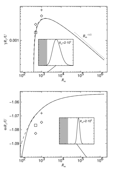
Figure 4: As in Fig. 3, but for Model 2. The critical magnetic Reynolds number is ${R}_{\rm m}^{\rm(cr)}\approx 384$.

IV Results

IV.1 Kinematic regime

The velocity profile (7) can be considered as fixed, and Eq. (2) as linear in ${\bf B}$, as long as the magnetic stress is weak compared to the viscous stress,

$$\frac{B^{2}}{\mu_{0}}\ll\varrho\nu\frac{U}{R_{2}{-}R_{1}}.$$ (16)

Equations for the resulting kinematic dynamo problem are given in Appendix A. As discussed in Sect. II, they represent a one-dimensional eigenvalue problem which is relatively straightforward to solve numerically. For Models 1 and 2 we show in Figs. 3 and 4 the dependence of the growth rate $\gamma$ and frequency $\omega$ on the magnetic Reynolds number (solid lines) and compare them to the asymptotic formulae, which are given in Ref. Ruzmaikin et al. (1989) and are also reproduced in Appendix A (dashed lines in Figs. 3 and 4). The insets show the radial profile of magnetic energy for two values of ${R}_{\rm m}$.

The growth rate $\gamma$ becomes positive at ${R}_{\rm m}={R}_{\rm m}^{\rm(cr)}$, first quickly increases with ${R}_{\rm m}$, and then decreases as expected for a slow dynamo Zeldovich et al. (1983); Soward (1990). For the continuous velocity profile (7), the analytic theory predicts an asymptotic decrease $\gamma\propto{R}_{\rm m}^{-1/2}$ (Appendix A), and this scaling is indeed reached for very large values of ${R}_{\rm m}$. However, while the growth rate for Model 2 (Fig. 4) agrees well with the asymptotic result (dashed), the agreement is not so good for ${R}_{\rm m}\lesssim 2000$ in Model 1 (Fig. 3). Moreover, the latter model shows a transient approximate scaling $\gamma\sim{R}_{\rm m}^{-1/3}$. Incidentally, this scaling is close to that for a flow with discontinuous radial profile Ponomarenko (1973); Gilbert (1988a).

The difference can be explained as follows. For moderate magnetic Reynolds numbers, the field has noticeable strength at the boundary of the inner cylinder in the flow of Model 1 (see inset in the top frame of Fig. 3). Therefore, the asymptotic theory is inapplicable as it is based on the assumption that the magnetic field is concentrated far from the boundaries $r=R_{1}$ and $r=R_{2}$. However, the radial width of the field distribution decreases with ${R}_{\rm m}$ and eventually the field at $r=R_{1}$ becomes negligible (see inset in the bottom frame of Fig. 3), and the scaling $\gamma\sim{R}_{\rm m}^{-1/2}$ is recovered. On the other hand, the field is always small near the boundaries in Model 2 (see insets in Fig. 4), and so the scaling $\gamma\sim{R}_{\rm m}^{-1/3}$ does not occur.

We have also explored the linear stage of magnetic field evolution using the three-dimensional code in order to assess its performance. A discussion of the numerical aspects is given in Appendix B. We initialize the simulations with a weak random magnetic field. After the initial transients have died away, exponential growth of magnetic energy is established, corresponding to the fastest growing mode.

Figure 5a shows the magnetic field structure for Model 1h. The level surfaces of $|{\bf B}|$ have the form of two helical flux tubes of opposite field orientation, which corresponds to an azimuthal wavenumber $m=1$. The vertical wavenumber of the solution shown is $k=2\pi/L_{z}=\pi/2$. This mode is excited in all the models of Table 1. However, additional higher modes are excited in Models 1h, 1i, and 2d, where ${R}_{\rm m}$ is larger (see Table 2).

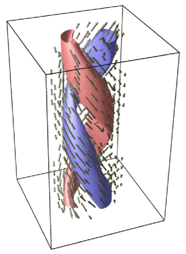
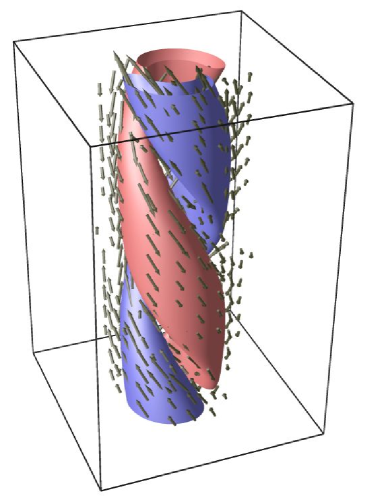
 (a)  (b)

Figure 5: Three-dimensional representation of the magnetic field in Model 1h. (a) $t=200$ (end of the kinematic stage); (b) $t=912$ (the saturated state). Shown are surfaces where $|{\bf B}|$ is 0.65 of the maximum and magnetic field vectors. The vertical component of the field has opposite sign in the two flux tubes shown (mode $m=1$). The azimuthal and axial variations of the field are harmonic at the kinematic stage (a) and flattened in the saturated state (b) (see also Fig. 6).

Both the flow and the magnetic field are strongly helical, the two helicities being of opposite sign (the streamlines are right-handed spirals, while the magnetic field lines form left-handed helices as can be seen in Fig. 5). Since the screw dynamo mechanism relies on diffusion, the approximate conservation of magnetic helicity in highly conducting media, which leads to serious difficulties in mean-field dynamo theory Blackman and Field (1999); Brandenburg (2001), does not lead to any problem here.

IV.2 Nonlinear Simulations

After a phase of exponential growth, magnetic energy levels off at a certain saturation value. The corresponding magnetic energy density is comparable to (but smaller than) the kinetic energy density in the sheared flow, as can be seen from Table 2, where we compare the maximum magnetic flux density to $\sqrt{\overline{\varrho}U^{2}}$, and the magnetic energy to $E_{\rm kin}=\frac{1}{2}\overline{\varrho}U^{2}V$, where $V=L_{z}\pi(R_{2}^{2}{-}R_{1}^{2})$ is the fluid volume. The location and width of the magnetic energy maximum are characterized by

$$r_{B}=\left<r\right>_{{\bf B}^{2}},\qquad\delta r_{B}=\left<(r{-}r_{B})^{2}\right>_{{\bf B}^{2}}^{1/2},$$ (17)

where $\left<f\right>_{{\bf B}^{2}}=\int f\,{\bf B}^{2}\,dV/\int{\bf B}^{2}\,dV$ is the magnetic-energy weighted volume average. These quantities are similar to $r_{0}$ and $\delta r$ of the kinematic theory.

Table 2: Magnetic field properties in the models of Table 1. Numbers in parentheses refer to the kinematic stage, all other quantities are for the saturated state. Shown are the growth rate $\gamma$ and oscillation frequency $\omega$ of the leading mode; the maximum saturated magnetic field strength $B_{\rm max}$ and magnetic energy $E_{\rm mag}$ in the flow region, both normalized to the corresponding kinetic quantities; and the position and width of the magnetic field distribution in radius, $r_{B}$ and $\delta r_{B}$. The last column lists the growing modes in the form $(m,kL_{z}/(2\pi))$, $L_{z}=4$, ordered by decreasing growth rate. The results for Models 1h, 1i, and 2d refer to the $(1,1)$ mode only. Growth rates and oscillation frequencies are measured in units of $\Omega_{0}$, lengths in $R_{0}$.

Model	$\gamma$	$\omega$		$\displaystyle\frac{B_{\rm max}}{\sqrt{\overline{\varrho}U^{2}}}$	$\displaystyle\frac{E_{\rm mag}}{E_{\rm kin}}$	$r_{B}$		$\delta r_{B}$		$(m,2k/\pi)$
1a	($0.0160$)	$-2.03\phantom{0}$	($-1.957$)	$0.33$	$0.015$	$0.49$	($0.47$)	$0.17$	($0.16$)	$(1,1)$
1b	($0.0144$)	$-2.014$	($-1.957$)	$0.51$	$0.034$	$0.48$	($0.47$)	$0.17$	($0.16$)	$(1,1)$
1c	($0.0144$)	$-2.037$	($-1.957$)	$0.24$	$0.008$	$0.48$	($0.47$)	$0.17$	($0.16$)	$(1,1)$
1d	($0.0144$)	$-2.045$	($-1.957$)	$0.14$	$0.002$	$0.50$	($0.47$)	$0.17$	($0.16$)	$(1,1)$
1e	($0.0144$)	$-2.051$	($-1.957$)	$0.08$	$0.0009$	$0.51$	($0.47$)	$0.17$	($0.17$)	$(1,1)$
1f	($0.0087$)	$-2.014$	($-1.976$)	$0.25$	$0.008$	$0.48$	($0.47$)	$0.17$	($0.17$)	$(1,1)$
1g	($0.0232$)	$-2.028$	($-1.935$)	$0.42$	$0.024$	$0.47$	($0.47$)	$0.15$	($0.14$)	$(1,1)$
1h	($0.0176$)	$-2.012$	($-1.91$)	$0.47$	$0.030$	$0.47$	($0.46$)	$0.13$	($0.12$)	$(1,1)$, $(1,2)$
1i	(—)	$-1.981$	(—)	$0.55$	$0.035$	$0.46$	(—)	$0.11$	(—)	$(1,2)$, $(1,1)$, $(2,3)$, $(2,1)$, $(2,2)$
2a	($0.0023$)	$-1.459$	($-1.471$)	$0.17$	$0.006$	$0.63$	($0.66$)	$0.18$	($0.18$)	$(1,1)$
2b	($0.0039$)	$-1.459$	($-1.473$)	$0.23$	$0.10$	$0.65$	($0.67$)	$0.21$	($0.20$)	$(1,1)$
2c	($0.0039$)	$-1.506$	($-1.488$)	$0.48$	$0.41$	$0.63$	($0.66$)	$0.20$	($0.20$)	$(1,1)$
2d	($0.0071$)	$-1.506$	($-1.467$)	$0.29$	$0.01$	$0.61$	($0.66$)	$0.17$	($0.17$)	$(1,1)$, $(1,2)$

IV.2.1 Spatial structure of the magnetic field

Figure 6 shows the vertical profiles of the magnetic field in the saturated regime for various magnetic Reynolds numbers. The vertical component of the magnetic field is plotted as a function of $z$ close to the radius where the field concentrates. Note that the antisymmetry of the curve with respect to the middle of the box indicates that only Fourier components with odd vertical wavenumbers are excited, which can be understood from the structure of the nonlinear terms in Eqs. (9)–(11). The profile in the saturated state is flattened in comparison to the (kinematic) eigenmode and this effect becomes more pronounced as ${R}_{\rm m}$ increases. The flattening of the maxima in both $z$ and $\varphi$ can also be seen in Fig. 5, where the level surface $|{\bf B}|=0.65\,|{\bf B}|_{\rm max}$ is shown toward the end of the linear phase (Fig. 5a) and in the saturated state (Fig. 5b).

The strongly anharmonic profiles $B(z)$ found for large ${R}_{\rm m}$ do not occur in Bassom and Gilbert’s Bassom and Gilbert (1997) theory, which predicts harmonic profiles in the saturated state. The difference may be due to the fact that here ${P}_{\rm m}>1$, whereas Bassom & Gilbert assume ${P}_{\rm m}\ll 1$. The sensitivity of the solution to the value of the magnetic Prandtl number (if this is the true reason for the difference) is striking.

As can be seen in Fig. 7, the nonlinear distortion of the magnetic field distribution is only prominent in the azimuthal and axial profiles, but not much in the radial profile. We also note from Table 2 that in all the models the radial width $\delta r_{B}$ of the magnetic energy distribution in the nonlinear stage is not significantly larger than that in the kinematic stage. In Model 1h, for example, the radial width of the eigenfunction is $\delta r_{B}\approx 0.12$ during the linear stage and $0.13$ at saturation. These numbers hardly differ and are very close to $\delta r$ from the asymptotic theory, which equals $\delta r=R_{2}{\cal O}({R}_{\rm m}^{-1/3})\simeq 0.11$ for a discontinuous velocity profile and $\delta r=R_{2}{\cal O}({R}_{\rm m}^{-1/4})\simeq 0.20$ for a smooth profile. In all our simulations, the radial width of the magnetic field distribution in both linear and nonlinear states are very close to each other and also close to that predicted by the asymptotic theory for the kinematic dynamo. This is at variance with the nonlinear asymptotics of Bassom and Gilbert (1997) that predict the development of a ‘core’ region in the radial profile of magnetic field with a width of order ${\cal O}({R}_{\rm m}^{-1/10})\simeq 0.5$ in Model 1i. A possible reason for this discrepancy might be that our models have too small values of ${R}_{\rm m}$ (2220 in Model 1i and 984 in Model 2d) for the asymptotic regime of Bassom & Gilbert to apply, even though the linear asymptotics are already accurate. It is more plausible, however, that solutions with moderate magnetic Prandtl number do not develop the ${R}_{\rm m}^{-1/10}$ core and their radial profile is quite similar to that of the kinematic eigenfunction (see Fig. 7).

Figure 6: Magnetic field structure in the saturation regime. Shown is, as a function of $z$, the vertical field $B_{z}$ along a vertical line at $r=0.48$ for Models 1f, 1a, 1g, 1h, and 1i; ${R}_{\rm m}$ grows monotonically along this sequence.

Figure 7: Radial magnetic field profile in the saturated regime for Models 1i (top; ${P}_{\rm m}=20$), and 1e (bottom; ${P}_{\rm m}=0.14$). Shown is the vertically averaged magnetic energy density as a function of $r$ (dots) and the corresponding profile at the kinematic dynamo stage (dashed). The maximum of $\left<{\bf B}^{2}\right>_{z}$ is normalized to one; radius is measured in units of $R_{0}$.

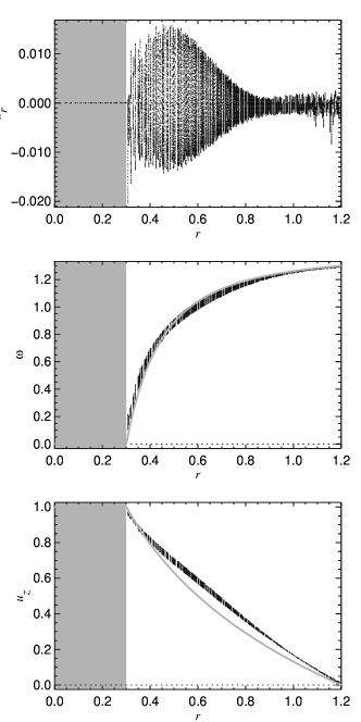
Figure 8: Radial, azimuthal and vertical velocity components as functions of radius in the saturated stage for Model 1a at a resolution $\delta x=0.033$. Note the different ranges on the ordinate in the panels: the variation of $u_{r}$ is much smaller than that of $u_{\varphi}$ or $u_{z}$. The shear in both $\omega(r)$ and $u_{z}(r)$ is reduced in comparison to that in the Couette profile ${\bf u}^{\rm(C)}$ of Eq. (7), which is shown as a continuous gray line. The location of the inner cylinder is marked in gray. The scatter of the data points arises from their different positions in $\varphi$ and $z$. Velocities are measured in units of $R_{0}\Omega_{0}$, angular velocities in units of $\Omega_{0}$ and radius in units of $R_{0}$. (In units of $U$ and $R_{2}$, the value $u_{r}=0.01$ corresponds to $0.0054U$, and $\omega=1.2$ corresponds to $0.78U/R_{2}$, for example.)

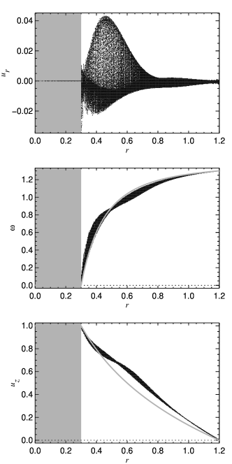
Figure 9: As Fig. 8, but for Model 1i.

IV.2.2 Nonlinear distortion of the velocity field

Figure 8 shows the radial velocity profiles for the saturated phase of Model 1a where the scatter of the data points is due to their different positions in $\varphi$ and $z$. The radial velocity fluctuates around zero and is dynamically unimportant (even more so as perturbations in the radial velocity can be balanced by the pressure gradient). However, the azimuthal and axial velocities exhibit systematic deviations from their Couette profiles so that the velocity shear is reduced in the region where the magnetic field concentrates. It is especially clear in the case of $u_{z}$ (Fig. 8c) that the spatial scatter is smaller than the mean variation, so the distortion of the velocity field is axially symmetric and independent of $z$ to a first approximation. To justify this we demonstrate in Fig. 10 that the radial profiles of the averaged Lorentz force are in close correspondence with the deviations of the respective velocity components of Fig. 8 from the Couette profile. This is compatible with the scenario of Bassom and Gilbert (1997), where, in the limit of infinite kinematic and magnetic Reynolds numbers, the saturation of dynamo action is mainly due to the vertically and azimuthally averaged part of the Lorentz force. As the magnetic Reynolds number is increased, the relative distortion of the velocity field, and in particular the reduction of velocity shear, are getting more pronounced; this can be seen in Fig. 9, where we show the same profiles as in Fig. 8, but for a seven times larger value of ${R}_{\rm m}$.

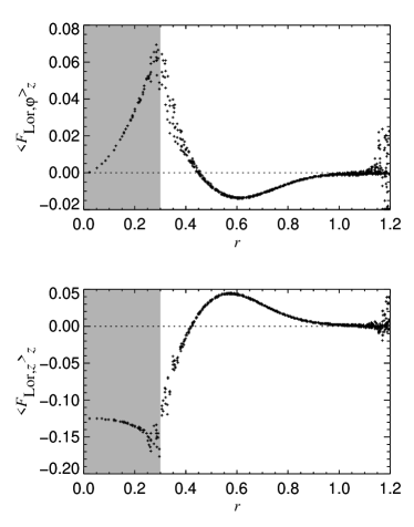
Figure 10: Vertically averaged components of the Lorentz acceleration ${\bf F}_{\rm L}=\bf j\times{\bf B}/\varrho$ as a function of radius for Model 1a. Note that the effects of magnetic torques on the inner cylinder (shaded area in Fig. 10) are ignored in our model and its velocity remains fixed. Velocities are measured in units of $R_{0}\Omega_{0}$, angular velocities in units of $\Omega_{0}$ and radius in units of $R_{0}$. ${\bf F}_{\rm L}$ is measured in units of $R_{0}\Omega_{0}^{2}$, radius in units of $R_{0}$. (In units of $U$ and $R_{2}$, the value $F_{\rm Lor}=0.05$ corresponds to $0.018U^{2}/R_{2}$, for example.)

The radial width of the region where the velocity field is distorted away from the original Couette profile is much larger than that of the Lorentz force (see Fig. 10 below). This happens because the flow adjusts itself to two separate Couette profiles at both ends of the radial range where the Lorentz force has distorted it, and so a localized magnetic field does affect the flow throughout the domain. It can be expected that a flow profile driven by a volume force will be distorted less in regions where magnetic field is weak; our results confirm this expectation.

The screw dynamo can be interpreted in terms of the mean-field $\alpha\Omega$-dynamo Soward (1990); Gilbert and Ponty (2000), the $\Omega$-term being as usual the shear term $rB_{r}\,d\Omega/dr$ [see Eq. (21)]. The $\alpha$-effect is identified with a part of the diffusion term, and the corresponding term in the induction equation has the form

$$-\eta\frac{2}{r^{2}}\frac{\partial}{\partial\varphi}B_{\varphi}$$ (18)

[see also Eq. (20)]. Since the differential operator acting on $B_{\varphi}$ is obviously not influenced by the magnetic field strength, the $\alpha$-effect cannot be affected by the growing magnetic field and saturation is fully due to $\Omega$-quenching. This is opposite to one of the standard scenarios for mean-field dynamos ($\alpha$-quenching), where the magnetic field has little influence on the angular velocity and saturation is considered to be caused by the partial suppression of the $\alpha$-effect by magnetic fields.

Figure 11: Magnetic energy in the saturated state versus the kinematic and magnetic Reynolds numbers for Models 1a–i. Top: $E_{\rm mag}/E_{\rm kin}$ as a function of ${\rm Re}$ for Models 1b, 1a, 1c, 1d, and 1e (asterisks). The crosses refer to a model with volume forcing (see Sect. IV.2.3). Bottom: $E_{\rm mag}/E_{\rm kin}$ as a function of ${R}_{\rm m}$ for Models 1f, 1a, 1g, 1h, and 1i. The dashed lines show the asymptotic power laws given in Eq. (6); the dotted line is a least-square power-law fit and corresponds to a dependence $E_{\rm mag}\propto{\rm Re}^{-0.84}$.

IV.2.3 Scaling of magnetic energy with ${\rm Re}$ and ${R}_{\rm m}$

Figure 11 shows the magnetic energy in the saturated state as a function of the kinematic and magnetic Reynolds numbers. We also show the asymptotic scalings of Bassom and Gilbert (1997). There is clearly some agreement between the numerical and asymptotic results although the asymptotic solution has been obtained for ${P}_{\rm m}\ll 1$ whereas the numerical results refer mostly to the case ${P}_{\rm m}>1$. We believe that the reason for the rough agreement is related to the fact that, in both cases, the magnetic feedback affects mainly the axisymmetric flow profile, as was seen in Fig. 8.

As expected (at least for weakly supercritical solutions) the steady-state magnetic field strength $B_{\rm ss}$ increases with magnetic Reynolds number. On the other hand, the saturated field strength $B_{\rm ss}$ decreases with ${\rm Re}$ in a flow driven by viscous stresses because it becomes easier for the magnetic field to modify the velocity field in a given cylindrical shell as ${\rm Re}$ increases (owing to the weaker viscous coupling of fluid at different radii), and so a weaker magnetic field is needed to achieve a local reduction in shear sufficient to halt the field growth. As we discuss below, this behavior is characteristic of a flow driven by viscous stresses rather than by a volume force.

The scaling of magnetic energy with ${\rm Re}$ is slightly shallower than predicted by Bassom & Gilbert and has an exponent close to $-0.84$ rather than $-1$. Similarly, the growth of magnetic energy with ${R}_{\rm m}$ is slower than ${R}_{\rm m}^{2/5}$ at the values of ${R}_{\rm m}$ explored here. The most plausible reason for these disagreements is the difference in magnetic Prandtl numbers and, possibly, also the fact that the magnetic field distribution is still not narrow compared to the gap width $R_{2}{-}R_{1}$ for the magnetic Reynolds numbers we were able to consider.

Taken at face value, the dependence of $B_{\rm ss}$ on ${\rm Re}$ discussed above implies that the resulting magnetic field will be negligible wherever ${\rm Re}\gg 1$. However, in most real systems the flow will be driven by non-viscous forces. These are pressure and inertial forces in the dynamo experiments in Riga and Perm. In the case of astrophysical jets, acceleration and collimation of the flow can be due to an external magnetic field (axisymmetric to the first approximation, then the screw dynamo can generate an additional nonaxisymmetric magnetic field). In these cases the kinematic Reynolds number will not play such a prominent role in the system and $B_{\rm ss}$ is expected to be independent of ${\rm Re}$ for ${\rm Re}\gg 1$.

To verify this idea, we have carried out further numerical simulations for the parameters of Models 1b, 1a, 1c, and 1d, but with an additional volume force

$$-\frac{{\bf u}{-}{\bf u}^{\rm(C)}}{\tau}$$ (19)

on the right-hand side of the equation of motion (10). Here ${\bf u}^{\rm(C)}$ denotes the spiral Couette profile (7) and $\tau$ is the time scale over which the flow adjusts itself to the Couette profile. With our choice $\tau=1$, we have $\tau\lesssim\tau_{\rm visc}$, where the viscous time $\tau_{\rm visc}$ varies in the range 1–80, cf. Eq. (8). Thus, the Couette flow profile is now maintained on a dynamical time scale rather than by viscosity if ${\rm Re}\gg 30$.

We show in Fig. 11 by crosses the resulting dependence of the steady-state magnetic energy on ${\rm Re}$; the dependence is clearly much weaker than in the case of viscous driving (a power-law fit to the points shown has an exponent of about $-0.41$). In the inviscid limit ${\rm Re}\to\infty$ the magnetic energy must eventually become independent of viscosity, and so we anticipate that the dependence marked with crosses has a horizontal asymptote.

Another reason why the dependence (6) is not directly applicable to laboratory and astrophysical dynamos is that the corresponding flows are turbulent. In that case the generation of magnetic field on the scale of the mean flow can be accompanied by the so-called ‘fluctuation dynamo’ producing small-scale magnetic fields, which eventually achieves energy equipartition with the turbulence. For small magnetic Prandtl number, however, the dynamo is only weakly supercritical and only large scales can be excited. Thus, the screw dynamo effect is expected to work, but it is now controlled by the effective values of ${\rm Re}$ and ${R}_{\rm m}$ based on turbulent diffusivities. We conjecture that this could still be qualitatively true in the nonlinear phase of field evolution. Since the turbulent values of ${\rm Re}$ and ${R}_{\rm m}$ can be quite moderate, even the scaling (6) would not lead to physically uninteresting magnetic fields. It can be expected, however, that the turbulence in the Couette flow — being generated mainly in turbulent boundary layers near the flow boundaries — will be very inhomogeneous and this can affect the theory discussed here. On the other hand, the reduction in the effective magnetic Reynolds number due to turbulence has to be only moderate since one needs ${R}_{\rm m}\geq{R}_{\rm m}^{\rm(cr)}$ for any sort of dynamo action. Assuming that turbulent magnetic and kinetic Reynolds numbers have similar orders of magnitude, ${\rm Re}\simeq{R}_{\rm m}$, and that ${R}_{\rm m}^{\rm(cr)}\simeq 10^{2}$, the resulting magnetic energy density will be about 10% of the kinetic energy density even with the scaling (6).

We note in this connection that the maximum radial magnetic field component measured in the Riga dynamo experiment (Gailitis et al., 2001) is about $6\,{\rm mT}$, while the equipartition field strength would be $\approx 0.5\,{\rm T}$. $B_{\varphi}$ and $B_{z}$ being about five times larger than $B_{r}$ in the kinematic case [F. Stefani, private communication], one gets a ratio $E_{\rm mag}/E_{\rm kin}\approx 5\,{\times}\,10^{-3}$. This is two orders of magnitude larger than ${R}_{\rm m}^{2/5}{\rm Re}^{-1}\lesssim 10^{-5}$ and clearly implies that the scaling (6), which is based on the assumption of a viscously driven, laminar flow, cannot be directly applied to flows in laboratory experiments.

All our experiments were carried out for angular velocity $\Omega$ increasing outwards and, for the boundary conditions and parameters considered, the flow was found to be hydrodynamically stable in the sense that the Lorentz force led to relatively small deviations from the unperturbed Couette profile (7). An interesting question is that of dynamo action in a spiral Couette flow unstable with respect to the magneto-rotational instability, i.e. for angular velocity decreasing outwards. Flows of this type — although for vanishing vertical velocities of the two cylinders — are currently discussed in connection with experimental investigations of the magneto-rotational instability Ji et al. (2001); Goodman and Ji (2002); Rüdiger and Zhang (2001). If the flow is hydrodynamically stable (angular momentum increasing outwards), a certain magnetic field is necessary to obtain regular Taylor columns; however, these columns involve a helical velocity field and are themselves capable of dynamo action Rüdiger and Zhang (2001). Thus, the magnetic field can play the role of a ‘catalyst’, destabilizing the system and at the same time regenerating it by the resulting instability; this mechanism has been demonstrated to occur in accretion discs Brandenburg et al. (1995); Balbus and Hawley (1998).

V Conclusions

The numerical calculations performed here have revealed a new intermediate asymptotic regime in the kinematic screw dynamo where, in a certain range of ${R}_{\rm m}$, the magnetic field eigenfunction is large enough at the flow boundary so that the standard asymptotic solutions are inapplicable and the growth rate of the magnetic field scales as $\gamma={\cal O}({R}_{\rm m}^{-1/3})$. This dependence is typical of a discontinuous velocity profile. The standard asymptotic scaling, $\gamma={\cal O}({R}_{\rm m}^{-1/2})$, is only recovered at significantly larger values of ${R}_{\rm m}$ where the eigenfunction becomes narrow enough in radius as to satisfy the assumptions of the asymptotic theory.

We have confirmed the result of Bassom and Gilbert (1997) that saturation of screw dynamo action occurs via a reduction in the velocity shear produced by the axisymmetric part of the Lorentz force. We have shown that this also applies to the case of large magnetic Prandtl numbers ${P}_{\rm m}$. However, the radial profile of the nonlinear solution is very similar to the marginally stable eigenmode for the nonlinearly modified velocity field. This is different from the nonlinear asymptotics of Bassom and Gilbert, which predicts a plateau in the radial dependence. It is possible that such a plateau can only occur at values of the magnetic Prandtl number much smaller than what we have been able to simulate in the present work, but we have not detected any tendency towards its development at ${P}_{\rm m}=0.14$, the smallest value explored here.

We have demonstrated that the scaling of the steady-state magnetic field with kinematic Reynolds number is sensitive to the nature of the forces driving the flow.

Appendix A One-dimensional kinematic dynamo problem

In cylindrical coordinates $(r,\varphi,z)$, the kinematic dynamo problem for given steady velocity field $\bigl{(}0,r\Omega(r),u_{z}(r)\bigr{)}$, is given by the following non-dimensionalized set of equations for the two amplitudes $\widehat{B}_{r}$, $\widehat{B}_{\varphi}$ [cf. Eq. (3)]:

$$\lambda\widehat{B}_{r}+{\rm i}(m\Omega{+}ku_{z})\widehat{B}_{r} = \frac{1}{{R}_{\rm m}}\left\{\hat{D}\widehat{B}_{r}-\frac{2{\rm i}m}{r^{2}}\widehat{B}_{\varphi}\right\},$$ (20)

$$\lambda\widehat{B}_{\varphi}+{\rm i}(m\Omega{+}ku_{z})\widehat{B}_{\varphi} = r\frac{d\Omega}{dr}\widehat{B}_{r}$$ (21)

$$\mbox{}\!+\frac{1}{{R}_{\rm m}}\left\{\hat{D}\widehat{B}_{\varphi}+\frac{2{\rm i}m}{r^{2}}\widehat{B}_{r}\right\}\!\!,\qquad$$

where

$$\hat{D} = \frac{1}{r}\frac{d}{dr}\left(r\frac{d}{dr}\right)-\frac{m^{2}{+}1}{r^{2}}-k^{2}$$ (22)

is a self-adjoint, Laplace-type differential operator, and $\lambda$ is the eigenvalue. The vertical component $B_{z}$ can be obtained from the solenoidality condition,

$$\frac{1}{r}\frac{d}{dr}(r\widehat{B}_{r})+\frac{{\rm i}m}{r}\widehat{B}_{\varphi}+{\rm i}k\widehat{B}_{z}=0.$$ (23)

Second-order asymptotic analysis (for ${R}_{\rm m}\to\infty$) for the spiral Couette flow (7) has been presented in Refs. Ruzmaikin et al. (1988, 1989). It is convenient to define the magnetic Reynolds number as

$$\widetilde{R}_{\rm m}=\frac{R_{1}^{2}R_{2}^{2}}{R_{2}^{2}{-}R_{1}^{2}}\frac{|\Delta\Omega|}{\eta}\equiv 2\frac{|\Omega^{\prime}(r)|r^{3}}{\eta}$$ (24)

here, which is different from the definition (14) used in the body of this paper. The radius $r_{0}$, where the magnetic field concentrates, is given by

$$r_{0}=R_{1}R_{2}\sqrt{\frac{\ln R_{2}{-}\ln R_{1}}{R_{2}^{2}{-}R_{1}^{2}}}\sqrt{-2\frac{m\Delta\Omega}{k\Delta W}}$$ (25)

and the field can only be growing if

$$\frac{m\Delta\Omega}{k\Delta W}<0,$$ (26)

where $\Delta\Omega=\Omega_{2}{-}\Omega_{1}$ and $\Delta W=W_{2}{-}W_{1}$.

To second order in the small parameter $\widetilde{R}_{\rm m}^{-1/2}$, the eigenvalue $\lambda$ of the fastest growing mode is given (in dimensional units) by

$$\lambda+{\rm i}[m\Omega(r_{0})+ku_{z}(r_{0})]$$ (27)

$$\quad= \frac{\eta}{r_{0}^{2}}\biggl{\{}(\sqrt{2}{-}1)\sqrt{|m|}(1{+}\sigma_{1}{\rm i})\widetilde{R}_{\rm m}^{1/2}$$

$$\qquad{}+\Bigl{(}\frac{17}{36}-\sqrt{2}-k^{2}r_{0}^{2}\Bigr{)}{}+{\cal O}\left(\widetilde{R}_{\rm m}^{-1/2}\right)\biggr{\}},\qquad$$

where $\sigma_{1}={\rm sgn}(k\Delta W)$ denotes the sign of $k\Delta W$. As $\eta\propto\widetilde{R}_{\rm m}^{-1}$, the leading-order term on the right-hand side is ${\cal O}\bigl{(}\widetilde{R}_{\rm m}^{-1/2}\bigr{)}$ when measured in the units $U/R_{2}$.

To the leading order in $\widetilde{R}_{\rm m}$, the magnetic field amplitudes $\widehat{B}$ are given by

$$\widehat{B}_{\varphi} = \exp\left[-(1{+}\sigma_{1}{\rm i})\sqrt{|m|\widetilde{R}_{\rm m}}\frac{(r{-}r_{0})^{2}}{2r_{0}^{2}}\right]$$ (28)

$${}+{\cal O}\left(\widetilde{R}_{\rm m}^{-1/2}\right),\qquad$$

$$\widehat{B}_{r} = \sigma_{2}(1{+}\sigma_{1}{\rm i})\sqrt{\frac{|m|}{2}}\widehat{B}_{\varphi}\widetilde{R}_{\rm m}^{-1/2}+{\cal O}\left(\widetilde{R}_{\rm m}^{-1}\right),$$ (29)

$$\widehat{B}_{z} = -\frac{m}{k}\left(\frac{1}{r}+\sqrt{2}\,\frac{r{-}r_{0}}{r_{0}^{2}}\right)\widehat{B}_{\varphi}+{\cal O}\!\left(\widetilde{R}_{\rm m}^{-1/2}\right)\!,\qquad$$ (30)

where $\sigma_{2}={\rm sgn}\,\Delta\Omega$.

Appendix B Accuracy of the numerical scheme

We assess the accuracy of our three-dimensional simulations and the implementation of the boundary conditions by comparing solutions obtained with the 3D code in the kinematic regime with those from the corresponding 1D eigenvalue problem.

The radial dependence of the (vertically averaged) magnetic energy density is shown in Fig. 12 for the high-resolution runs of Models 1a and 2a at a time when the exponential growth has well established itself. Magnetic energy concentrates in a cylindrical shell of radius $r_{B}$ and of half-width $\delta r_{B}$, defined in Eq. (17). For Model 1a (Fig. 12a), we find $r_{B}=0.48$ and $\delta r_{B}=0.16$ (see also Table 3). For comparison, we have overplotted the profile obtained from the one-dimensional model.

Figure 12: Radial field structure in the kinematic regime as obtained from a three-dimensional simulation at a resolution $\delta x=0.033$ (dots) and from solving the one-dimensional Eq. (20) with $R_{1}=0.28$ (solid). (a) Model 1a, (b) Model 2a. The maximum of $\left<{\bf B}^{2}\right>_{z}$ is normalized to one; radius is measured in units of $R_{0}$.

Figure 12 shows good agreement between the three-dimensional and one-dimensional simulations everywhere except close to the outer boundary. For $r\approx R_{2}$, the magnetic energy in the three-dimensional simulation smoothly turns to zero, while in the one-dimensional calculation the tangential components of ${\bf B}$ remain significant for Model 2a. This is due to the different boundary conditions used (${\bf A}={\bf 0}$ vs. perfectly conducting) and the close agreement of growth rates and eigenfunctions gives us reason to believe that these are not influenced by this localized deviation.

In Table 3, we compare the eigenvalues $\lambda$ and the spatial parameters $r_{B}$ and $\delta r_{B}$ of the magnetic field for the three-dimensional simulations with those from the one-dimensional model for different numerical resolutions. While the high-resolution simulation has only an error of about 5 % in the growth rate $\gamma$, and 0.3 % in the frequency $\omega$, the lower-resolution run yields errors of 18 % and 0.9 %, respectively. The main source of inaccuracy is the angular discretization of the inner cylinder boundary as illustrated in Fig. 13. If we define an effective inner radius $R_{1}^{\rm(eff)}$ as the radius of a circle enclosing the same area as the shaded cells in Fig. 13, then $R_{1}^{\rm(eff)}\approx 0.29$ for the lower-resolution run. For an inner radius of $0.29$, the one-dimensional model yields a growth rate that is considerably lower and closer to what is observed in the lower-resolution run (see Table 3). This adjustment of $R_{1}^{\rm(eff)}$ results in better agreement of $\omega,\ r_{B}$ and $\delta r_{B}$ as well.

Table 3: Accuracy of the three-dimensional code, illustrated for Model 1a using various resolutions $\delta x$. The effective inner radius $R_{1}^{\rm(eff)}$ is defined in the text. Growth rate, frequency, localization radius and width of the magnetic field distribution are given for Model 1a at different resolutions (top half). The lower half of the table shows the accurate values obtained by solving the one-dimensional problem (20), (21) for three different values of $R_{1}$. Lengths are measured in units of $R_{0}$, growth rates and oscillation frequencies in units of $\Omega_{0}$.

Model	$R_{1}^{\rm(eff)}$	$\gamma$	$\omega$	$r_{B}$	$\delta r_{B}$
1a ($\delta x{=}0.067$)	$0.291$	$0.0144$	$-1.969$	$0.467$	$0.162$
1a ($\delta x{=}0.033$)	$0.301$	$0.0160$	$-1.957$	$0.478$	$0.160$
1a ($\delta x{=}0.017$)	$0.300$	$0.0162$	$-1.952$	$0.483$	$0.161$
theory ($R_{1}{=}0.28$)		$0.0140$	$-1.971$	$0.468$	$0.158$
theory ($R_{1}{=}0.29$)		$0.0154$	$-1.961$	$0.478$	$0.159$
theory ($R_{1}{=}0.30$)		$0.0167$	$-1.951$	$0.488$	$0.160$

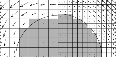
Figure 13: Representation of the inner cylinder (shaded) on a Cartesian mesh for $\delta x=0.067$ (left) and $\delta x=0.033$ (right). Overlayed are the circles of effective radius $R_{1}^{\rm(eff)}$, and arrows representing the velocity field. All lengths are measured in units of $R_{0}$.