Clouds and Chemistry: Ultracool Dwarf Atmospheric Properties from Optical and Infrared Colors

Abstract

The optical and infrared colors of L and T dwarfs are sensitive to cloud sedimentation and chemical equilibrium processes in their atmospheres. The $i^{\prime}-z^{\prime}$ vs. $J-K$ color-color diagram provides a window into diverse atmospheric processes mainly because different chemical processes govern each color, and cloud opacity largely affects $J-K$ but not $i^{\prime}-z^{\prime}$. Using theoretical atmosphere models that include for the first time a self-consistent treatment of cloud formation, we present an interpretation of the $i^{\prime}-z^{\prime}$ vs. $J-K$ color trends of known L and T dwarfs. We find that the $i^{\prime}-z^{\prime}$ color is extremely sensitive to chemical equilibrium assumptions: chemical equilibrium models accounting for cloud sedimentation predict redder $i^{\prime}-z^{\prime}$ colors—by up to 2 magnitudes—than models that neglect sedimentation. We explore the previously known $J-K$ color trends where objects first become redder, then bluer with decreasing effective temperature. Only models that include sedimentation of condensates are able to reproduce these trends. We find that the exact track of a cooling brown dwarf in $J-K$ (and $i^{\prime}-z^{\prime}$) is very sensitive to the details of clouds, in particular to the efficiency of sedimentation of condensates in its atmosphere. We also find that clouds still affect the strength of the $J$, $H$, and $K$ band fluxes of even the coolest T dwarfs. In addition, we predict the locus in the $i^{\prime}-z^{\prime}$ vs. $J-K$ color-color diagram of brown dwarfs cooler than yet discovered.

1 Introduction

The Sloan Digital Sky Survey (SDSS) and the 2-Micron All Sky Survey (2MASS) have both had great success in discovering L and T type ultracool dwarfs. The colors of these objects provide insight into the processes operating in their atmospheres. In the SDSS system, all such objects are uniquely red in $i^{\prime}-z^{\prime}$. L dwarfs are red in the 2MASS $J-K_{s}$ color $(1\leq J-K_{s}\leq 2)$ while the cooler T dwarfs like Gliese 229 B are bluer $(J-K_{s}<0.5)$ (Kirkpatrick et al. 1999; Burgasser et al. 1999; Burgasser et al. 2000). While the mechanisms responsible for the $J-K_{s}$ and the $i^{\prime}-z^{\prime}$ colors of the L and T dwarfs are generally understood, there has yet been no single theory that self-consistently describes the evolution of ultracool dwarfs in this color space.

Because of their intrinsic faintness, moderate to high resolution spectroscopy may not be performed on all of the ultracool dwarfs discovered by these surveys. Thus analyses of ultracool dwarf colors could be essential to provide information on their physical properties. We have explored the utility of a number of $i^{\prime}$, $z^{\prime}$, $J$, $H$, and $K$ color-color diagrams for constraining physical properties and find the $i^{\prime}-z^{\prime}$ vs. $J-K$ diagram particularly interesting. First, these are essentially the colors in which SDSS and 2MASS discover ultracool dwarfs. Second, alkali metals dominate the $i^{\prime}-z^{\prime}$ colors while H₂O and CH₄ absorption bands and cloud physics control the $J-K$ colors. Over the pressure and temperature ranges of interest, the chemical pathways of alkali metals and H₂O/CH₄/CO are not strongly coupled, thus this particular color-color diagram reflects a remarkably diverse set of chemical effects.

In this paper we describe how clouds and the chemistry of carbon, oxygen and alkali elements (mainly potassium) control the 2MASS and SDSS colors used to discover ultracool dwarfs, and we explore the potential of the $i^{\prime}-z^{\prime}$ vs. $J-K$ color-color diagram as a tool to deduce the physical characteristics of dwarfs and the physics of their atmospheres. We also predict the colors of very cool brown dwarfs, those with effective temperatures $T_{\rm eff}\mathrel{\hbox{\hbox to0.0pt{\lower 2.15277pt\hbox{$\sim$}\hss}\raise 1.72218pt\hbox{$<$}}}700\,$K, which are yet to be discovered.

2 Color Trends

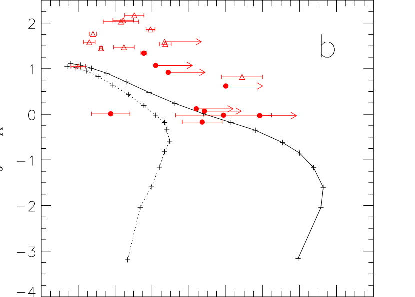
Figure 1: $i^{\prime}-z^{\prime}$ (SDSS) vs. $J-K$ (MKO system) color-color diagrams for L (triangles) and T (circles) dwarfs (Strauss et al. 1999; Fan et al. 2000; Legett et al. 2000; Tsvetanvo et al. 2000; Leggett et al. 2001; Geballe et al. 2001a). Plotted SDSS magnitudes have been converted to the AB system while the MKO magnitudes are in the Vega system. Lower limits are denoted by arrows. The lines show our theoretical models computed in the same systems with the symbols representing $T_{\rm eff}$ steps of 100 K in the $T_{\rm eff}$ range 2000 K – 400 K. Panel (a) shows the results of cloudy models (dashed and dotted lines with $f_{\rm rain}=3$ and 5, respectively) and cloud free models (solid line) for $g=1000\,\rm m\,s^{-2}$. Panel (b) shows cloud free models with $g=1000\,\rm m\,s^{-2}$. The solid line shows models with the sedimentation chemical equilibrium model by Lodders and the dotted line are models using the BS99 chemical equilibrium model with no condensate sedimentation. See §3 and §4 for details. The anomalous data point at $i^{\prime}-z^{\prime}=2.44$, $J-K=0.01$ represents SDSSJ020742.83+000056.2.

Ultracool dwarfs are notoriously different from blackbodies of the same effective temperature. Figure 1 shows the $i^{\prime}-z^{\prime}$ vs. $J-K$ colors for observed SDSS L and T dwarfs (Strauss et al. 1999; Fan et al. 2000; Leggett et al. 2000; Tsvetanov et al. 2000; Geballe et al. 2001a). The ultracool dwarfs are spread out over several magnitudes in both $i^{\prime}-z^{\prime}$ and $J-K$. In addition, they are located in very different parts of this diagram.

Blackbodies become redder in all colors with decreasing $T_{\rm eff}$ as the Planck peak shifts redward; a temperature sequence of blackbody emitters in Figure 1 would follow a diagonal line cutting from blue to red through the extreme upper left corner of the color-color diagram. Ultracool dwarfs, however, are subject to a more complex set of influences and first become redder and then bluer in $J-K$ as they age and cool. The initial reddening arises as progressively larger amounts of condensates are found in the visible atmospheres in the $T_{\rm eff}$ range from $\sim 2000$ to $\sim 1400\,\rm K$. At lower effective temperatures $J-K$ turns blueward because in the cooler brown dwarfs the cloud base (and thus most of the cloud opacity) falls below the photosphere (Marley 2000; Ackerman & Marley 2001; Tsuji 2001; Allard et al. 2001), leaving the visible atmosphere relatively clear of condensates. In the absence of clouds, opacities such as water, methane, and pressure-induced absorption by molecular hydrogen act to rapidly close the $K$ band infrared window as $T_{\rm eff}$ falls, resulting in increasingly blue $J-K$.

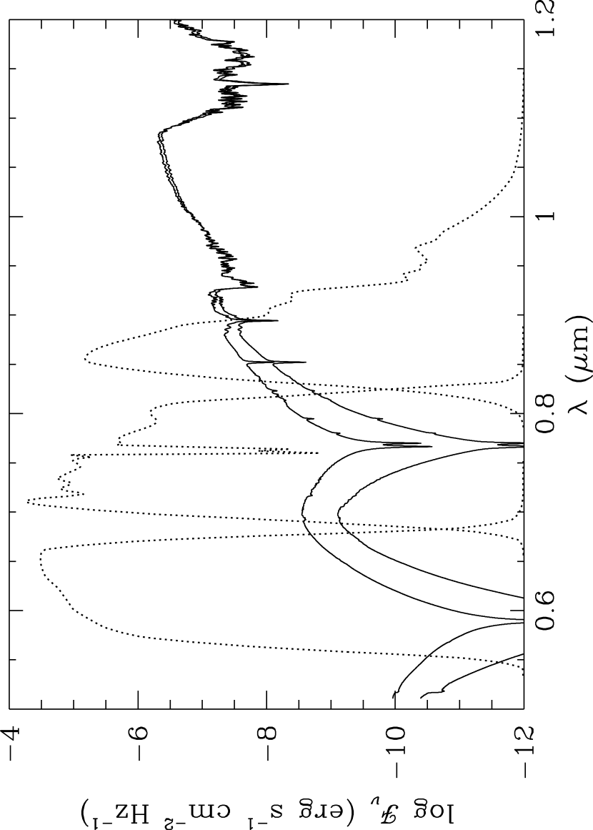
Figure 2: SDSS $r^{\prime}$, $i^{\prime}$, and $z^{\prime}$ transmission curves (dotted lines from left to right, respectively) superimposed on brown dwarf model spectra. The $i^{\prime}$ flux is controlled by the K I doublet line core and the $z^{\prime}$ flux by the K I doublet wing. These cloud free synthetic spectra with $T_{\rm eff}=1000\,$K and $g=1000\,\rm m\,s^{-2}$ are computed with the chemical abundances of BS99 (i.e. no sedimentation assumed; upper curve) and of Lodders (with condensate sedimentation; lower curve). The effect of the chemical equilibrium model on the strength of the K I and Na I doublets is very noticeable. See §3.2 and §4.2 for details.

In the optical, known ultracool dwarfs become redder with decreasing $T_{\rm eff}$. This trend is produced by the growing importance of the $0.59\,\mu$m Na I and $0.77\,\mu$m K I resonance doublets (Tsuji, Ohnaka & Aoki 1999; Burrows, Marley, & Sharp 2000) with decreasing $T_{\rm eff}$; as the dwarf cools, the gradual disappearance of TiO and cloud opacity leaves a progressively more transparent atmosphere at optical wavelengths. The K I resonance doublet is centered on the $i^{\prime}$ band while the $z^{\prime}$ band is only affected by the far red wing, producing very red $i^{\prime}-z^{\prime}$ colors (Fig. 2). We predict below that this trend should reverse in objects with lower $T_{\rm eff}$ than have yet been observed.

Brown dwarfs with $T_{\rm eff}$ and infrared colors intermediate between the coolest and reddest L dwarfs and the much cooler and bluer T dwarfs like Gl 229 B were initially thought to be rare since 2MASS found few of them (Kirkpatrick et al. 2000). T dwarfs with $1100\mathrel{\hbox{\hbox to0.0pt{\lower 2.15277pt\hbox{$\sim$}\hss}\raise 1.72218pt\hbox{$<$}}}T_{\rm eff}\mathrel{\hbox{\hbox to0.0pt{\lower 2.15277pt\hbox{$\sim$}\hss}\raise 1.72218pt\hbox{$<$}}}1300\,$K are difficult to discover in the 2MASS $J-K_{s}$ color because their colors are similar to the far more numerous and hotter M dwarfs. The SDSS optical colors do not suffer from this infrared color degeneracy in this $T_{\rm eff}$ range. The SDSS collaboration found the first brown dwarfs with $J-K$ colors lying between 0.5 and 1 (formerly called L/T transition objects; see Leggett et al. 2000) and has now typed them as early T dwarfs (Geballe et al. 2001a).

3 Model Atmospheres

To model the colors of solar metallicity L and T dwarfs we employ the radiative-convective equilibrium atmosphere model of Marley et al. (1996; further described in Burrows et al. 1997). The model has been updated to self-consistently include both alkali opacities as described in Burrows et al. (2000) and the precipating clouds of Ackerman & Marley (2001). The treatment of the clouds and the chemistry is described further below.

High resolution spectra are computed from these atmosphere models (temperature profile and cloud structure) with a spectral synthesis code (Saumon et al. 2000; Geballe et al. 2001b). In the high-resolution spectra, the non-isotropic scattering by dust particles is mapped onto an equivalent isotropic scattering problem following the prescription given in Chamberlain & Hunten (1987). Theoretical colors in turn are calculated from the high resolution synthetic spectra. For $J$ and $K$ colors we use the Mauna Kea Observatory (MKO) Near Infrared System (Simons & Tokunaga 2001; Tokunaga, Simons & Vacca 2001) and for SDSS the $i^{\prime}$ and $z^{\prime}$ filter functions and the AB magnitude system (Fukugita et al. 1996).

3.1 Cloud Model

For the radiative transfer calculations the clouds are assumed to be horizontally homogeneous and are modeled following the approach developed by Ackerman & Marley (2001). This approach assumes a steady state in which the upward transport of gas and condensate by turbulent mixing is balanced by the downward transport of condensate by sedimentation. In convective regions the turbulent mixing in the model is determined by the convective heat flux, and in radiative regions the mixing is determined by a minimum eddy diffusion coefficient, a prescribed parameter that characterizes such processes as breaking buoyancy waves. The sedimentation (or precipitation) in the model is determined by the condensate mass, the convective velocity, and $f_{\rm rain}$, an adjustable parameter that describes the efficiency of sedimentation relative to the turbulent mixing. Physically, $f_{\rm rain}$ represents the combined effects of unresolved dynamical and microphysical details such as the skewness of atmospheric circulations and the abundance of condensation nuclei. Larger values of $f_{\rm rain}$ correspond to greater precipitation and hence thinner clouds. Note that the base of a cloud is fixed at the lowest level where the partial pressure of a condensible exceeds its saturation vapor pressure. Hence, any precipitation that falls through the base of a cloud is assumed to evaporate, returning its mass to the reservoir of vapor below the cloud. Precipitation through cloud base does not annihilate the cloud; instead the (steady-state) cloud is continually replenished by condensation in updrafts from below, as in long-lived terrestrial clouds.

The value of $f_{\rm rain}$ and the profile of turbulent mixing together determine the profile of condensate mass in the clouds; by assuming that the cloud particle sizes follow a lognormal distribution in a manner consistent with the turbulent mixing and sedimentation, the model also calculates a vertical profile of cloud opacity. Ackerman & Marley (2001) find that their model best fits the observations of condensate scale height, particle size, and optical depth in Jupiter’s ammonia cloud deck with a value of $f_{\rm rain}=3$.

The cloud structure and atmosphere temperature profiles are solved to converge simultaneously and self-consistently by the atmosphere code. As the atmospheric temperature structure as a function of pressure, $T(P)$, is adjusted by the convergence algorithm, a new cloud profile is computed following Ackerman & Marley (2001). In the course of the calculation of a single temperature-pressure profile for a specified $T_{\rm eff}$ and gravity $g$, many hundreds of trial $T(P)$ and associated cloud profiles are computed. An atmospheric structure is not considered acceptable unless both the temperature structure and the cloud model have simultaneously and self-consistently converged .

In this work we include only Fe, $\rm MgSiO_{3}$ (representing both $\rm Mg_{2}SiO_{4}$ and $\rm MgSiO_{3}$), and $\rm H_{2}O$ as condensates. Other species (e.g. $\rm Al_{2}O_{3}$) either condense below the optically thick Fe cloud or are relatively insignificant opacity sources (see Marley 2000). For example, in the $T_{\rm eff}=2000\,\rm K$ model the $\rm Al_{2}O_{3}$ cloud falls in a region of the atmosphere that is already opaque. The additional opacity arising from the cloud does not alter the adiabatic temperature profile. The overlying silicate and iron clouds play a far more important role. For hotter cases where silicates do not condense, $\rm Al_{2}O_{3}$ is more important.

Figure 3 presents several of our temperature-pressure profiles for $T_{\rm eff}=2000$ and 1300 K. For each $T_{\rm eff}$ a cloud free and two cloudy models are shown. Our cloud free models are computed with the same set of assumptions for chemical equilibrium as are our cloudy models (condensed species are segregated by settling and no longer interact with the gas), but with all cloud opacity removed to isolate the effect of the clouds (see §3.2 for comparison with the models of Allard et al. (2001)). Condensation equilibrium curves establish the cloud base level for each profile. Two $T_{\rm eff}=1300\,\rm K$ profiles from Tsuji (2001) are also shown.

For the $T_{\rm eff}=2000\,\rm K$ models silicate and iron grains form above the radiative-convective boundary and their influence on the radiative temperature profile is apparent. The cloudy models are substantially warmer than the equivalent cloud free case. As expected, the (optically and physically) thicker $f_{\rm rain}=3$ cloud produces an even greater thermal perturbation than the case with more efficient sedimentation ($f_{\rm rain}=5$).

In the case of the 1300 K cloudy models, the cloud base is located within the convective region. The temperature profile within this region is set by the adiabatic lapse rate. Since the cloud simply adds to the (already high) opacity and the thermal profile is controlled by the adiabatic lapse rate, perturbations along the atmospheric thermal profile comparable to the hotter case are not seen. The clouds do play a role in raising the top of the convection zone above what it would be in the otherwise identical cloud free case by adding opacity above the cloud-free radiative-convective boundary. Above the cloudy radiative-convective boundary the cloud-top opacity is sufficient to keep the radiative portions of the atmosphere warmer than in the cloud-free case.

The entropy at the radiative-convective boundary controls the adiabat upon which the deeper atmosphere—and consequently the entire interior of the ultracool dwarf—resides (Burrows et al. 1997). The cloudier the upper atmosphere (smaller $f_{\rm rain}$), the hotter the interior. The interior structure at a fixed effective temperature and the amount of energy which must be radiated away to cool the entire dwarf to a lower effective temperature are thus affected by even small differences in cloud opacity. Hence different cloud structure assumptions produce different cooling histories. We plan to explore such effects in a future work.

Different assumptions regarding the cloud models result in very different thermal profiles. For example the cloud free model from Tsuji (2001) shown in Figure 3 is quite similar to our own result for the same $g$ and $T_{\rm eff}$. Also shown is a model from Tsuji (2001) (Tsuji’s case B) in which there is no removal of condensates from the atmosphere above the cloud base. In this case the greenhouse heating of the atmosphere by the abundant dust far exceeds what our cloudy models with sedimentation predict. The upper atmosphere in this $T_{\rm eff}=1300\,\rm K$ case reaches temperatures as high as those found in our cloudiest $T_{\rm eff}=2000\,\rm K$ case. This example dramatically highlights the important role sedimentation plays in moderating what would otherwise be an overpowering role of dust in controlling the temperature-pressure profile of the atmosphere. Chabrier et al. (2000) discuss the dissociation of water occuring in the atmospheres of their hot, dusty no-sedimentation cases (their ‘DUSTY’ models). The large dissociation fractions in those models are simply driven by the lack of any sedimentation and thus represent particularly extreme–and likely unphysical–cases. Although not shown in Figure 3 for the sake of clarity, Tsuji (2000) also presents a ‘unified’ model in which the top of the cloud is simply terminated at an arbitrary temperature. Such a model produces little to no heating in the atmosphere above the cloud top and substantial heating below the cloud top (comparable to our $f_{\rm rain}=5$ case for $T_{\rm eff}=1300\,\rm K$). Ultimately only detailed fitting of observed spectra and colors will distinguish between all such possibilities.

3.2 Chemical Equilibrium Model

The calculation of chemical equilibrium in an atmosphere is dependent upon the assumptions made regarding the fate of condensates. In a gravitational field, atmospheric constituents that condense tend to fall. If the condensate is liquid water meteorologists term it rain. We consider two different chemical equilibrium models. In the first case there is no sedimentation of condensates. For this we use the baseline model from Burrows and Sharp (1999; hereafter BS99). In the second case we treat sedimentation with the cloud condensation model developed by Lewis (1969) for Jovian planets and used by Fegley and Lodders (1996), Lodders (1999), and Lodders and Fegley (2001) for brown dwarfs.

Note that there is a slight inconsistency between the vertical distribution of condensates in the chemical equilibrium model (using the vertical profile described by Lewis (1969)) and the radiative transfer cloud model (using the model of Ackerman & Marley (2001)). However, the vertical condensate profiles with moderate values of $f_{\rm rain}$ are similar to those predicted by the Lewis model. See Ackerman & Marley (2001) for more details.

For the purposes of comparison, we have also computed a sequence of cloud free models. In these models, the presence of condensates is taken into account in the calculation of the chemical equilibrium but the opacity of condensates is ignored in the calculation of radiative transfer. These models differ from the ‘COND’ models of Allard et al. (2001). In the Allard et al. models the chemical equilibrium always assumes the presence of grains even if they are not included in the radiative transfer.

4 The Optical-IR Color-Color Diagram

Figure 1 shows a temperature sequence of ultracool dwarf models in the $i^{\prime}-z^{\prime}$ vs. $J-K$ color-color diagram. Models are plotted for a fixed surface gravity of $1000$ m s^-2, corresponding roughly to a mass of 35 Jupiter masses ($\rm M_{J}$). Note that the surface gravity, $g$, of a given object increases as it contracts and cools, so for a given object the cooling track will follow a slightly different path. Evolution paths for ultracool dwarfs of different masses, however, are almost degenerate in the color-color diagram because the temperature at which optical depth 2/3 is reached as a function of wavelength depends only weakly on the gravity. All surface gravities very nearly overlap in the $i^{\prime}-z^{\prime}$ vs. $J-K$ color-color diagram. So although $T_{\rm eff}$ may be estimated, there is no unique ($T_{\rm eff},g$) solution for given $i^{\prime}-z^{\prime}$ and $J-K$ colors.

The $i^{\prime}-z^{\prime}$ vs. $J-K$ color-color diagram is very sensitive to $T_{\rm eff}$ because of the disparate chemistry governing the two colors. The alkali metal chemistry for the observed ultracool dwarfs shown in Figure 1 mostly consists of neutral K being depleted into molecules and solids. This process (see Lodders 1999 for a complete discussion) is not strongly coupled to the C/H/O chemistry that controls CO, CH₄ and H₂O partitioning. At even lower temperatures, K disappears into chloride and hydroxide gases but the alkali chemistry is still only weakly coupled to the C, H, and O chemistry. As a result dwarfs at different $T_{\rm eff}$ are well separated in this color-color diagram. There is no degeneracy for different $T_{\rm eff}$ as found in most other color-color combinations (e.g. $H-K_{s}$ vs. $J-H$, $J-K_{s}$ vs. $I-J$ (see Kirkpatrick et al. 2000 and Tsuji 2001)).

4.1 Clouds

The behavior of a cloud layer as a function of $T_{\rm eff}$ is of primary astrophysical interest. Qualitatively, the base of the cloud occurs where the $(T,P)$ structure of the atmosphere crosses the condensation curve of the major condensates (silicate and iron at high temperatures, and water at lower temperatures). A cloud deck forms with a vertical profile determined by the cloud model. Because in the region of interest the condensation temperature of relevant substances increases weakly with pressure, the base of the cloud layer occurs at a nearly constant (but slowly increasing) temperature as $T_{\rm eff}$ decreases. On the other hand, the temperature of the photosphere is approximately $T_{\rm eff}$. It follows that as $T_{\rm eff}$ decreases, the cloud layer gradually disappears below the observable level of the atmosphere. This phenomenon has been discussed by several authors (Chabrier et al. 2000; Marley 2000; Allard et al. 2001; Tsuji 2001).

The opacity of the gas in ultracool dwarfs is dominated by molecular bands and varies strongly with wavelength. In contrast Mie scattering by large particles produces a nearly grey cloud opacity. Thus the above discussion is somewhat simplistic since the concept of photosphere is not well defined in these objects. While continuum opacities ensure that the photosphere corresponds approximately to a fixed physical level in normal stars, in brown dwarfs the visible and near-infrared spectrum can probe a range of depths of up to 6 pressure scale heights (Saumon et al. 2000). This range provides an opportunity to observationally probe the vertical structure of brown dwarf atmospheres.

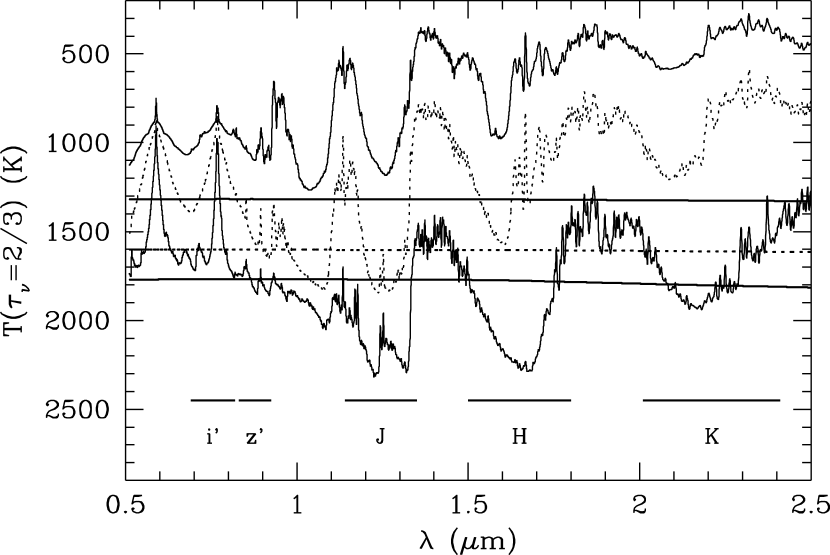
Figure 4: Visibility of the cloud layer in brown dwarfs as a function of $T_{\rm eff}$. The curves show the depth of the photosphere ($\tau_{\scriptscriptstyle\nu}=2/3$), indicated by the temperature in the atmosphere, as a function of wavelength. The abcissa is essentially a brightness temperature. Three models with $g=1000\,$m s^-2 and $f_{\rm rain}=5$ are shown, from top to bottom $T_{\rm eff}=500$, 1000 (dotted), and 1500 K, respectively. Two curves are shown for each model, one showing the photosphere due to gas opacity only, and one due to cloud opacity only. The latter is very flat, due to the nearly grey cloud opacity, and shows the level where the cloud becomes optically thick. At wavelengths longer than shown here, the cloud remains below the photosphere for all models. Bandpasses for several filters are indicated along the bottom of the figure.

The gradual disappearance of the cloud layer below the “photosphere” as $T_{\rm eff}$ decreases is illustrated in Figure 4 where the curves show the level in the atmosphere where the optical depth $\tau_{\scriptscriptstyle\nu}=2/3$. Here, vertical position in the atmosphere is indicated by the local temperature. Three cases are shown with $T_{\rm eff}=500$, 1000, and 1500 K from top to bottom, respectively. A pair of curves is shown for each model; one showing the photosphere (where optical depth $2/3$ is reached) determined by gas opacity only and one for the nearly grey cloud opacity only. For the upper pair of curves ($T_{\rm eff}=500\,$K), the deep silicate and iron cloud “photosphere” lies below (at higher temperature) the gas photosphere at all wavelengths, implying that the cloud layer remains essentially invisible and has little effect on the emergent spectrum. In the lower pair of curves ($T_{\rm eff}=1500\,$K), the cloud becomes opaque well above the gas photosphere in the $J$, $H$, and $K$ bands. The cloud layer is therefore observable in these three bandpasses (but not at other wavelengths) and the spectral energy distribution is strongly affected by the presence of the cloud.

Figure 4 clearly shows that the cloud layer disappears below the observable atmosphere over a range of effective temperatures, depending on the bandpass of observation. For example, the cloud becomes invisible in the $K$ band for $T_{\rm eff}\mathrel{\hbox{\hbox to0.0pt{\lower 2.15277pt\hbox{$\sim$}\hss}\raise 1.72218pt\hbox{$<$}}}1400\,$K but remains detectable in the $J$ band down to $T_{\rm eff}\sim 800\,$K. The Ackerman & Marley cloud model with $f_{\rm rain}=5$ implies that the spectra of all known T dwarfs are affected by clouds.

Observationally, one of the most revealing features in the $i^{\prime}-z^{\prime}$ vs. $J-K$ color-color diagram shown in Figure 1 is the reddening in $J-K$ of the L dwarfs that is not present in the T dwarfs. This difference in $J-K$ trajectory results from the presence of condensates throughout the photosphere of the L dwarfs but not in the late T dwarfs. The blackbody-like condensate emission pushes L dwarfs to the red in $J-K$, despite the tug of water opacity towards the blue. This effect of condensate opacity is best illustrated by comparing the cloud free models and the cloudy models in Figure 1a. The cloud free L dwarf models show a continuous blueward trend in $J-K$ with decreasing $T_{\rm eff}$ — because of increasing H₂O and pressure-induced $\rm H_{2}$ absorption — in contradiction with the redward trend of the L dwarf data. The cloudy models on the other hand, generally match the redward trend in $J-K$ of the L dwarf data.

The progressively redder $J-K$ colors of L dwarfs has been noted before (e.g. Kirkpatrick et al. 1999; Martin et al. 1999; Fan et al. 2000; Leggett et al. 2001; Tsuji 2001) and demonstrated by spectral fitting to be caused by the appearance of more and more silicate condensates in the cooling ultracool dwarf atmospheres (e.g Leggett, Allard, & Hauschildt 1998; Burrows, Marley & Sharp 2000; Chabrier et al. 2000; Marley 2000). However models in which there is no settling of the condensates (Chabrier et al. 2000) produce colors, particularly for the later L dwarfs, that are much too red. For example the dusty model of Chabrier et al. predicts that a 1 Gyr old $50\,\rm M_{J}$ brown dwarf with $T_{\rm eff}=1424\,\rm K$ will have $J-K=3.9$. In fact the reddest L-dwarfs have $J-K\approx 2.2$ (see Fig. 4 of Leggett et al. 2001). Our models with $f_{\rm rain}=3$ peak at $J-K\sim 1.8$ for $T_{\rm eff}=1400\,\rm K$. The muted $J-K$ colors of the reddest L dwarfs provide strong evidence of condensate sedimentation.

A second revealing feature in the $i^{\prime}-z^{\prime}$ vs. $J-K$ color-color diagram is the transition between the L and early T dwarfs that begins as a blueward turnover in $J-K$ in the latest L dwarfs (Leggett et al. 2001). As the condensates sink below the visible atmosphere, their blackbody effect is removed, halting the redward $J-K$ progression. As molecular opacities ($\rm H_{2}$, $\rm H_{2}O$, and later $\rm CH_{4}$) become predominant, their greater absorption at $K$ band initiates the turn in $J-K$ to the blue. This turnover occurs when the cloud layer is no longer visible in the $K$ band (see Fig. 4). An important issue has been the temperature range over which the L to T transition occurs (e.g. Reid et al. 2001). The model $T_{\rm eff}$ at which the turnover begins, as well as the maximum value of $J-K$, depend on the sedimentation parameter $f_{\rm rain}$. Of the models shown in Figure 1, $f_{\rm rain}=3$ comes closest to matching the observed turnover in $J-K$. Smaller values of $f_{\rm rain}$ produce thicker, more massive clouds and somewhat lower values may better fit the peak $J-K$ at the turnover. The cloud tops remain in view in the $J$ and $K$ bands down to cooler $T_{\rm eff}$. This $J-K$ blueward turnover likely will be better characterized by future SDSS discoveries, and the data will be essential for understanding cloud properties in ultracool dwarfs.

At some lower $T_{\rm eff}$ ($\sim 800\,$ K for $f_{\rm rain}=5$) the base of the condensate cloud base is below the visible photosphere. However, the tops of the silicate clouds might still be limiting the depths from which flux emerges in the water and methane windows, thus accounting for the difficulty all cloud free models have had in correctly reproducing the ratio of the flux emerging from within and without of the water bands (Allard et al. 1996; Marley et al. 1996; Tsuji et al. 1996; Saumon et al. 2000; Geballe et al. 2001b).

4.2 Alkali Metal Chemistry

The $i^{\prime}$ and $z^{\prime}$ band fluxes are diagnostic of alkali metal chemistry, mainly because they measure the core and the wing of the K I resonance doublet, respectively. In T dwarfs, the red wing of the doublet is detected up to 200 nm from the line core (Burrows et al. 2000). Figure 2 shows the $i^{\prime}$ and $z^{\prime}$ filters superimposed on two different model spectra. The $i^{\prime}$ filter is centered on the K I doublet core and the $z^{\prime}$ filter probes the far red wing. The ultracool dwarf colors become redder in $i^{\prime}-z^{\prime}$ for decreasing $T_{\rm eff}$ because these filters probe the Wien tail of the Planck function and the K I doublet gets stronger. The gradual disappearance of TiO and cloud opacity as $T_{\rm eff}$ decreases leaves behind a nearly transparent atmosphere at wavelengths below $1\,\mu$m (Figure 4) and reveals the K I doublet in all its pressure-broadened splendor. At low $T_{\rm eff}$ ($\sim 700\,$K) the $i^{\prime}-z^{\prime}$ redward trend halts as K I is depleted into KCl and the doublet weakens.

Given the dependence of the $i^{\prime}-z^{\prime}$ color on the K I resonance doublet, this color provides a stringent test for chemical equilibrium models. The two curves in Figure 1b show colors computed with and without the assumption of condensate sedimentation in the chemical equilibrium calculation. There is a substantial difference — of 2 magnitudes — in $i^{\prime}-z^{\prime}$ at effective temperatures where the K I line is prominent ($\sim 800\,\rm K$). The major difference between the two approaches is that at temperatures below 1400 K, the monatomic K abundance (hence the opacity) is greatly reduced under the assumption of no sedimentation (BS99) compared to the assumption of sedimentation (Lodders 1999). A comparison of spectra computed under both assumptions is shown in Figure 2. The effect on the $i^{\prime}-z^{\prime}$ color is rather dramatic and the models without sedimentation turn blueward well before the model that includes sedimentation, as shown in Figure 1.

Because the SDSS T-dwarfs are only marginally detected in $i^{\prime}$ band, errorbars for those objects shown in Figure 1 are substantial. The trends in T-dwarf data shown in the figure are generally closer to the sedimentation chemistry models, but more and better $i^{\prime}$-band detections are required to fully support this conclusion.

The two different assumptions used to model chemical equilibrium of gas and condensates give such different results that they are worth discussing in more detail. The two models depend on the physical setting (see Lodders 1999; Lodders & Fegley 2001). In the no-sedimentation case condensates remain in local equilibrium with the gas. In cooler regions, the high temperature (primary) condensates react with the upper atmospheric gas to form secondary condensates via gas-solid reactions. Complete chemical equilibrium exists between all phases in this no-sedimentation case. BS99 term this case the “no rainout” approach. Their approach (also employed by e.g. Chabrier et al. 2000; Allard et al. 2001) implies that alkali elements such as Na and K condense into alkali feldspar ((Na,K)AlSi₃O₈) after a long sequence of primary condensate reactions with the gas. The net effect in this no-sedimentation case is that the gaseous atomic K and Na become depleted in the atmosphere once alkali feldspar condenses.

As described in detail by Lodders (1999) and Lodders & Fegley (2001), however, this approach does not apply to ultracool dwarf and giant planet atmospheres because a gravity field is acting on condensates. The primary condensates are sequestered by sedimentation into a cloud and are not available for gas-solid reactions in the atmosphere above the cloud layer as the dwarf cools. These cloud condensation models have been used successfully for over 30 years in the planetary community (Lewis 1969, Barshay & Lewis 1978, Fegley & Lodders 1994) and were recently termed “rainout” by BS99. We prefer to use the term ‘sedimentation’ because ‘rainout’ could be interpretted as implying complete removal. In the sedimentation case, elements such as Al and Ca condense at greater depth and are consequently absent in the overlying atmosphere. Thus alkali feldspar cannot form, and Na and K remain in the gas phase. Only when a brown dwarf is much older and cooler ($T_{\rm eff}\sim 700\,\rm K$) are atmospheric temperatures low enough for monatomic Na and K to convert into chloride and hydroxide gases. At even lower temperatures Na and K condense into $\rm Na_{2}S$ and KCl (see also the discussions in Lodders (1999) and Burrows et al. (2000)).

The $i^{\prime}-z^{\prime}$ color is sensitive to pressure broadening of the K I doublet. The exceptionally strong pressure broadening affecting the $0.59\,\mu$m Na I and the $0.77\,\mu$m K I resonance doublets in T dwarfs stretches the current theories of line broadening beyond their limit of validity. These lines are modeled with a far wing exponential cutoff $\exp-(qh\Delta\nu/kT)$ where $q$ is an undetermined parameter of order unity. A detailed discussion is given in Burrows et al. (2000), as are fits of the optical spectra of Gl 229B and SDSS 1624+00. With abundances determined from the sedimentation chemistry of Lodders (1999), we have obtained good fits of the optical spectra of Gl 229B and Gl 570D with $q=1$ (Geballe et al. 2001b). The $i^{\prime}-z^{\prime}$ color changes by as much as 0.4 mag for models computed with $q=0.5$ and $q=1$. Disentangling the line broadening parameters from other $i^{\prime}-z^{\prime}$ color effects will likely come from fitting high resolution spectra.

4.3 The Coolest Brown Dwarfs

The coolest brown dwarf known with a reliable determination of its effective temperature is Gl 570D with $T_{\rm eff}\sim 800\,$K (Geballe et al. 2001b). Cooler brown dwarfs are expected to enter a new regime in the $i^{\prime}-z^{\prime}$ vs. $J-K$ color space than those discovered so far. Brown dwarfs with $T_{\rm eff}\mathrel{\raise 1.29167pt\hbox{$<$}\mkern-14.0mu\lower 2.58334pt\hbox{$\sim$}}600\,$ K are expected to have water clouds forming in the upper atmosphere. Just as the subsidence of silicate clouds below the photosphere causes a turnover in colors, the appearance of water clouds in the upper reaches of low-$T_{\rm eff}$ atmospheres could have dramatic effects on the colors.

At a relatively cool effective temperature ($\sim 600\,\rm K$), as K I disappears into KCl, the $i^{\prime}-z^{\prime}$ color reaches a maximum and turns blueward as suggested by the coolest objects in Figure 1. The formation of significant ($\tau>0.1$) water clouds below $T_{\rm eff}\sim 500\,$K (depending on $g$) halts and may eventually reverse the blueward march in $J-K$ with decreasing $T_{\rm eff}$ because the water cloud acts like a blackbody, redistributing the flux to the blackbody peak. The models presented here may underestimate the size of the redward turn in $J-K$. Smaller particles than the $\sim 20$ to $30\,\rm\mu m$ predicted by the cloud model would arise for smaller values of the unconstrained stratospheric eddy diffusion coefficient and would produce more cloud opacity for $T_{\rm eff}\leq 500\,\rm K$. Such objects will be very faint at $z^{\prime}$ and will be difficult to detect with SDSS. Nevertheless, the number density of brown dwarfs suggests that a few such objects could be detected by SIRTF (Martín et al. 2001).

5 Discussion

The $i^{\prime}-z^{\prime}$ vs. $J-K$ color-color diagram reveals the importance of precipitating condensation clouds in controlling the colors of the L dwarfs and the transition between L and T dwarfs, and will complement high resolution spectroscopy (Griffith & Yelle 2000; Geballe et al. 2001a) to reveal the nature of condensation chemistry in these atmospheres.

Most previous and current ultracool dwarf models (e.g. Allard et al. 1996; Marley et al. 1996; Tsuji et al. 1996; Burrows et al. 1997; Chabrier et al. 2000; Allard et al. 2001) considered either the case in which condensates remain suspended in the atmosphere or considered them to be absent from the photosphere due to sedimentation. In contrast Marley (2000) and Tsuji (2001) considered cloud decks confined to some fraction of a pressure scale height. The Marley and Tsuji models, although including no cloud physics, were both able to produce a red to blue transition in $J-K$. By including for the first time a self-consistent treatment of cloud physics, we demonstrate that sedimentation processes in clouds result in model $J-K$ colors that are much less red—by up to 2.5 magnitudes—than models with no sedimentation (Chabrier et al. 2000). Sedimentation controls the cloud vertical extent and is responsible for the observed turnover in $J-K$ with decreasing effective temperature. The model further predicts that the spectra and colors of even the coolest known T dwarfs are influenced by clouds.

Furthermore our atmosphere model is the first to compute particle sizes simultaneously and self-consistently with the thermal profile. Both Allard et al. (2001) and Tsuji (2001) assume a fixed, submicron, particle size distribution derived from interstellar medium dust grains. Allard et al. correctly point out that as long as the particle size is smaller than the wavelength of light, Rayleigh scattering dominates the opacities and the exact size distribution of particles has little effect on the opacities. They also argue that particle sizes larger than 100 $\mu$m are implausible because they would break up (terrestrial raindrops and billiard-ball sized hailstones bely this assertion). Our model predicts silicate and iron particle sizes between 10–$100\,\mu$m. Such large particles are Mie, not Rayleigh, scatterers in the near-infrared and possess a completely different spectral opacity (see Figure 3 in Marley (2000)) than the submicron particles assumed by other groups.

The models, however, do not provide a perfect fit to the available data. As noted in section 4.1, the peak model $J-K$ (1.8) is not quite as red as the peak observed value (2.2). L dwarfs with the largest $J-K$ range in $i^{\prime}-z^{\prime}$ from 2.5 to 3.0. At the $J-K$ peak the $f_{\rm rain}=3$ model predicts $i^{\prime}-z^{\prime}=2.1$. This discrepancy may arise from the large uncertainty in the alkali pressure broadening. The value of $f_{\rm rain}$ which comes closest to matching the peak in $J-K$ (observationally an L5 or L6 object, Leggett et al. 2001) does so at a model effective temperature of $1400\,\rm K$. This is slightly cooler than the range expected for such an object (see Burgasser et al. 2001). Of greater concern is that this model then moves too slowly to the blue. The earliest T dwarfs have $J-K\sim 1.3$ (Leggett et al. 2001). The $f_{\rm rain}=3$ model reaches this point at $T_{\rm eff}=1000\,\rm K$ which is certainly too cool. Hence it appears that different values of $f_{\rm rain}$ are required for the early to mid L dwarfs (a Jupiter-like $f_{\rm rain}\sim 3$) and the latest L’s and the T dwarfs ($f_{\rm rain}\sim 5$ or larger) Alternatively Ackerman & Marley (2001) have suggested that holes might preferentially appear in the cloud decks of later type L dwarfs as the clouds begin to form within the convective region of the atmosphere. Bright, relatively blue cloud-free flux emerging from the holes may help hasten the L to T transition in $J-K$. If this is the case a complete description of the disk-averaged emitted flux would by necessity include both relatively cloudy and clear regions.

The optical $i^{\prime}-z^{\prime}$ color is strongly affected by the presence of monatomic potassium and modeling this color relies on the treatment of the alkali condensation chemistry. Chemical equilibrium models not accounting for sedimentation of condensates result in lower KI abundances because potassium is removed from the gas by alkali-feldspar at higher temperatures. Hence the no-sedimentation models yield up to two magnitudes bluer $i^{\prime}-z^{\prime}$ colors than models where sedimentation of condensates is taken into account. This is because the sedimentation of high temperature condensates prevents alkali feldspar from forming and K I abundances are higher until monatomic K is converted into KCl gas and KCl condensation sets in at lower temperatures. Improved brown dwarf $i^{\prime}-z^{\prime}$ colors will reveal which treatment of the equilibrium chemistry in brown dwarf atmospheres is correct. Since the best-fitting cloud model predicts that cloud particles are not lofted much above the cloud base, the sedimentation chemistry is likely most appropriate, in agreement with physically based expectations. A complete test of this hypothesis, however, requires more accurate photometry since brown dwarfs are usually not detected in $i^{\prime}$ band by the SDSS survey. The follow up photometry is in progress.

It is now clear that the interpretation of objects from the warmest L dwarfs to the the coolest T dwarfs requires an understanding of cloud formation in ultracool dwarf atmospheres. Indeed more complex models, motivated perhaps by time resolved photometry and spectroscopy, will be needed to address many fundamental issues. There is no question that what some have termed the field of ‘astrometeorology’ is still in its infancy.

Figure 3: Radiative-convective equilibrium atmosphere models for $g=1000\,\rm m\,s^{-2}$. For two values of $T_{\rm eff}$ solid lines illustrate self-consistent temperature profiles calculated for the case of no cloud opacity (nc) and rainfall efficiency factor $f_{\rm rain}=3$ and 5 (Ackerman & Marley 2001). Lines are labelled for the 2000 K case. For 1300 K the sequence of curves is the same. Triangles denote convective-radiative zone boundaries; the deepest region of the atmosphere is always convective. Dotted lines show 1300 K models by Tsuji (2001) without condensation (left curve) and with condensation but no sedimentation (right curve). Dashed lines show the condensation curves of enstatite and iron.

References

- (1) Ackerman, A. & Marley, M. 2001 ApJ, 556, 872
- (2) Allard, F., Hauschildt, P. H., Baraffe, I., & Chabrier, G. 1996, ApJ, 465, L123
- (3) Allard, F. et al. 2001, MNRAS, in press, arXiv:astro-ph/0104256
- (4) Barshay, S. S. & Lewis, J. S. 1978, Icarus, 33, 593
- (5) Burgasser, A. J. et al. 1999, ApJ, 522, L65
- (6) Burgasser, A. J. et al. 2000, AJ, 120, 1100
- (7) Burrows, A. et al. 1997, ApJ, 491, 856
- (8) Burrows, A., Marley, M. S., & Sharp, C. M. 2000, ApJ, 531, 438
- (9) Burrows, A., & Sharp, C. M. 1999, ApJ, 512, 843 (BS99)
- (10) Chabrier, G., Baraffe, I., Allard, F., & Hauschildt, P. 2000, ApJ, 542, 464
- (11) Chamberlain, J. W. & Hunten, D. M. 1987, Orlando FL Academic Press Inc International Geophysics Series, 36
- (12) Fan, X. et al. 2000, AJ, 119, 928
- (13) Fegley, B. J. & Lodders, K. 1994, Icarus, 110, 117
- (14) Fegley, B. J. & Lodders, K. 1996, ApJ, 472, L37
- (15) Fukugita, M., Ichikawa, T., Gunn, J. E., Doi, M., Shimasaku, K., & Schneider, D. P. 1996, AJ, 111, 1748
- (16) Geballe, T. et al. ApJ, in press, arXiv:astro-ph/0108443
- (17) Geballe, T. R., Saumon, D., Leggett, S. K., Knapp, G. R., Marley, M. S., & Lodders, K. 2001b, ApJ, 556, 373
- (18) Griffith, C. & Yelle, R. 2000, ApJ, 532, L59
- (19) Kirkpatrick, J. D. et al. 1999, ApJ, 519, 802
- (20) Kirkpatrick, J. D., Reid, I. N, Liebert, J., Gizis, J. E., Burgasser, A. J., Monet, D. G., Dahn, C. C., Nelson, B, & Williams, R. J. 2000, ApJ 120, 447
- (21) Leggett, S. K., Allard, F., & Hauschildt, P. H. 1998, ApJ, 509, 836
- (22) Legget, S. K. et al. 2000, ApJ, 536, L35
- (23) Lewis, J. S. 1969, Icarus, 10, 365
- (24) Lodders, K. 1999, ApJ, 519, 793
- (25) Lodders, K. & Fegley, B. 2001, Icarus, in press
- (26) Marley, M. 2000, From Giant Planets to Cool Stars, ASP Conference Series, Vol. 212. Edited by C.A. Griffith and M.S. Marley. (San Francisco: ASP), p.152
- (27) Marley, M. S., Saumon, D., Guillot, T., Freedman, R. S., Hubbard, W. B., Burrows, A., & Lunine, J. I. 1996, Science, 272, 1919
- (28) Martín, E. L., Delfosse, X., Basri, G., Goldman, B., Forveille, T., & Zapatero Osorio, M. R. 1999, AJ, 118, 2466
- (29) Martín, E. L., Brandner, W., Jewitt, D. C., Simon, T., Wainscoat, R., Connelley, M., Marley, M., & Gelino, C. 2001, PASP, 113, 529
- (30) Reid, N. et al. ApJ, in press
- (31) Saumon, D., Geballe, T. R., Leggett, S. K., Marley, M. S., Freedman, R. S., Lodders, K., Fegley, B., & Sengupta, S. K. 2000, ApJ, 541, 374
- (32) Simons, D. & Tokunaga, A. 2001, PASP, in press, arXiv:astro-ph/0110594
- (33) Strauss, M. et al. 1999, ApJ, 522, L61
- (34) Tokunaga, A., Simons, D., & Vacca W. 2001, PASP, in press arXiv:astro-ph/0110593
- (35) Tsuji, T., Ohnaka, K., Aoki, W., & Nakajima, T. 1996, A&A, 308, L29
- (36) Tsuji, T., Ohnaka, K., & Aoki, W. 1999, ApJ, 520, L119
- (37) Tsuji, T. 2001, in press, arXiv:astro-ph/0103395
- (38) Tsvetanov, Z. I. et al. 2000, L61