Spectral classification of stars using synthetic model atmospheres

Abstract

We devised a straightforward procedure to derive the atmosphere fundamental parameters of stars across the different MK spectral types by comparing mid-resolution spectroscopic observations with theoretical grids of synthetic spectra.

The results of a preliminary experiment, by matching the Gunn and Stryker (1983) and Jacoby et al. (1984) spectrophotometric atlases with the Kurucz (1995) models, are briefly discussed. For stars in the A-K spectral range, effective temperature is obtained within a 1-2% relative uncertainty (at 2-$\sigma$ confidence level). This value raises to 4-5% for the hottest stars in the samples (O-B spectral types). A poorer fit is obtained throughout for stars cooler than 4000 K mainly due to the limiting input physics in the Kurucz models.

¹Università degli Studi, via Celoria 16, 20133 Milano, Italy ²Osservatorio Astronomico di Brera, via Bianchi 46, 23807 Merate, Italy ³Telescopio Nazionale Galileo, A.P. 565, 38700 S/Cruz de La Palma (Tf), Spain

1 Introduction

A confident estimate of the atmosphere fundamental parameters of stars is of crucial importance in a number of physical problems dealing with the study of the stellar populations in the Milky Way and the other external galaxies. As a complement of the natural approach, that relies on high-resolution spectroscopy of single objects, one could also try to take advantage of the piece of information provided by mid-resolution observations. The latter can in general probe spectral energy distribution (SED) of stars over a wider wavelength range, and allow us to collect data in a much shorter observing time. Physical information on target stars would derive in this case from a “suitable” comparison with reference spectra (both theoretical and/or empirical ones) searching for a best fit over the whole observed SED.

In this work we propose a simple procedure to derive stellar fundamental parameters (i.e. $T_{\mathrm{eff}}$, $\log{g}$, [M/H]) by matching mid-resolution ($\sim 5$ Å FWHM) observations with a grid of theoretical model atmospheres. The fitting algorithm will be presented in Sec. 2 while some preliminary results of our method will be discussed in Sec. 3.

The Gunn & Stryker ([1983], hereafter GS83) and the Jacoby et al. ([1984], JHC84) spectrophotometric atlases provided the wide sample of target stars (336 in total) for our experiment, with different spectral type (from O to M) and MK luminosity class (from I to V). This allowed us to test our procedure across the whole HR diagram.

The 175 GS83 SEDs are defined in 503 points between 3160 and 10620 Å, with a step of 10 or 20 Å. This coarse sampling basically sets also the intrinsic spectral resolution of the data. Absolute fluxes are given in the AB magnitude scale (Oke & Gunn 1983). The 161 JHC84 SEDs are sampled in 2799 points between 3510 and 7427 Å, by steps of 1.4 Å. They have been obtained at a resolution of 4.5 Å FWHM. Both samples of stars were originally corrected for interstellar reddening.

As a reference framework for our procedure, we relied on the ATLAS 9 synthetic models by Kurucz ([1995]). Other theoretical databases could in principle be used, of course, like for instance the recent and more elaborated NextGen 5 models by Hauschildt et al. ([1999a], [1999b]; see Bertone et al. 2001 for a critical discussion in this regard).

The adopted ATLAS 9 grid consists of 409 models in total, assuming a solar metallicity, a microturbulent velocity of 2 km/s and a mixing-length-to-scale-height ratio L/H_p=1.25. Effective temperature spans the range $50\,000\geq T_{\mathrm{eff}}\geq 3500$ K with a step in the model grid of 250 K for stars cooler than 10 000 K, increasing up to 2500 K for warmer stars. Surface gravity explores the range $0.0\leq\log{g}\leq 5.0$ dex at steps of 0.5 dex. All these model atmospheres and spectra are available on the Internet at the Kurucz www site (http://cfaku5.harvard.edu/).

2 The fitting algorithm

Our method basically consists in a measure of the likelihood function, $s$, that quantifies the similarity between target spectrum and each template SED of the reference grid. As far as the quantity $s$ is known across the grid, that is as a function of the physical parameters of the model atmospheres, a formally “best” solution is identified by the minimum of $s$ in the ($T_{\mathrm{eff}}$, $\log{g}$, [M/H]) parameter space. The underlying hypothesis of this choice is of course that similar spectra are produced by similar physical parameters in a univocal way.

Operationally, the fiducial atmosphere parameters for the i-th star in our target sample are obtained in three steps:

i) we first compute a residual function, $X$ vs. $\lambda$ in the flux logarithm domain such as

$$X_{(i,j)}(\lambda)=[\ln f_{i}(\lambda)-\ln f_{j}(\lambda)]\ W(\lambda)$$ (1)

where $f_{i}$ is the SED of the target star, $f_{j}$ is that of the j-th reference model atmosphere and $W$ is a weighting factor that only depends on $\lambda$. In case a wavelength resampling is necessary to consistently match target and template spectra, this will always be done by rebinning the template spectrum at the wavelength values of the target. We also assume that the template spectrum has been preliminarily degraded to the same resolution of the target data.

ii) We therefore compute the standard deviation of the statistical variable $X$ within the wavelength range of the target observations:

$$\sigma(X)_{(i,j)}=\sqrt{{\it Var(X)}}$$ (2)

As in eq. (1) we worked in the natural logarithm domain, $\sigma(X)_{(i,j)}$ can be read, to a first approximation, as a mean percent deviation of the j-th template spectrum with respect to the i-th target spectrum.

iii) For each template we therefore compute the corresponding likelihood function, $s$, defined as

$$s_{(i,j)}=\sigma(X)_{(i,j)}.$$ (3)

The minimum of the quantity $s_{(i,j)}$ across the grid of reference spectra will eventually identify the “best” fiducial atmosphere parameters for the i-th target star. As a further refinement, to increase the accuracy of our fitting algorithm, we actually search for a minimum of the $s_{(i,j)}$ function after a spline smoothing.

An example of our procedure for star no. 35 (an F6V dwarf) and no. 100 (a K3III giant) in the JHC84 atlas is shown in Fig. 1. In order to estimate the statistical uncertainty in the fiducial set of atmosphere parameters, for each target star we performed an $F$ test on the likelihood function $s$ (the freedom degrees in this case are the number of SED points accounted in the fit). The resulting 2-$\sigma$ confidence interval for a one-tail $F$ test then translates into a confidence range for $T_{\mathrm{eff}}$ and $\log{g}$, as displayed in Fig. 1.

Fig. 1.—: Spline interpolation of the loci of the points $s$ vs. $T_{\mathrm{eff}}$ for two stars in the JHC84 atlas. The solid line is the curve at the best fiducial gravity ($\log g=4.0$ for JHC84 no.35 and $\log g=2.0$ for JHC84 no.100); the dashed lines are the curves at the other surface gravity values; diamonds are the interpolated $s$ values at the best gravity (the points at other gravities have the same abscissas); the square indicates the minimum of the curve. The horizontal dotted line shows the upper limit $s_{\mathrm{max}}$ of the 2-$\sigma$ confidence interval of the standard deviation, given by the $F$ test. This limit defines the $T_{\mathrm{eff}}$ error range, indicated by the vertical dotted lines. The error on $\log{g}$ is provided by the gravity value of the curves that pass under $s_{\mathrm{max}}$.

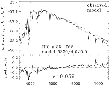
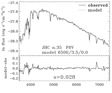
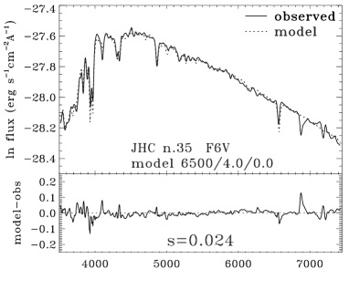
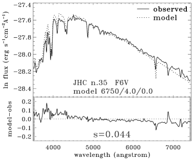
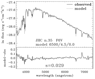
Fig. 2.—: The SED of the star JHC84 no.35 (SAO 57199, F6 V) is compared with several ATLAS9 SEDs. In the left column, the models have same gravity and $\Delta$$T_{\mathrm{eff}}$=250 K. In the right column, the models have same $T_{\mathrm{eff}}$ and $\Delta$$\log{g}$=0.5 dex. The lower panels show the value of $X_{(i,j)}(\lambda)$ (see eq.(1)).

Full details of the matching procedure for the same star no. 35 of Fig. 1 are also reported in Fig. 2, by comparing with Kurucz templates with different temperature (left panels) and surface gravity (right panels). The central panel in the figure is the best fit for $T_{\mathrm{eff}}$= 6500 K and $\log{g}$= 4.0 dex, assuming a solar metallicity.

As far as the continuum emission is concerned, note that the trend in the residual flux is much more sensitive to a change in temperature while any change in gravity would especially reflect in the ultraviolet emission shortward of the Balmer break.

Some artificial features appear in the GS83 spectra about 7600 Å and 9400 Å. They are due to telluric absorption and have therefore been excluded in our analysis by setting W=0 in eq. (1) for the relevant wavelength. In addition, also the region shortward of 3500 Å has been rejected for the same sample due to a poorer flux calibration of the original data in the ultraviolet wavelength range.

3 Results and discussion

As our method entirely relies on the Kurucz synthetic models, its performance is mainly determined by their properties, virtues and faults. The ATLAS 9 models are LTE, plane-parallel and they use the mixing-length theory with overshooting for the treatment of convection. A huge amount of atomic and molecular lines are considered, but triatomic molecules are not implemented in the opacity calculations, and Kurucz (1993) himself suggests not to use these models for M stars.

For 293 out of 336 stars in the GS83 and JHC84 atlases our procedure converged to an acceptable set of fiducial atmosphere parameters (namely $T_{\mathrm{eff}}$ and $\log{g}$, assuming a solar metallicity). About 85% of these stars have $s_{\mathrm{min}}<0.07$, with a mean of 0.05 for the total sample. All stars with poorer fit (i.e. $s_{\mathrm{min}}>0.11$) are cooler than 4000 K. For 43 stars no solution was found as $s_{\mathrm{min}}$ presumably located beyond the physical boundaries of the model grid. They are mostly O and M stars, that is at the extreme edges of the temperature scale. Molecular contribution seems the most likely responsible for the trouble with M stars, while for O stars this seems rather to deal with the non-LTE regime affecting stellar atmospheres at hotter temperature.

Figure 3 gives a summary of our results by reporting the relative uncertainty in the derived $T_{\mathrm{eff}}$ for the 293 stars with fitting solution. The GS83 stars provided slightly better results compared with the JHC84 sample because of a wider wavelength baseline of the spectra that allowed a more accurate determination of $T_{\mathrm{eff}}$. The tipical relative uncertainty (at 2-$\sigma$ confidence level) in the temperature estimate for A-K stars turns about $\pm$ 1-2%, raising to 4-5% for B stars. The typical error box for the surface-gravity estimates is $\pm 0.5$ dex.

Fig. 3.—: Relative error on the $T_{\mathrm{eff}}$ of the stars of the two atlases. The typical 2-$\sigma$ absolute error is $\pm$50–100 K for K-F stars, $\pm$100–200 K for A stars and $\pm$400–1000 K for B stars.

As a final remark, it is worth stressing that our procedure could in principle work also for high-resolution spectra. Different problems would come out in this case, however, deserving to be preliminarily assessed in order to assure a confident fit to the data.

From the operational point of view we know, in fact, that the calibration of echelle spectra at a high-order dispersion is a more critical task to perform over a wide wavelength baseline compared to corresponding low-resolution observations. Computation of theoretical spectra at high-resolution is on the other hand very time consuming, and template grids are usually not available for public release. Furthermore, they take a huge amount of disk space and often cannot be so easily managed with the current computing facilities.

A suitable compromise in this sense could rely on a selective analysis of narrow-band spectrophotometric indices, like in the the Lick system (Worthey et al. [1994]) or according to Rose’s ([1994]) studies, taking full advantage in this case of the high-resolution piece of information but restraining the analysis only to much reduced (and strategically placed) windows to probe the stellar SED.

References

- 2001 Bertone E., Buzzoni A., Chavez M., & Rodriguez L., 2001, in Proc. of “The link between stars and cosmology”, eds. M. Chavez, A. Bressan, A. Buzzoni and D. Mayya, Kluwer, Dordrecht, in press
- 1983 Gunn J.E. & Stryker L.L., 1983, ApJS, 52, 121
- 1999a Hauschildt P.H., Allard F. & Baron E., 1999, ApJ, 512, 377
- 1999b Hauschildt P.H., Allard F., Ferguson J., Baron E. & Alexander D.R., 1999, ApJ, 525, 871
- 1984 Jacoby G.H., Hunter D.A. & Christian C.A., 1984, ApJS, 56, 257
- 1993 Kurucz R.L., 1993, in Proc. IAU Symposium 149, eds. B. Barbuy and A. Renzini, Kluwer, Dordrecht, p.225
- 1995 Kurucz R.L., 1995, CD-ROM n.13, revised
- 1983 Oke J.B. & Gunn J.E., 1983, ApJ, 266, 713
- 1994 Rose J.A., 1994, AJ, 107, 206
- 1994 Worthey G., Faber S.M., González J.J. & Burnstein D., 1994, ApJS, 94, 687