A self-regulated model of galactic spiral structure formation

Abstract

The presence of spiral structure in isolated galaxies is a problem that has only been partially explained by theoretical models. Because the rate and pattern of star formation in the disk must depend only on mechanisms internal to the disk, we may think of the spiral galaxy as a self-regulated system far from equilibrium. This paper uses this idea to look at a reaction-diffusion model for the formation of spiral structures in certain types of galaxies. In numerical runs of the model, spiral structure forms and persists over several revolutions of the disk, but eventually dies out.

I Introduction

The problem of how spiral structures form in galaxies is one that has often been studied (for a general overview of the subject, see [1]), and can be divided into two aspects. The first is that of temporary structures most likely caused by gravitational perturbations from passing galaxies or an asymmetric halo, or disk material having an initial velocity relative to the local standard of rest from formation processes. Here the phenomenon seems to be related to density waves [2], quasi-stable modes in the gravitational potential of the disk which offer a good description of grand design spirals, where the arms are well-defined and has a high degree of symmetry. However, this paper is devoted to the second part of the problem, namely, that of spiral structures in “isolated” galaxies, i.e. where we ignore influences from outside the disk and consider only internal (and recurring) mechanisms. These galaxies can be represented by flocculent spirals, so called because of the fleecy appearance of their many short and asymmetric spiral arms. Because these spirals are seen in blue light, but not red [4] – suggesting the arms are composed of younger, bluer stars, while the older, redder stars are more evenly distributed across the disk – they must be an artifact of star formation itself, and are not primarily density waves. Our attitude here is to consider structure formed by the processes of star formation and neglect gravitational influences. This should apply equally to all spirals, although for grand design spirals, we would expect it to act with density waves arising from other sources.

Most of the theoretical work done in star formation processes deals with the solar neighborhood (those stars in the vicinity of our Sun) as opposed to structures on a galactic scale [5]. Other models used to study these aspects of star formation and spiral structure, such as those built on propagating star formation [6], either greatly simplify the physics involved or need finely tuned parameters to match observations. In this paper, we give a model of spiral structure in isolated galaxies based on the idea of star formation as part of a network of self-regulated and autocatalyzed reactions [7, 8]. Recently, there has been a great deal of both theoretical and experimental work studying how non-equilibrium systems in chemistry and biology produce patterns in both time and space. This has included looking at both the organic – such as bacterial colonies [9], the differentiation of cell types [10], and the formation of embryonic structure in multicellular organisms [10] – as well as the inorganic – the BZ chemical reaction [11], diffusion limited aggregation [12], and self-organized critical systems [13]. There have been many successes in reproducing patterns in the laboratory, and these models typically share both partial differential equations and discrete elements such as cellular automata. However, most of this work in non-equilibrium systems has been after the main work on the formation of structures in astronomy.

Thus one might seek to apply this work to patterns seen in spiral structures. Because we are studying the process in isolated galaxies, we know that the formation must be caused by events within the disk, rather than by the actions of outside players. The isolated galactic spiral is far from equilibrium – there is differentiation of material into stars and clouds of gases whose distribution varies over space and time. In addition, star formation happens at a constant rate, as averaged across the disk. This is a clue that the process is regulated by a feedback loop to maintain this constancy (for evidence of this mechanism, see [15]). These characteristics are shared by other types of non-equilibrium systems. Below, we list the predominant features that these kinds of networks of reactions have in common, along with examples of the same behavior in galactic disks.

• Steady state system  There is a slow (relative to the dynamical time scales) and steady flow of energy, and perhaps matter running through the disk. In spiral galaxies, star formation proceeds at a constant rate, averaged over the disk, for time scales on the order of 10¹⁰ years. The fact that this is greater than the time scales of the actual star formation process (10⁷ years) implies that the slow and steady rate is regulated by feedback mechanisms.

• Non-equilibrium system  The steady state is far from thermodynamic equilibrium, and there is a coexistence of several species or phases of matter, which exchange matter and energy among themselves through closed cycles. The galactic disk is not a uniformly dense clump of material at thermal equilibrium, but instead is divided into gases at different temperatures and stars of various mass. These species exchange matter: for example, massive stars supernova to form warm gas, which can cool and then condense into new stars.

• Feedback mechanisms  The rates at which material flows around these cycles are governed by feedback loops that have arisen during the organization of the system into the steady state. An example of this is suggested by Parravano and collaborators [16] which explains how the average pressure in the interstellar medium (ISM) is maintained. They argue that there are two phases, the warm gas of the ambient phase, and the cooler gas of the condensed phase, with a phase boundary in the pressure-temperature plane. Ultraviolet radiation from the supernovae of massive stars heats the gas, which prevents the condensation of newer stars, so the supernova rate goes down, allowing new massive stars to form (and so the supernova rate will increase again). This feedback mechanism keeps the gas on the phase boundary.

• Autocatalytic reaction networks  Any substances that serve as catalysts or repressors of reactions in the network are themselves produced by reactions inside the network. Suppose we look at the condensation of giant molecular clouds (GMCs). This is catalyzed by dust grains produced by cool giant stars, shielding the clouds and providing sites for molecular binding, and carbon and oxygen, which may cool the clouds by radiation from the rotational modes of CO molecules. The condensation is inhibited by ultraviolet radiation from massive stars, as described by the Parravano process mentioned above.

• Separation in space  There may be spatial segregation of the different phases or materials in the cycles. This occurs when the inhibitory and catalytic influences propagate over different distance scales. At the smallest scale, this means the production of certain substances may be subject to refractory periods – once production has occurred in a local region, it will not be repeated there for some period of time. For the influences in the process of GMC condensation, dust grains, carbon and oxygen propagate only over distances of about 100 parsecs (how far supernovae and massive stars can spread their products) while UV radiation can travel over much of the galactic disk.

As can be seen, there is evidence that we can think of spiral structure in isolated galaxies to be a product of a self-organized, autocatalyzed network of reactions in the star formation process. Given a system with the characteristics listed above, there are models which can describe the spatial structure, the most typical of which is the reaction-diffusion model [10, 17], and we develop a model along these lines for spiral structure in isolated galaxies.

II Theoretical aspects

A One-zone model

We briefly outline the processes necessary to start star formation. The cold clouds of the GMCs condense out of the interstellar medium (ISM), forming distributions of gas and dust that are apparently scale-invariant. As mentioned above, the condensation is helped along by the actions of dust, carbon and oxygen, while it can be impeded by UV radiation from massive stars. The Parravano process may place some limitations on the amount of condensation. Typical time scales for the inhibition are about $10^{7}$ years, the average life span of massive stars, after which the supernova (SN) rate and the UV radiation flux will die off. Once the GMCs start to condense, then their cores may collapse to form stars. This collapsing is brought on by shockwaves from supernovae or HII regions (we neglect any impact that density waves may have in these collapses), and so have the same length scale as the propagation of dust by supernovae, or about 100 parsecs. Once the stars are formed, they can inhibit the infall of gas by the stellar wind or UV radiation produced by the star [18]. These effects occur on short length scales, about the size of one cloud complex, and reduce the star forming efficiency of the clouds down to a few percent.

We must take the processes occurring in the galactic disk and abstract them to produce a viable mathematical model. One way we can simplify the system is to take the continuous spectrum of star types and break it up to those massive stars that can supernova (and thus provide matter and radiation back into the system) and those lighter stars that cannot. We will be neglecting the fact that these lighter stars can return matter to the ISM, so in our model, they will simply act as a matter sink. There is also matter exchange between the cold gas of the GMCs and the warmer ambient gas, due to heating and cooling. We can summarize the flows of material in Fig. 1, and the various material and energy components are given in Table I. Now we give a brief description of the physical processes we include in the model.

• Cloud destruction $cs\to g,cs\to s$: Because of the presence of massive stars and their stellar winds and SNe produced shocks, there will be a mechanism of cloud distruption. Some of this pressure will trigger star formation $(cs\to s)$, but the eventual result will be the disruption of the cloud into warm gas $(cs\to g)$. Typically, the efficiency of star formation is around a few percent.

• Cloud-cloud collisions $c^{2}\to g,c^{2}\to s$: Another source of pressure is the collision of clouds, which will have the same types of effects as the star-induced cloud destruction mentioned above. Again, the rate of star formation is a few percent.

• Mass infall to the disk $\delta$: Galaxies are believed to be formed from the condensation of matter from a spherical halo into a disk, and so there is certainly the possibility that there is a continuing flow of matter. It is believed that the rate is enough to replenish the material in the disk in a time span of billions of years (see Section 4.3 of Larson [19]).

• Direct cloud destruction by stars $cs\to g$: This represents the effects of stars, such as stellar winds, which come directly from the massive stars, as opposed to radiation and shockwaves, which might travel some distance. The main physical action behind this term is the ionization and champagne flows of stars formed inside the cloud [20].

• UV radiation, shockwave production $s\to r,s\to h$: The sources of UV radiation and shockwaves are from SN events from massive stars. These effects are more long range, although shocks will travel only about 100 pc, while radiation can traverse the entire galaxy.

• Damping terms $(c+g)r\to r,(c+g)h\to h$: Because the energy carried by UV radiation and shockwaves will be dissipated by the interaction with matter – both warm and cold – we include a damping term.

• Cooling term $g^{2}/r\to c$: UV radiation will act as a thermostat, since warm gas is less likely to cool in an environment with a high radiation density. In the results presented here, we consider cooling which is inversely proportional to the radiation density.

• Cloud destruction by UV radiation and shockwaves $cr\to g,ch\to s$: These effects are more long-range than the direct cloud destruction used previously. Note that ultraviolet radiation will ionize the clouds into warm gas, as does the destruction induced by massive stars, but the pressure due to shockwaves will initiate new star formation.

Now, we take this model of the material flows in the galactic disk, and write them in a system of equations using the law of mass action – that is, the change in time of the output quantity is given by the product of the densities of the inputs, with a constant parameter giving the rate of the reaction. Thus, given the processes outlined above, we have

$$\frac{dc}{dt} = \frac{\alpha_{1}g^{2}}{r}-\alpha_{2}cr-\beta_{1}ch-\gamma cs-\epsilon_{1}c^{2}$$ (2)

$$\frac{dg}{dt} = -\frac{\alpha_{1}g^{2}}{r}+\alpha_{2}cr+s+\gamma cs+\epsilon_{2}c^{2}+\delta$$ (3)

$$\frac{ds}{dt} = \beta_{2}ch+\epsilon_{3}c^{2}-s$$ (4)

$$\frac{dr}{dt} = \eta_{1}s-\phi_{1}(c+g)r$$ (5)

$$\frac{dh}{dt} = \eta_{2}s-\phi_{2}(c+g)h$$ (6)

$$\frac{dd}{dt} = \beta_{3}ch+\epsilon_{4}c^{2}$$ (7)

where the parameters of the equations $\alpha_{1},\alpha_{2},\cdots$ and their ranges are given in Table II. To choose the parameters, we use the lifetime of a typical massive star, $10^{7}$ years, as the dimension of time, and the units of mass and energy to be those appropriate for each components – for example, we choose the mass unit for warm gas $g$ to be one hydrogen atom per cubic centimeter. Then each parameter is the rate of the reaction at the mass and energy densities we select, e.g. since the mass flow into the galaxy is estimated to completely replace the current material in $10^{10}$ years, we choose the mass inflow constant $\delta\sim 0.001$. For a fuller discussion of the choices made, see [7]. Finally, note that conversation of matter implies $\beta_{1}=\beta_{2}+\beta_{3}$ and $\epsilon_{1}=\epsilon_{2}+\epsilon_{3}+\epsilon_{4}$.

As mentioned above, only massive stars are adding material to the ISM, through the mechanism of supernovae – we are ignoring the fact that light stars add material via evaporation. There are a few other simplifications which have been used to arrive at these equations, such as neglecting the impact of catalyzers to GMC condensation such as dust and carbon to avoid parameters that depend on metal concentrations. Also, we noted previously that our cooling term is inversely proportional to the radiation density. This gives the simple result that cooling is faster when there is less radiation, but this is certainly not the only possibility (although it is the one we have examined more closely). Another choice would be to include something like a step function – once the UV radiation is lower than a certain amount, the rate of cooling increases greatly, but above the cutoff, it is negligible. This idea of a critical density is essentially the process advocated by Parravano and collaborators. However, it can be shown [7] that there is little variation in the average values of the components as the functional dependence of the cooling is altered. In addition, the use of a step function in the cooling function can lead to oscillatory behavior in the components that is almost discontinuous and is therefore undesirable.

B Reaction-diffusion model

The system of equations $(\ref{eqns-one-zone})$ can be useful in understanding such things as the chemical evolution in a galaxy, but there already exists a substantial literature on one-zone models in galactic evolution. Our goal here is to work with a model, similar to those in chemical and biological non-equilibrium systems, where spatial and temporal patterns are generated. In these systems, there are different length scales: L_long is the scale of the whole disk, the distance that UV radiation can travel; L_int is the scale of distances between cloud complexes, and the distance core collapse is induced by supernovae; and L_short is the scale of a single cloud, the distance new stars evaporate the GMC from which they condensed. Note that the reactions characterized by L_int are catalytic, whereas those of L_long and L_short are inhibitive.

To incorporate the effects of these length scales and the inhomogeneities they produce, we introduce diffusion terms into the system of equations. Although diffusion is clearly appropriate for such things as the movement of material such as stars and clouds through the disk, it might seem more realistic to use a wave equation to represent the effects of shockwaves and radiation. However, as is well-known, there are wavelike solutions to reaction-diffusion equations, such as the prototype Fisher equation [21]. Also, we can see from the success the cellular automata of Gerola, Seiden and Schulman [6] and the model of Elmegreen and Thomasson [22] that this is a valid approach.

Because the scale height of the Milky Way is much smaller than that of the radius of the disk, we consider the model on a two-dimensional annulus, leaving out the galactic bulge since it has little influence on the star formation in the disk. Therefore the component functions we considered in Sec. II A are now functions of the radius $\rho$ and the angle $\theta$, in addition to time $t$:

$\displaystyle c=c(\rho,\theta;t)\qquad g=g(\rho,\theta;t)\qquad s=s(\rho,\theta;t)\qquad r=r(\rho,\theta;t)\qquad h=h(\rho,\theta;t)$

Note that the radius and angle, along with the angular velocity $\omega(\rho)$ in the disk, will be the only Greek letters that are not parameters of the model. Being in a rotating system, with angular velocity $\omega(\rho)$, we must use the convective derivative, so that the evolution of the components is given by

$$\frac{\partial c}{\partial t}+\omega(\rho)\frac{\partial c}{\partial\theta} = \frac{\alpha_{1}g^{2}}{r}-\alpha_{2}cr-\beta_{1}ch-\gamma cs-\epsilon_{1}c^{2}$$ (9)

$$\frac{\partial g}{\partial t}+\omega(\rho)\frac{\partial g}{\partial\theta} = -\frac{\alpha_{1}g^{2}}{r}+\alpha_{2}cr+s+\gamma cs+\epsilon_{2}c^{2}+\delta$$ (10)

$$\frac{\partial s}{\partial t}+\omega(\rho)\frac{\partial s}{\partial\theta} = \beta_{2}ch+\epsilon_{3}c^{2}-s+D_{s}\nabla^{2}s$$ (11)

$$\frac{\partial r}{\partial t}+\omega(\rho)\frac{\partial r}{\partial\theta} = \eta_{1}s-\phi_{1}(c,g,r)+D_{r}\nabla^{2}r$$ (12)

$$\frac{\partial h}{\partial t}+\omega(\rho)\frac{\partial h}{\partial\theta} = \eta_{2}s-\phi_{2}(c,g,h)+D_{s}\nabla^{2}h$$ (13)

where the parameters have the same meaning as before, in the one-zone model.

III Numerical results and conclusions

Now that we have our model, we want to know if there are any structures of the right size that will arise. To do this, we consider a linearization of the model, and see if there are any instabilities. We assume that the galaxy is two-dimensional to simplify the analysis, and expand equations $(\ref{eqns-react-diff})$ to linear order around the steady state (i.e. $c={C_{0}}+C+\cdots$, and similarly for the other functions). We assume instabilities with a wave vector ${\bf k}$ growing with time scale $\lambda$, so that, for example, $C=C_{k}e^{\lambda t}\cos({\bf k\cdot x})$. Note that we can find eigenfunctions of the differential operator made up of the Laplacian and the convective derivative [7, 23]. Then these equations give us a matrix equation of the form $M^{a}_{b}v^{b}=\lambda v^{a}$, where $v^{a}$ is a column vector made up of the component functions – $v^{a}=(C,S,G,R,H)$. We can solve this matrix equation for the eigenvalues $\lambda$, and find which modes of instability are likely to grow exponentially as a function of the parameters.

To carry out the linearization analysis, we pick an arbitrary set of parameters lying within the physical ranges, as described in Sec. II B. If we look at the maximum real eigenvalue (MRE), we get a sense of which unstable modes will grow at the fastest rate. In Figure 2, we see a graph of the MRE of the matrix $M^{a}_{b}$ as a function of the logarithm of the wavenumber $k=|{\bf k}|$, using the values

$\displaystyle\alpha_{1}=\beta_{1}=\eta_{1}/10=10\eta_{2}=1.0\quad\alpha_{2}=0.005\quad\beta_{2}=0.9\quad\gamma=0.5$

$\displaystyle\delta=0.002\quad\epsilon_{1}=1.0\quad\phi_{1}=0.6\quad\phi_{2}=0.4\quad\epsilon_{2}=0.9\quad\epsilon_{3}=0.04$

and the three diffusion constants

$\displaystyle D_{h}=1\qquad D_{s}=10^{-3}\qquad D_{r}=10^{5}$

Since we are using $L_{\rm{int}}(\sim 10^{2}$ parsecs) as our length scale, then we note several things about the value of the MRE. It is always negative – all modes are stable and will eventually decay to equilibrium, although some decay slower. These modes can possibly allow the formation of some spiral structure in the disk, even if it is not a permanent pattern. Note that the slowly decaying modes have pattern sizes of between $10^{-2}L_{\rm{int}}$ to $10^{2}L_{\rm{int}}$ (1 to $10^{4}$ parsecs). Unfortunately, this seems to be generic within the model, although there is the possibility that there exist parameter sets with positive MREs that we have not found.

Once we had a set of parameters that, at least for some time, would form structures of the right size, the equations $(\ref{eqns-react-diff})$ were numerically simulated using finite differencing, with the time evolution given by operator splitting. Because the diffusion constant $D_{r}$ used in the linearized analysis is so much larger than $D_{h}$ and $D_{s}$, it was decided to use the mean field approximation for the UV radiation: the radiation was spread instantaneously across the galactic disk between time steps, instead of diffusing. Because the time increment used in the simulation was on the order of the light crossing time of the disk (about $10^{4}$ years), this is not too unphysical a proposition. To take into account the effects of gravity, a constant linear velocity $v$ was given to all the material, approximating the situation in the Milky Way. This was done by using $\omega=v/r$ in the convective derivative.

We present a picture of our results in Figure 3. The initial data is given on an annulus with $r_{\rm{min}}=50L_{\rm{int}}\ (5\times 10^{3}$ parsecs) and $r_{\rm{max}}=150L_{\rm{int}}\ (1.5\times 10^{4}$ parsecs), and is just a gaussian “blip” for one component ($w$), at an arbitrarily choosen location. The disk is rotating with a constant linear speed $v=30L_{\rm{int}}/\tau$, which is the velocity of the Sun in the Milky Way. The boundary conditions on the inner and outer edge of the annulus is such that the radial derivatives of all the components are zero, i.e. there is no flux through the edges. This comes from the rationale that there are no clouds or stars infalling from the outside, and the central bulge does not interact much with the annulus. The run covered a time of about $200\tau$, a timespan of two billion years or approximately eight revolutions of the galaxy. As one can see from the figures, spiral structure indeed is formed. The spirals develop and grow in length as they rotate with the galactic disk. One could imagine with several such initial gaussian “blips”, several spiral arms would form, thus resembling a real, flocculant, spiral galaxy.

However, after about $100\tau$ or one billion years, the ends of a spiral arm, begin to interact (diffuse) with each other and eventually (at about $1.5$ billion years) merge forming a ring like structure. This appears to be a generic limitation of the model. Several initial data and parameter sets were tried with the same results. It seems that only a modification of the model will be able to save the spirals from this eventual, unfortunate fate! Work on this issue is currently underway and shall be presented elsewhere. Even with this limitation, this model competes well with other current models.

Beyond this issue, there are a number of future directions that this work can be taken. This run only used one specific set of initial data; one can hope that spiral formation does not depend strongly on initial conditions. We have made several runs with differing initial data, but we have not further explored this area. We are also lacking a detailed study of the effects of changes in the values of the parameters; because of the large number of parameters and components, however, it is difficult to see how an exhaustive search for a more fruitful choice could be made. Modifying the boundary conditions is another avenue to consider – for example, allowing radiation to flow in from outside the galaxy, or to have interaction between the disk and the central bulge. Also, we might alter the role of the UV radiation in the model. One consideration is that we have not given the radiation any type of radial fall-off as it leaves the source, but instead used a mean field approximation. This, unfortunately, heats the entire disk evenly. If, instead, there is a great deal of radiation in the space near the source, and little far away, this might give a more realistic feedback mechanism to inhibit star formation near the source but allow it further away. There are, of course, other ways that the model can be changed to make it more realistic, such as adding in more reaction mechanisms.

IV Acknowledgements

The authors would like to thank Lee Smolin for introducing us to this subject, as well as many helpful discussions. Also, we appreciate the help of Christopher Beetle with numerical methods, Olaf Dreyer with Mathematica and Sameer Gupta with LaTeX. Most of this work was done when the authors were at the Center for Gravitational Physics and Geometry at the Pennsylvania State University.

One of us (GK) wishes to thank Southampton College of Long Island University for research support and computational facilities.

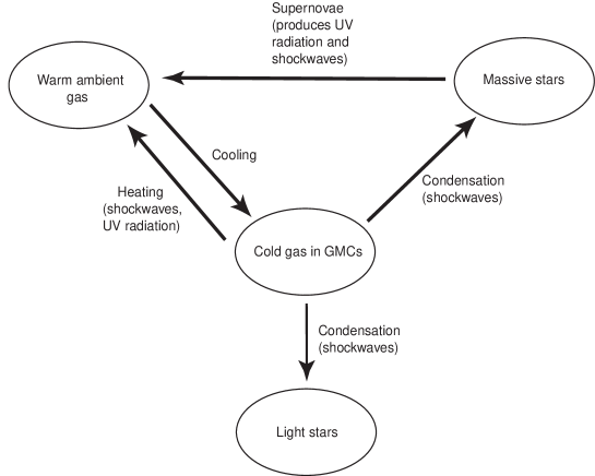
FIG. 1.: Diagram indicating matter flows in galactic disks, along with their catalysts.

TABLE I.: Description of the various components of the model; in the numerical simulation, these are all functions of radius, angle and time.

Variable	Description
$c$	Cold gas in GMCs
$g$	Warm, ambient gas
$s$	Massive stars
$d$	Light stars
$r$	Density of UV radiation
$h$	Density of shockwaves from supernovae

TABLE II.: Parameters of the model; the rationale behind these choices is given in [7].

Parameter	Value	Description
$\alpha_{1}$	0.1 - 1	Rate of GMC increase via cooling
$\alpha_{2}$	$5\times 10^{-2}-10^{-4}$	Rate of GMC decrease via heating
$\beta_{1}$	0.1 - 10	GMC destruction rate by shockwaves
$\beta_{2}$	0.02 - 2	Massive star production rate by shockwaves
$\beta_{3}$	0.08 - 8	Light star production rate by shockwaves
$\gamma$	$3\times 10^{-2}-5$	GMC destruction rate by massive star heating
$\epsilon_{1}$	0.2 - 2	Destruction rate of clouds via collisions
$\epsilon_{2}$	0.18 - 1.8	Formation rate of warm gas from cloud-cloud collisions
$\epsilon_{3}$	0.004 - 0.04	Formation rate of massive stars from cloud-cloud collisions
$\epsilon_{4}$	0.02 - 0.2	Formation rate of massive stars from cloud-cloud collisions
$\eta_{1}$	10	Production rate of UV radiation by SNe
$\eta_{2}$	0.02 - 1	Production rate of shockwaves of SNe
$\phi_{1}$	0.6	Average optical depth of UV radiation
$\phi_{2}$	0.4	Average “shock depth” of SNe shockwaves
$\delta$	0.001 - 0.003	Rate of warm gas accretion onto the galactic disk

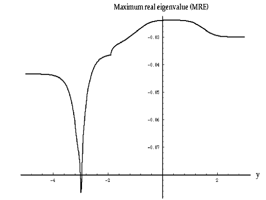
FIG. 2.: A graph of the maximum real eigenvalue (MRE) versus $y=\log({\bf k})$.

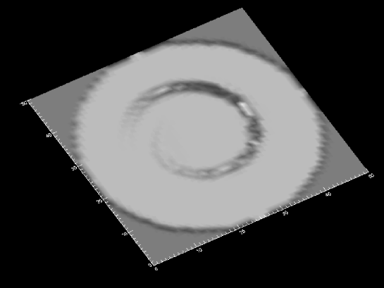
FIG. 3.: A surface plot of the (light) stars component at $250$ million years, about one revolution of the galactic disk. Note a spiral arm forming and developing.

REFERENCES

- [1] J. Binney and S. Tremaine, Galactic Dynamics (Princeton University, Princeton, 1987)
- [2] C. C. Lin and F. Shu, Astrophys. J. 236, 646 (1964); C. C. Lin and F. Shu, Proc. Nat. Acad. Sci. USA 55, 229 (1966)
- [3] D. M. Elmegreen and B. G. Elmegreen, Mon. Not. R. Astron. Soc. 201, 1021 (1982)
- [4] D. M. Elmegreen and B. G. Elmegreen, Astrophys. J. Suppl. Ser. 79, 37 (1984); D. M. Elmegreen and B. G. Elmegreen, Astrophys. J. 320, 183 (1987)
- [5] S. N. Shore and F. Ferrini, Fundamentals of Cosmic Physics 16, 1 (1995)
- [6] H. Gerola and P. E. Seiden, Astrophys. J. 223, 129 (1978); H. Gerola, P. E. Seiden, and L. S. Schulman, Astrophys. J. 232, 702 (1979); P. E. Seiden and H. Gerola, Fundamentals of Cosmic Physics 7, 241 (1982); L. S. Schulman and P. E. Seiden, Science 233, 425 (1986); L. S. Schulman and P. E. Seiden, Adv. Phys. 39, 1 (1990); Schulman, L. S. 1993, in Cellular Automata: Prospects in Astrophysical Applications, edited by A. Lejeune and J. Perdang (World Scientific, Singapore, 1993), p. 294
- [7] D. Cartin, Ph.D. thesis, the Pennsylvania State University, 2000
- [8] A. Freund, preprint arXiv:astro-ph/9705143, 1997; L. Smolin, preprint arXiv:astro-ph/9612033, 1996
- [9] E. Ben-Jacob, Contemporary Physics 33, 247 (1993); E. Ben-Jacob, Contemporary Physics 38, 205 (1997)
- [10] S. Kauffman, The Origin of Order (Oxford University, Oxford, 1993); H. Meinhardt, Models of Biological Pattern Formation (Academic, New York, 1992)
- [11] A. Zaikin and A. Zhabotinsky, Nature 225, 535 (1978)
- [12] E. Ben-Jacob and P. Garik, Nature, 323, 523 (1990); J. S. Langer, Science 243, 1150 (1989)
- [13] P. Bak, C. Tang, and K. Wiesenfeld, Phys. Rev. Lett. 59, 381 (1987); P. Bak, C. Tang, and K. Wiesenfeld, Phys. Rev. A 38, 364 (1988)
- [14] A. Sandage, Astron. Astrophys. 161, 89 (1986)
- [15] A. Burkert and G. Hensler, Astrophys. Space Sci. 171, 149 (1990); D. P. Cox and J. Franco, Astrophys. J. 273, 243 (1983); J. Franco and S. N. Shore, Astrophys. J.285, 813 (1984); A. Dopita, Astrophys. J. 295, L5 (1985); J. Silk and R. F. G. Wyse, Astrophys. J. 296, L1 (1985); C. F. McKee, Astrophys. J. 345, 782 (1989)
- [16] A. Parravano, Astron. Astrophys. 205, 71 (1988); A. Parravano, Astrophys. J. 347, 812 (1989); A. Parravano, P. Rosenzweig, and M. Teran, Astrophys. J. 350, 100 (1990); J. Mantilla Ch., and A. Parravano, Astrophys. J. 250, 70 (1991)
- [17] A. Turing, Philos. Trans. R. Soc. London 237B, 37 (1952)
- [18] F. C. Adams, S. Lizano, and F. H. Shu, Annu. Rev. Astron. Astrophys. 25, 23 (1987); C. J. Lada and F. H. Shu, Science 248, 564 (1990)
- [19] R. B. Larson, in Star Formation in Stellar Systems (III Canary Islands Winter School of Astrophysics), edited by G. Tenorio-Tagle, M. Prieto, and F. Sánchez (Cambridge University, Cambridge, 1992)
- [20] G. Tenorio-Tagle, in Regions of Recent Star Formation, edited by R. Roger and P. Dewdney (Reidel, Dordrecht, 1982)
- [21] P. Grindrod, Patterns and Waves: The Theory and Applications of Reaction-Diffusion Equations (Clarendon, Oxford, 1991); J. D. Murray, Mathematical Biology (Springer-Verlag, Berlin, 1993)
- [22] B. G. Elmegreen and M. Thomasson, Astron. Astrophys. 272, 37 (1992)
- [23] T. Neukirch and J. V. Feitzinger, Mon. Not. R. Astron. Soc. 235, 1343 (1988)