Are There Blue, Massive E/S0s at $z<1$ ?: Kinematics of Blue Spheroidal Galaxy Candidates

Abstract

Several recent studies find that 10 – 50% of morphologically selected field early-type galaxies at redshifts $z\lesssim 1$ have blue colors indicative of recent star formation. Such “blue spheroids” might be massive early-type galaxies with active star formation, perhaps induced by recent merger events. Alternatively, they could be starbursting, low-mass spheroids. To distinguish between these two choices, we have selected 10 “Blue Spheroid Candidates” (hereafter, BSCs) from a quantitatively selected E/S0 sample to study their properties, including kinematics from Keck spectra obtained as part of the DEEP Groth Strip Survey (GSS). Most BSCs (70%) turn out to belong to two broad categories, while the remaining objects are likely to be misclassified objects. Type-1 BSCs have underlying red stellar components with bluer inner components. Type-2 BSCs do not show an obvious sign of the underlying red stellar component, and their overall colors are quite blue ($(U-B)_{rest}<0$). Both Type-1 and Type-2 BSCs have internal velocity dispersions measured from emission lines $\sigma\lesssim 80$ km sec^-1 and estimated dynamical masses of only a few $\times 10^{10}M_{\sun}$ or less. For Type-1 BSCs, we estimate $\sigma$ of the red component using the fundamental plane relation of distant field absorption-line galaxies and find that these $\sigma$ estimates are similar to the $\sigma$ measured from emission lines. Overall, we conclude that our Type-1 and Type-2 BSCs are more likely to be star-forming low mass spheroids than star-forming, massive, early-type galaxies.

1. Introduction

When two gaseous galaxies merge, the gas sinks towards the center of the merger product, creating an intense burst of new stars, and the merger product has the surface brightness profile dominated by the $r^{1/4}$ law (e.g., Mihos & Hernquist 1994). Thus, the detection of many smooth, highly-concentrated, blue star-forming galaxies would provide strong support for the formation of early-type galaxies via mergers at $z<1$, as predicted by some hierarchical merger models (e.g., Baugh et al. 1996; Kauffmann et al. 1996).

Recently, several groups have identified blue galaxies at $z\lesssim 1$ that appear to be early-type galaxies such as E or S0s (Im et al. 2001; Menanteau et al. 1999; Schade et al. 1999; Abraham et al. 1999; Franceschini et al. 1998). Their surface brightness profiles show a significant $r^{1/4}$ component typical of nearby E and S0 galaxies, typically with bulge-to-total light ratios ($B/T$) greater than 0.4 (Im et al. 2001). Some of these galaxies are found to have [OII] emission lines, indicative of recent star formation (Koo et al. 1996; Schade et al. 1999). Also, others find younger, blue stellar components on top of underlying old, red stellar populations (Menanteau et al. 2000; Abraham et al. 1999). These morphological features, as well as their blue colors and the rather high luminosities of at least some of the blue spheroidal galaxies, suggest that they may be direct progenitors of the present-day typical, massive early-type galaxies ($>10^{11}M_{\sun}$ or $\sigma>150$ km/sec) which are undergoing strong star formation after merging.

The blue spheroidal galaxies, however, could instead be low-mass, starbursting dwarf galaxies such as dwarf ellipticals/spheroids (hereafter, dE following Mihalas & Binney 1981; e.g., Im et al. 1995a, 1995b; Babul & Ferguson 1996; Driver et al. 1996). The strong star formation activity at the center might create excess light over the exponential surface brightness profile commonly found in dwarf spheroids (Lin & Faber 1983; Gallagher & Wyse 1994), which could be interpreted as a significant bulge component. In fact, some blue spheroidal galaxies resemble distant compact galaxies (CGs; Koo et al. 1994, 1996; Guzmán et al. 1996, 1997, 1998; Phillips et al. 1997). The previous works on CGs suggest that at least some CGs are likely to be progenitors of low-mass spheroids ($\lesssim 10^{10}\,M_{\sun}$) today.

As a part of the DEEP Groth Strip Survey (GSS; Vogt et al. 2001a; Koo et al. 1996), we have identified 10 BSCs from HST images, and we have measured their emission line widths to obtain mass estimates. In this paper, we present evidence that, based on their kinematic and structural properties, the majority of BSCs are likely to be low-mass spheroidal galaxies undergoing strong starbursts, rather than massive star-forming E/S0s. Throughout the paper, the rest-frame quantities and model predictions are calculated assuming $\Omega_{m}=0.2$, $\Lambda=0$ and $h=0.7$ for the cosmological parameters, where the Hubble constant is normalized as $h=H_{0}/100~{}$km/sec.

2. Data

2.1. Sample

The BSCs are drawn from a set of 28 contiguous HST WFPC2 fields, the so called “Groth Strip” (Groth et al. 1994; Rhodes et al. 2000). A significant portion of the Groth strip was spectroscopically observed with the Keck 10-m telescope by the Deep Extragalactic Evolutionary Probe (DEEP; Koo et al. 1996; Vogt et al. 2001a; Simard et al. 2001; Phillips et al. 2001).

A combination of HST images and Keck spectra enables us to select BSCs as described below. We emphasize that our selection criteria for BSCs are quite different from those of the CGs in Phillips et al. (1997) and Guzḿan et al. (1997), and that our goal is to select galaxies which morphologically resemble local Es and S0s but with blue colors.

The first step in our procedure is to fit each HST galaxy image using the 2-dimensional bulge+disk surface brightness fitting algorithm GIM2D (Simard et al. 1999, 2001; Marleau & Simard 1998). The main purpose of fitting HST galaxy images with GIM2D is to derive structural and morphological parameters that can be used for quantitative selection of E/S0 galaxies (Im et al. 2001). The surface brightness profile of the bulge component is fitted with either a de Vaucouleurs (or $r^{1/4}$) profile or an exponential profile. The de Vaucouleurs profile is known to fit the surface brightness profile of ellipticals and bulges of luminous spiral galaxies (de Vaucouleurs 1948). Bulges of less luminous, late-type spirals are known to be fitted well with an exponential profile (e.g., Andredakis & Sanders 1994; de Jong 1996). For the component fitted as a bulge, we will use the term “photo-bulge”, since this component is mathematically defined by the surface photometry, though in some cases may not correspond to physically-defined “bulges” of nearby galaxies in terms of stellar population and kinematics. For the sample selection of BSCs, we will only use a deVaucouleurs profile for the photo-bulge component. The surface brightness profile of the disk component is fitted with an exponential profile, which is known to fit the SB of disks of spiral galaxies. In analogy to the photo-bulges, we will use the term “photo-disk” for this component. GIM2D measures model-fit structural parameters which include the total magnitude; bulge-to-total light ratio ($B/T$); disk scale length ($r_{d}$); bulge effective radius ($r_{e}$); galaxy half-light radius ($r_{hl}$); position angles and ellipticities for both the bulge and disk components, and errors associated with each quantity. Centers of both the photo-bulge and photo-disk components are assumed to be the same, and fitted along with the other structural parameters. This procedure of surface brightness fitting is similar to that of Ratnatunga, Griffiths, and Ostrander (1999), and Schade et al. (1995). GIM2D searches for a parameter set which gives the maximum likelihood value using Monte-Carlo sampling of the parameter space. Then, GIM2D Monte-Carlo samples the region around the maximum likelihood, and the median value of each of the parameters is adopted as the model-fit parameter; the errors are estimated at the 68% confidence level of the statistical distribution of the sampled parameter sets (Simard et al. 2001). The errors may be underestimated for two reasons: (1) PSF modeling errors are not included; (2) the sky levels are not fitted along with other parameters, thus the confidence intervals do not include errors on the sky level estimate. Our tests with simulations show, however, that these effects do not severely underestimate errors (see Simard et al. 2001). The assumed luminosity profiles can also affect the output parameters (see section 3.2). In general, $V$ and $I$ band images are fitted with GIM2D separately, which we call as “separate fit”, as opposed to “simultaneous fit” where $V$ and $I$ band images are fitted simultaneously to provide better constraints on the model-fit parameters such as $V-I$ (see section 3.2).

In the next step, early-type galaxy candidates are selected based on two quantitative morphological parameters, the bulge-to-total light ratio ($B/T$) and the residual parameter ($R$), which are derived from GIM2D using the “separate” fits. We use the “separate” fits for the sample selection since our early-type galaxy candidates come from the early-type galaxy sample of Im et al. (2001), which is based on the “separate” fit. The quantity $B/T$ measures the ratio of the luminosity in the photo-bulge component to the total luminosity contained in both photo-bulge and photo-disk components. Thus, the $B/T$ describes how prominent the photo-bulge component is, and typical values are $B/T>0.5$ and $B/T>0.3$ for visually classified local Es and S0s, respectively (Im et al. 2001; Kent 1985; Scorza et al. 1998). Note that the $B/T$ cut alone is not very effective at isolating E/S0s. Some late-type galaxies have $B/T>0.3$ – 0.4, and about 30% of objects selected with the $B/T>0.3$ – 0.4 cut are indeed non-E/S0 galaxies (Im et al. 2001; Kent 1985). For that reason, we use another parameter – the residual parameter ($R$) – to exclude non-E/S0 galaxies with large $B/T$ values.

The residual parameter $R$ describes how symmetric and prominent the morphological substructures are (such as spiral arms and HII regions). Smooth-looking, symmetric galaxies like E/S0s generally have $R\lesssim 0.08$. For a detailed description of the $R$ parameter, see Im et al. (2001) and Schade et al. (1995). Im et al. (2001) select “Quantitatively-Selected E/S0s” (hereafter, QS-E/S0s) with the criteria $B/T>0.4$ and $R\lesssim 0.05$ – $0.08$, depending on the size and apparent magnitude of the object. Tests on simulated local galaxy images show that these criteria select E/S0s well (Im et al. 2001). The $R$ cut varies as follows: $R\leq 0.08$ when $I<21.0$, $R\leq 0.06$ when $21.0<I<21.5$, and $R\leq 0.05$ when $21.5<I<22$. ($I$-band magnitude is defined as the total model magnitude derived from the surface brightness fit; note that this total magnitude will be used throughout the paper, unless noted otherwise). The $R$ cuts are chosen to minimize the contamination of the QS-E/S0 sample by late-type galaxies when the S/N is low ($S/N\lesssim 50$). We use the same criteria to choose QS-E/S0s in this paper, which are identical to QS-E/S0s in Im et al. (2001).

As a next step, the spectroscopic redshift-color diagram is used to identify unusually blue QS-E/S0s as BSCs, where the color ($V-I$) is also derived from the model total magnitudes. Fig. 1 shows the $(V-I)$ vs. spectroscopic redshift diagram of a magnitude limited sample ($I<22$) of 262 galaxies in the Groth strip. Note that the identification of spectroscopic redshifts is virtually complete to this magnitude limit for the GSS (Phillips et al. 2001). Also shown in Fig. 1 are lines of plausible color ranges for passively evolving, old stellar populations computed with the 1996 version of the spectral synthesis model of Bruzual & Charlot (1993; hereafter, GISSEL96) – the upper dashed line is created by assuming a 0.1 Gyr burst with 250% solar metallicity, Salpeter IMF, and formation redshift $z_{for}=11$. The lower line assumes the same model with lower metallicity (40% solar). To allow for magnitude errors, we add/subtract 0.15 magnitude in $(V-I)$ color to the upper/lower lines. Im et al. (2001) find that most QS-E/S0s (marked with squares) form a red envelope in the $(V-I)$ vs. redshift diagram. However, six out of 44 QS-E/S0s (marked with thick triangles) have colors that are bluer than the expected color range of the passive evolution model; we call these QS-E/S0s “good” BSCs.

In addition to these “good” BSCs, we have examined images of galaxies that would have been selected as BSCs if the morphological selection criteria were slightly less restrictive ($B/T>0.35$ or $R\lesssim 0.09$). This visual inspection reveals 4 additional candidates, and we call them “possible” BSCs (thin triangles in Fig. 1). Fig. 2 shows $I$-band images of the 6 “good” BSCs and 4 “possible” BSCs. By constructing an azimuthally-averaged surface-brightness (SB) profile using ellipsoidal apertures and plotting it along the major axis, we confirm that our BSCs show surface brightness profiles which differ significantly from a simple exponential law, but that are well fitted by the addition of a significant photo-bulge component. This and other important points regarding the colors and structures of the underlying stellar populations are discussed in more detail in Section 3.2.

Fig. 3 shows the spectroscopic redshifts vs. $I$ for “good” BSCs (thick triangles) and “possible” BSCs (thin triangles), compared with red QS-E/S0s (squares) and all other types of galaxies (dots) in the GSS. Below $z=0.5$, there tends to be a dichotomy in the sense that red QS-E/S0s are intrinsically bright while BSCs are faint. Their faint apparent magnitudes suggest that low-$z$ BSCs are unlikely to evolve into massive E/S0s today. In contrast, above $z=0.5$, BSCs approach $L^{*}$ in luminosity. However, the apparent brightness of $z>0.5$ BSCs does not necessarily mean that they will evolve into the present-day $L^{*}$ E/S0s, as the luminosity dimming for these galaxies may be more significant than that of the old stellar populations which are assumed in lines of Fig.3 – thus, these $L\sim L^{*}$ high-$z$ BSCs may fade significantly into low-luminosity systems today.

To improve constraints on the local counterparts of BSCs, we need to study quantities which are independent of the luminosity evolution and are more direct tracers of the mass, e.g., the internal velocity dispersion $\sigma$. The next section describes our measurements of the internal velocity dispersion, $\sigma$, for these BSCs.

2.2. Spectroscopic observations and line width measurements

Spectra of BSCs were obtained as a part of the DEEP survey during the 1996-1999 Keck observing runs (Phillips et al. 2001) using the Low Resolution Imaging Spectrograph (LRIS; Oke et al. 1995). A 900 lines/mm grating was used to cover the blue part of the spectrum ($\sim 5000$ – $6500$ Å) and a 600 lines/mm grating was used for the red part ($\sim 6500$ – $8500$ Å); typical exposures were $\sim$ 1 hour with each grating. The spectral resolution (FWHM$\sim$ 2 Å  and 4 Å  for the blue and red parts, respectively, or $\Delta\sigma\sim 80$ km sec^-1 with $\Delta\sigma$ defined as $\sigma$ of the instrumental resolution) allows us to measure $\sigma$ as low as $\sim$ 30 km  sec^-1. For one BSC (092_1339), we also obtained a 15-min high resolution spectrum ($\Delta\sigma\sim 17$ km sec^-1) using the Echellette Spectroscopic Imager (ESI; Sheinis, et al. 2000) during May, 2000, at Keck.

To measure the line widths, we fit Gaussian profiles to strong S/N emission lines following the method described in Phillips et al. (1997) and Guzmán et al. (1997). For the [OII] doublet at 3727 Å, we used a double Gaussian profile with a fixed $\Delta\lambda$ between both peaks. Each velocity width was corrected for the instrumental resolution. Finally, we take the variance-weighted mean value of the velocity widths measured from different lines as our adopted $\sigma$.

Estimating true errors of velocity widths is not a trivial task, as uncertainties in velocity widths include various factors beyond the formal measurement error. This is particularly true in estimating the instrumental correction, which varies with galaxy extent, seeing disk size, and misalignment of the target with the slit. In addition, the non-uniform distribution of the emission and non-Gaussian velocity profiles contribute to the intrinsic error. Simulations with realistic parameters indicate a “robust” velocity error of about one-third the instrumental line width, a value which is supported by repeat observations of the same objects, and by line width measurements using different algorithms (Phillips et al. 2001; Guzmán et al. 1997). For LRIS, this corresponds to $\sim 30$ km sec^-1 depending on the line and redshift of the object. Hence, we adopt 1-$\sigma$ error, $\delta\sigma=30$ km sec^-1, as a good (conservative) error estimate (see Phillips et al. 2001 for a full discussion). For the ESI data, we adopt $\delta\sigma=6$ km sec^-1, which is simply one-third of the ESI resolution. The $\sigma$ values can be found in Table 1.

In Fig. 4, we show spectra centered on the [OII] emission line for 3 representative BSCs. Interestingly, an inspection of the 2-D spectra of two “good” BSCs (092_4957 and 294_2078) show tilted emission lines, indicating that they are rotating objects (e.g, disks). One “good” BSC (212_1030) has a weak [OII] emission line, but it is not clear whether the emission line comes from the object itself or from its blue neighbors, at least one of which is at the same redshift. Finally, one “possible” BSC (082_5252) has a redshift taken from the literature (Lilly et al. 1995), so we do not have a measured $\sigma$ for this object.

3. Results

In this section, we present our two main findings about BSCs. In section 3.1, we will show that the dynamical masses of BSCs are similar to those of nearby low-mass spheroidal galaxies, assuming that the dynamical mass estimated from the emission line widths is not severely underestimated (less than a factor of $\sim 2$). Then, in section 3.2, we show that 5 – 6 out of 10 BSCs seem to have an underlying old stellar population, and that their blue overall colors originate from localized regions containing young stars. In the same section, we also discuss a plausible shape of the surface brightness profile as a means to explore the structure of the underlying stellar population.

3.1. Mass of BSCs

In Table 1, we present the basic data for BSCs. Note that structural parameter values in Table 1 come from the “separate” fit described in Section 2. We estimate the dynamical mass using the virial theorem for spherical $r^{1/4}$ law systems (Poveda 1958; Young 1976; Illingworth 1976):

$$M_{dyn}\simeq 3\sigma_{3D}^{2}r_{1/2}/G,$$

where $\sigma_{3D}$ is the central velocity dispersion of the system in real 3-D space, $r_{1/2}$ is the projected half-mass radius, and $G$ is the gravitational constant. We assume that stellar mass traces light, i.e., $r_{1/2}\simeq r_{hl,cir}$, where $r_{hl,cir}$ is the projected circular aperture half-light radius of the stellar system in Table 1 (roughly equal to the major-axis half light radius, if the ellipticity, $e$, is small). Note that we use $r_{hl,cir}$, instead of $r_{hl,maj}$ which is defined along the major axis and given as a default output from GIM2D, in order to facilitate the comparison with local samples for which $r_{hl,maj}$ is not readily available. The line of sight velocity dispersion $\sigma$ would be $\sigma_{3D}/\sqrt{3}$ in an isotropic velocity field. Therefore, the total dynamical mass of the system is roughly,

$$M_{dyn}\simeq 9\,\sigma^{2}\,r_{hl,cir}/G.$$ (1)

This formula is similar to that adopted by Phillips et al. (1997).

Fig. 5, shows measured $\sigma$ vs. $r_{hl,cir}$ for all BSCs (triangles). Also plotted in Fig. 5 are regions occupied by different galaxy types at $z=0$, taken from Phillips et al. (1997) and Guzmán et al. (1998). Dashed lines are drawn to indicate constant mass. In the same plot, squares indicate $r_{hl,cir}$ vs. $\sigma$ of distant, red, QS-E/S0s ($I<22$) with spectroscopic redshifts in Im et al. (2001). For the Im et al. (2001) sample, we use measured $\sigma_{abs}$ when they are available (Gebhardt et al. 2001), and $\sigma_{FP}$ (see Section 4.1) otherwise. Fig. 5 shows that no BSCs resemble present-day, massive, early-type galaxies or distant red, QS-E/S0s. The majority of BSCs (5 out of 9) lie within or on the border of the polygon for local dEs, suggesting a possible link. BSCs have $\sigma\lesssim 80$ km/sec and $M\lesssim 10^{10}M_{\sun}$. Typical, massive, luminous E/S0s ($L\gtrsim L^{*}$) have $\sigma\gtrsim$ 150 km/sec and $M\gtrsim 10^{11}M_{\sun}$. Thus, BSCs are not likely to evolve into massive E/S0s today under the assumption that the measured $\sigma$ reflect the dynamical galaxy mass. Studies exist which support this assumption (e.g., Telles & Terlevich 1993; Kobulnicky & Gebhardt 2000 and references therein), but future studies with more extended samples may be needed to establish the link between $\sigma$ measured from emission lines (hereafter, $\sigma_{em}$) and dynamical mass of galaxies – these points are discussed in section 4.1, where we argue that our conclusion here is not likely to change even if our $\sigma_{em}$ values somewhat underestimate $M_{dyn}$.

Note that CGs studied by Phillips et al. (1997) and Guzmán et al. (1996) also lie in a similar region where BSCs are (see Fig.9 of Phillips et al. 1997). From the $B/T$ and $R$ values which we derived separately for CGs, we find that roughly 10% of CGs at $I<22$ in the Phillips et al. (1997) and Guzmán et al. (1996) sample can be classified as BSCs. The number of BSCs found in the CG sample per WFPC2 frame (0.25 per frame) matches well with the number of BSCs found here. Conversely, we can apply the selection criteria of CGs in Phillips et al. (1997) to our sample, and we find that 8 out of 10 BSCs are CGs. Thus, we conclude that most BSCs belong to a subset of CGs that are smooth and photo-bulge-dominated.

A more detailed description of each BSC in Fig.5 is presented below. One BSC (062_6465; #7) lies in the region of Irr galaxies, but not too far from the locus of dEs. Two BSCs (294_2078, 212_1030; #6 and #5 respectively) are found in the spiral galaxy polygon. As noted above, the spectrum of one of them (294_2078) shows tilted emission lines indicative of a rotating system. Furthermore, the measured $B/T$ value has a relatively large error (e.g., $B/T=0.59^{+0.07}_{-0.14}$ from Table 1), and this galaxy is a highly-inclined system. Thus, BSC 294_2078 is probably an early-type spiral with a significant disk component or a later-type galaxy. BSC 212_1030 is an absorption-line object with a possible weak [OII] emission line. The blue companion on the left in Fig. 2 has a redshift virtually identical to 212_1030 ($z=0.88$), and is possibly physically associated. The projected separation between both objects is $\sim$ 1.2 arcsec (6 $h^{-1}$ kpc). The blue galaxies on the right are foreground objects with redshifts $z\simeq 0.24$, much lower than the redshift of 212_1030, and so are not physically associated. Unfortunately, the spectrum of 212_1030 is too noisy to measure the absorption-line velocity width. Its nuclear color measured with an aperture size of 0.5 arcsec is $V-I=1.9$, much redder than the total color $V-I=1.58$ from the model fit. We also note that model-fit colors of this object using different procedures are $V-I\simeq 1.7$ – $1.8$. Therefore, we suspect that the model-fit color of 212_1030 is somehow contaminated by its blue neighbors, and that this object is not a genuine BSC, but rather is more likely to be a normal, red, early-type galaxy.

Another BSC (092_4957; #2), which lies close to the border of dEs and spirals, has a rotation curve with an inclination-corrected rotational velocity, $V_{max}\simeq 130$ km/sec (Vogt 2000, private communication). The velocity width of $\sigma\simeq 60$ km sec^-1, is in agreement with the $V_{max}$ value considering the conversion factor of $\frac{1.81}{sin(inc)}$ in $V_{max}\simeq\frac{1.81}{sin(inc)}\times\sigma_{[OII]}$, which typically amounts to $\sim 2$ (Kobulnicky & Gebhardt 2000). The disk component of this object is found to lie on the local TF relation, a strong indication that this object may be a relatively low-mass spiral galaxy (Vogt et al. 2001b).

3.2. Underlying stellar population

The accretion of gas-rich satellite galaxies or gas infall toward the centers of E/S0 galaxies may provide fuel which will trigger intense star formation. Young stars in the satellite galaxies can also fall into the centers. The existence of relatively-young stellar populations among local E/S0 galaxies suggests that such a sprinkling of young stars over an old, underlying, stellar population has occurred (e.g., Charlot & Silk 1994; Trager et al. 2000). If BSCs are old galaxies sprinkled with young stars near their center, we should find that the outskirts are red, while the inner parts are blue. Fig. 6 shows the rest-frame $U-B$ color gradient of BSCs along their major axis out to $\sim 3~{}r_{hl,maj}$, as well as a 2-dimensional color map. To construct the 2-D color gradient plot, we used the IRAF task, “ellipse” with a fixed object center, an ellipticity and a position angle which all correspond to the values derived for the photo-bulge component of the “separate” 2-D fit. Background sky levels were estimated using a region which is at least 5 pixels away from the object pixels . In the process, observed $V-I$ values are converted to the rest-frame $U-B$ using the empirical $K$-correction which is presented in Gebhardt et al. (2001).

To construct the 2-D color map, we used the following procedure: First, both the $V$- and $I$-band images of each object are background subtracted, and smoothed with Gaussian filter with $\sigma=1$. This smoothing of the image with the Gaussian filter is necessary to enhance the global color gradients. In the next step, each pixel value is converted into magnitude units. Then, the $I$-band image is subtracted from the $V$-band image to produce a color image. Finally, the $V-I$ values are converted to the rest-frame $U-B$ color. The expected $U-B$ values for a passively evolving stellar population after a 0.1 Gyr burst are $U-B=0.1\sim 0.2$ at the age of 1 Gyr and $U-B=0.2\sim 0.5$ at the age of 5 Gyr, for the assumed metallicities of 40% and 100% solar values, respectively (GISSEL96).

Fig. 6 suggests that there are three categories of BSCs, as described below.

Type-1: Five, possibly six, out of the 10 BSCs show a tendency to have blue inner regions and red outer regions, suggesting that these BSCs have underlying old stellar populations ($092\_1339,103\_6061,172\_5049,062\_6465,082\_5252$, and possibly $153\_6056$). Red outer regions are as red as the expected colors of passively-evolving stellar populations ($U-B\simeq 0.1\sim 0.5$), and redder than colors of local Sbc’s ($U-B\simeq 0.0$). Thus, these BSCs might be old galaxies with star formation occurring more actively near their centers; similar objects have been discussed in Guzmán et al. (1998), Abraham et al. (1999) and Menanteau et al. (2000). Note that Jansen et al. (2000) find that 50% of the local, low-luminosity galaxies have the bluest colors at their centers – Type-1 BSCs may be comparable to such local low-luminosity galaxies.

Type-2: One, or possibly two BSCs ($273\_4427$ and possibly 153_6056) do not have a significantly redder outer region, and their overall colors are bluer than Sbc’s.

Misclassifications: Two BSCs have red cores and blue outer regions ($092\_4957$ and $294\_2078$). Both have tilted emission lines, indicative of rotation. Their rotation signature, as well as the overall structural and color gradient appearance suggest that they are more likely to be late-type galaxies rather than genuine BSCs. The remaining BSC ($212\_1030$) seems to be an early-type galaxy with a red color similar to that of local early-type galaxies.

Further evidence for the existence of red outer regions for Type-1 BSCs comes from the 2-dimensional bulge+disk SB profile fits. These provide the structural parameters and colors of photo-bulge and photo-disk components, which can be compared with the results obtained from the color gradient analysis. Since we are interested in obtaining well-constrained colors and structural parameters for each component, we use the “simultaneous” fitting method, i.e., where we fit the $I$-band and $V$-band images of each BSC simultaneously, allowing only the total flux, $B/T$, and the background correction to be different in each band (Simard et al. 2001; Koo et al. 2001).

To test the robustness of our results to the assumptions for the adopted SB profiles, we tried two kinds of SB models – the “$r^{1/4}$ + disk model” which uses a $r^{1/4}$ law profile for the photo-bulge and an exponential profile for the photo-disk, and the “double exponential model” which adopts exponential profiles for both photo-bulge and photo-disk components. Note that the derived structural parameter values from these “simultaneous” fits (Tables 2 and 3) can be slightly different from the values derived from the “separate” fits described in section 2, which is used for the sample selection (Table 1).

Fig. 7 shows the azimuthally averaged major axis surface brightness profile of BSCs (points) obtained from the aperture photometry, together with the best-fit model profile from GIM2D (solid line) which is composed of a photo-disk (dotted line) and a photo-bulge (dashed line). Fig. 7 shows that the surface brightness profiles cannot be fitted well with a single exponential profile – a significant second component is needed to fit their SB profile. In Tables 2 and 3, we list the GIM2D parameters from the “simultaneous” $r^{1/4}$+disk and double exponential model fits, respectively. The important quantity in Tables 2 and 3 is the color of the more extended component, i.e., a component whose half-light radius is the larger of the two ($r_{hl,maj}=r_{e,maj}$ for a $r^{1/4}$ component, and $r_{hl,maj}=1.68\,r_{d,maj}$ for an exponential component). Regardless of the assumed model SB profile, the extended components (typically, photo-bulge) of three Type-1 “good” BSCs indeed have a color redder than typical Sbcs ($U-B\simeq 0$) or as red as the expected colors of passively-evolving E/S0s ($U-B\gtrsim 0.1$), providing an independent confirmation for the existence of a red underlying stellar population in these BSCs. For the three remaining “possible” BSCs, the 2-D profile fits are less conclusive. Some redder components are not more extended. Nevertheless, even for such cases, the redder and bluer components have comparable $r_{hl,maj}$. We will use the term “underlying red stellar component” or “underlying red component” to describe the extended red component which seems to exist in Type-1 BSCs.

In principle, the shape of the surface brightness profile of the underlying red stellar population can tell us about the likely local counterparts of these BSCs. If they are like massive E/S0s, the underlying stellar population will be distributed following the $r^{1/4}$ law profile. On the other hand, the underlying red component will show an exponential SB profile, if BSCs are more likely progenitors of less massive spheroids. Unfortunately, we find that the difference in reduced $\chi^{2}$ values from both fitting models is small ($\Delta\chi^{2}\lesssim 0.01$), meaning that the $r^{1/4}$+disk model and the double exponential model are almost equally good. Thus, the current data do not constrain the likely local counterpart of the BSCs in terms of the surface brightness profile. Any underlying old stellar population will stand out more clearly in the near-infrared (NIR; e.g., Hammer et al. 2001); thus an analysis of high-resolution NIR images should offer more insights toward the characteristic SB profile and the mass content of the red component.

4. Discussion

This section provides detailed discussions on our findings. In section 4.1, we discuss the robustness of the use of emission line widths for mass estimates. Section 4.2 shows detailed comparison of our BSCs vs. other BSCs in the literature, and section 4.3 discusses BSCs in the Hubble Deep Field. A rough estimate of the number density of BSCs is given in section 4.4, and section 4.5 discusses BSCs and their interaction with close neighbors.

4.1. Mass of the underlying stellar population

In the previous section, we found that 5 or 6 Type-1 BSCs in our sample appear to have an underlying, extended, red stellar component ($U-B>0.0$) and a bluer core from where most of the flux in emission lines may originate. When the star formation is very localized, the line width from emission lines can be much narrower than a more global velocity dispersion. It is thus reasonable to ask how well the velocity dispersion measured from the emission lines really represents the velocity dispersion of the entire galaxy, especially for Type-1 BSCs.

One possible way to resolve this issue is to directly compare $\sigma_{em}$ with the observed absorption-line velocity dispersions ($\sigma_{abs}$) of underlying stellar populations. Kobulnicky & Gebhardt (2000) measure both $\sigma_{abs}$ and $\sigma_{em}$ for a sample of local galaxies of various morphological types, and find that $\sigma_{abs}$ and $\sigma_{em}$ correlate well. However, their sample does not contain E/S0 galaxies, and thus may not be directly applicable to BSCs. For a sample of nearby elliptical galaxies, Phillips et al. (1986) measured $\sigma_{em}$(core) from [NII]. We identify 21 ellipticals in Phillips et al. (1986) which overlap with the elliptical galaxy sample of Faber et al. (1989) for which $\sigma_{abs}$(core) is available. Here, we use the notation “(core)”, since both $\sigma_{em}$ and $\sigma_{abs}$ are measured within $r\lesssim 0.1\,r_{hl}$. The comparison between $\sigma_{abs}$(core) and $\sigma_{em}$(core) reveals that of these 21 massive ellipticals, all have $\sigma_{abs}$(core) $>130$ km sec^-1 and none have $\sigma_{em}$(core)$<100$ km sec^-1. Some ellipticals in Phillips et al. (1986) do have $\sigma_{em}$(core) $<$ 80 km sec^-1, but these galaxies are found to be rather less luminous systems ($M_{B}\lesssim-19.5$) and have [NII]$\lambda$6584/$H_{\alpha}$ ratios $\lesssim 0.2$, resembling HII galaxies. Some BSCs have $\sigma_{em}$ and $M_{B}$ values very similar to the local HII-like ellipticals. A weakness in this comparison is that $\sigma$ are measured only near the core in Phillips et al. (1986), while $\sigma_{em}$ of our BSCs are measured over a more extended region ($\sim r_{hl}$).

For distant early-type galaxies, Koo et al. (2001) discuss $\sigma_{em}$ vs $\sigma_{abs}$ of luminous bulges at $z\sim 0.8$. They find 5 luminous bulges for which $\sigma_{em}$ is measurable, and find a reasonable agreement between $\sigma_{em}$ and $\sigma_{abs}$. None of these five objects have $\sigma_{em}<100$ km sec^-1. We find a similar result for the E/S0 galaxy sample of Im et al. (2001), which contains at least 5 objects with both $\sigma_{abs}$ and $\sigma_{em}$.

We would like to emphasize that none of the luminous bulges or E/S0s in either the nearby or distant samples have $\sigma_{em}<$ 100 km sec^-1. The lack of massive local ellipticals with $\sigma_{em}<80$ km sec^-1 suggests that Type-1 or Type-2 BSCs are more likely to be low-mass ellipticals with intense star formation rather than massive E/S0s.

A more direct test would be to compare both $\sigma_{em}$ and $\sigma_{abs}$ of the underlying old stellar population of BSCs. Unfortunately, our BSCs are in general too faint to provide continuum spectra with enough S/N for the measurement of $\sigma_{abs}$. For this reason, we derive a limit on $\sigma_{abs}$ for only one object (103_6061) in our sample. Fig. 8 shows a continuum-divided, absorption-line spectrum of 103_6061, from which we obtain an upper limit $\sigma_{abs}<80$ km sec^-1. The observed spectrum is fitted with a model spectrum using a maximum-penalized likelihood method (Gebhardt et al. 2001; also see Saha & Williams 1994; Merritt 1997). The model spectrum is comprised of high-resolution, stellar templates which are convolved according to a given velocity dispersion and instrument resolution and are mixed with proper weights to provide the best match to the galaxy spectrum. For more details on the absorption line fitting method, see Gebhardt et al. (2001). Some absorption lines in this particular object are contaminated by emission lines (dotted line in Fig. 8), and we artificially remove these lines when fitting the spectrum. In the figure, Balmer emission lines seem narrower than the stellar absorption lines, but this is simply because stellar lines are intrinsically broader than the nebular emission lines in the absence of velocity fields. The upper limit on $\sigma_{abs}$ (80 km sec^-1) for 103_6061 is perfectly consistent with its $\sigma_{em}$ value of 61 km sec^-1, supporting the assumption that $\sigma_{em}$ reflects the galaxy mass, or at least that $\sigma_{em}$ does not severely underestimate the kinematics of the galaxy.

As an alternative check, we use the fundamental plane relation of field, early-type galaxies at $z\lesssim 1$ (Gebhardt et al. 2001) to estimate the velocity dispersion of the red, underlying components (hereafter, $\sigma_{FP}$). This approach assumes that BSCs with underlying red, stellar populations, as defined in the previous section, are early-type galaxies with a sprinkling of young stars at their center. The FP relation in Gebhardt et al. (2001) may be written as,

$$log_{10}(\sigma_{FP}{\rm(km\,s^{-1})})=0.8~{}[log_{10}(r_{hl,under}{\rm(kpc)})+0.32\langle SB_{hl,under}\rangle+9.062)],$$ (2)

where $r_{hl}$ has been replaced by $r_{hl,under}$, the circular aperture half-light radius of the underlying, red component. $SB_{hl,under}$ is the rest-frame $B$-band surface brightness within $r_{hl,under}$ of the same component corrected for the luminosity evolution derived in Gebhardt et al. (2001). Since there is uncertainty regarding the plausible surface brightness profile for BSCs, we use structural parameters from both the simultaneous $r^{1/4}$+disk fit (Table 2) and the double exponential fit (Table 3), and use them to derive independent $\sigma_{FP}$ values. The quantity $r_{hl,under}$ is derived as $r_{hl,under}=\sqrt{1-e_{b}}\times r_{e,\rm maj}$ from Table 2 when the underlying red component is fitted with a $r^{1/4}$ law. When the underlying red component is fitted with an exponential profile, we use $r_{hl,under}=1.68\,\sqrt{cos(inc)}\,r_{d,maj}$ from Table 2 or Table 3.

In Table 4, we compare these $\sigma_{FP}$ versus $\sigma_{em}$. Note that the numbers within parentheses are the values derived from a double exponential profile. First, we find that $\sigma_{FP}$ using the $r^{1/4}$+disk fit differ from $\sigma_{FP}$ derived using the double exponential fit. In many cases, the difference between two $\sigma_{FP}$ values is small ($\pm$10 – 20%), but in some cases, $\sigma_{FP}$ values from these different methods differ almost by a factor of two (172_5049 and 103_6061).

Second, the comparison between the $\sigma$ values shows that $\sigma_{em}$ values are similar to or smaller than $\sigma_{FP}$ by $20\pm 20$% on average. The derived ratio, $\frac{\sigma_{em}}{\sigma_{FP}}$, is consistent with similar values derived from the comparison of velocity widths measured in HI, optical emission lines, and optical absorption lines for local galaxies (Kobulnicky & Gebhardt 2000; Telles & Terlevich 1993; Rix et al. 1997). The amount of discrepancy is small enough to ensure that mass of BSCs in Table 1 should not be underestimated by more than a factor of $\sim$2. In Fig. 9, we show $r_{hl,under}$ vs. $\sigma_{FP}$ of BSCs in Table 4. Like Fig. 5, we also plot the same relation for distant, red, QS-E/S0s (squares). The diamonds show $r_{hl,under}$ vs $\sigma_{FP}$ for the $r^{1/4}$ + disk fit, and the stars indicate the same relation for the double exponential fit. Fig. 5 shows that BSCs still lie in the region which is populated by low-mass Es and dEs ($M_{dyn}<$ a few $\times 10^{10}\,M_{\odot}$) even though we use $\sigma_{FP}$. A possible exception is 092_1339 (#1), which may have a dynamical mass of $\sim 10^{11}\,M_{\odot}$. However, even this object does not seem to be a typical massive E/S0 with $>10^{11}\,M_{\odot}$.

In summary, the $\sigma_{em}$ or “emission line widths” may not be a precise indicator of the kinematics of BSCs, but they seem to be useful as a rough estimator of the dynamical mass of BSCs (within a factor of $\sim$2 uncertainty). All the different sources of evidence presented here ($\sigma_{em}$ vs $\sigma_{abs}$ of Es and a BSC, and $\sigma_{em}$ vs $\sigma_{FP}$ of BSCs) support our conclusion in section 3.1 that Type-1 and Type-2 BSCs in our sample are likely to be either progenitors of dwarf galaxies, or of low- or at most moderate-mass E/S0s with $M_{dyn}\lesssim$ a few $\times\,10^{10}\,M_{\odot}$. However, this conclusion is based on relatively small number of objects, and more extensive studies are desired to establish the link between $\sigma_{em}$ and $M_{dyn}$.

4.2. Comparison with other studies

Koo et al. (2001) study 68 high redshift ($z\sim 0.8$) luminous photo-bulges ($I_{bulge}<23.5$) in the Groth Strip; five of their objects overlap with ours. They find some “blue” photo-bulges, but these generally have relatively low luminosities. Since they will fade after the star-forming phase (e.g., Guzmán et al. 1996), such blue photo-bulges will not evolve into the more luminous bulges today. Their result is consistent with our findings that BSCs are relatively low mass objects.

In order to check for a possible link between CGs and BSCs, we have also looked at values of $B/T$, $R$, and $V-I$ for CGs in Phillips et al. (1997). Among 25 CGs at $I<22$ with known $z$, we find only 2 that qualify as BSCs. The remaining 23 CGs turn out to be normal, red E/S0s (10), smooth galaxies with exponential profiles (6), or galaxies with disturbed morphologies (7).

Schade et al. (1999) studied elliptical galaxies in a subset of the CFRS and LDSS samples for which HST images are available. Eight ellipticals in the Schade et al. sample exist in the Groth Strip. Among these, 5 objects we classify as red QS-E/S0s, and one object is in our BSC sample (092_1339). The remaining two objects are not classified as E/S0s by us (084_1138 and 093_3251). A visual inspection of these two galaxies shows that they have red bulges surrounded by lumpy, blue low surface brightness regions, suggesting that they may instead be spiral galaxies, or red, early-type galaxies which are accreting gaseous blue satellites. All three possible blue ellipticals in Schade et al. (1999) mentioned above are either low mass, star-forming systems or galaxies with non-smooth morphology. On the other hand, one “possible” BSC in our sample, 062_6465, is not classified as an elliptical in Schade et al. (1999). We suspect that this object is classified as S0 in their work, since its bulge fraction is $B/T\simeq 0.5$ and they classify objects with $B/T\sim 0.5$ as S0s. Also, note that Brinchmann et al. (1998) visually classify this object as an E/S0.

Menanteau et al. (1999; 2000) studied spheroidal galaxies (E or S0) with HST and find that about 25% of these spheroidal galaxies have blue colors. More interestingly, they find that these galaxies have a blue localized region and a red outer region similar to Type-1 BSCs. Thus, their spheroids seem consistent with ours. A subset of their sample comes from Abraham et al. (1999), and in order to understand similarities and differences, we have made a comparison of the Abraham et al. (1999) sample vs. BSCs, which is given in the next subsection.

4.3. BSCs in the Hubble Deep Field

The Hubble Deep Field (HDF) offers a much deeper HST WFPC2 image than our Groth Strip images. We have examined the HDF images for galaxies that fit our selection criteria, and find seven QS-E/S0s with $I<22$. Of these, only one (hd4-241.1) is a BSC. In contrast, Bouwens et al. (1998) identify 11 E/S0s ($I<22$) in the HDF. Of these, Abraham et al. (1999) identify 4 with signs of recent star formation (see Menanteau et al. 2000 for additional work on this subject). The BSC hd4-241.1 ($z=0.321$) is also found as a blue E/S0 by Abraham et al. (1999), but their 3 other blue E/S0s are not identified as BSCs or QS-E/S0s in our study, due to $R$ values which slightly exceed 0.1.

Three of their 4 blue E/S0s, including hd4-241.1, have apparent magnitudes and sizes comparable to our BSCs, suggesting they are probably not massive E/S0s. The remaining object in their list (hd2-251.0 at $z\sim 1$) is somewhat exceptional, in the sense that it is a bright object ($I\simeq 20$) at high redshift for which we do not find a similar counterpart in our BSC sample. This object is also quite red and has a blue core. However, we note that this object has a very broad MgII emission line indicating the existence of an AGN (Phillips et al. 1997), and is also detected as a radio (Fomalont et al. 1997) and X-ray source (Hornschemeier et al. 2000). Thus, the blue nuclear color of this object probably originates from the AGN. On the other hand, the $\sigma$ measurement from absorption lines gives $\sigma\simeq 195$ km/sec (Gebhardt et al. 2001); thus the underlying old stellar population seems to be a massive system. We did not classify this object as an QS-E/S0 due to its slightly disturbed appearance ($R=0.13$) showing circular ripples of the type that can occur in merger remnants (e.g., Hernquist & Quinn 1987). In summary, our BSC criteria demand greater smoothness and symmetry than Menanteau et al. (1999, 2000) or Abraham et al. (1999), who find roughly twice as many blue spheroids in total. However, their blue E/S0s seem otherwise to have similar structural and photometric properties to our BSCs. Many even have blue localized regions and red envelopes like our Type-1 BSCs.

4.4. Number density of blue massive early-type galaxies

We find that $\sim$13 — 20% of QS-E/S0s with $I<22$ are BSCs, depending on selection criteria. Among them, we estimate that none or perhaps only one (092_1339) out of 10 BSCs may become a massive early-type galaxy today with $\sigma\gtrsim 150$ km/sec or $M_{dyn}\gtrsim 10^{11}\,M_{\odot}$. Thus, the fraction of truly massive blue E/S0s is found to be at most a few percent or less of the QS-E/S0 sample. This fraction might be larger since a star forming massive early-type galaxy shortly after merging may appear peculiar, thus falling outside our selection criteria. Studies of red, field E/S0s show that their number density at $z\lesssim 1$ is not much different from that of present-day E/S0s, providing an independent constraint on the fraction of blue merger remnants: the current uncertainty on the number density estimate for red, field E/S0s at $z\lesssim 1$ is about 30%, therefore the possible fraction of blue merger remnants is $\lesssim 30$% of E/S0s assuming that merger events tend to create E/S0s than destroying/transforming them (e.g., Im et al. 2001,1999, 1996; Driver et al. 1998).

4.5. Close neighbors

Barton et al. (2000) studied close pairs of local galaxies (separation, $\Delta r<50$ kpc), and find that star forming, bulge-like systems are possibly accreting gas from their close neighbors. By searching for close neighbors, we can test this scenario. The images of BSCs in Fig. 2 have a physical scale of 50 kpc by 50 kpc. Four BSCs have companion galaxies with similar apparent magnitudes (092_1339, 103_6061, 172_5049, and 212_1030). Redshifts of all these companions are available , which show that the apparent companions of three of the BSCs are not physically associated with the BSCs. The only BSC with a physically associated companion within $\Delta r<25$ kpc is 212_1030, which is probably not a genuine BSC as we argued in the section 3.1. Thus, if the blue colors of BSCs are due to accreted gas, the entire companion was swallowed, leaving no discernible remnants.

5. Conclusion

From our DEEP GSS data containing 262 galaxies with $I<22$, we have identified 10 blue spheroid candidates at $z\lesssim 1$, which we define as blue, bulge-dominated ($B/T>0.4$), smooth galaxies morphologically similar to local E/S0 galaxies. We find that their internal velocity widths as measured from optical emission lines are small, $\sigma_{em}\lesssim 80$ km sec^-1. Given their photometric, structural and kinematic properties, most BSCs resemble local H II region-like galaxies (e.g., Phillips et al. 1986), and appear to be the progenitors of low-mass spheroidal galaxies today ($M_{dyn}\lesssim 10^{10}$ a few$\,M_{\odot}$). Two BSCs appear to be misclassified spiral galaxies, and one BSC seems to be a red early-type galaxy with blue close neighbors. We identify possible underlying red stellar components in 5 or 6 out of 10 BSCs (“Type-1”). Velocity dispersions of the underlying red stellar component estimated from the FP relation or from a direct measurement of the absorption-line spectrum do not differ from $\sigma_{em}$ values by more than a factor of 1.2 on average. This implies that even though the $\sigma_{em}$ values may underestimate the true kinematics of the galaxy, the difference is not enough to affect the conclusion that the underlying red components are not very massive ($\lesssim$ a few $\times\,10^{10}\,M_{\sun}$). Overall, we find that massive blue early-type galaxies with smooth, symmetric appearance are rare (a few percent of E/S0s with $I<22$), suggesting either that the major merging events, which would produce star-forming massive, smooth, early-type galaxies, are rare at $z<1$, or that the merger-triggered star formation activities subside by the time the merger products appear smooth and symmetric. Given our small sample size, we encourage future studies of more BSCs, to obtain a more conclusive result and to find any trend in the abundance and mass of BSCs as a function of redshift.

Figure 1.— Spectroscopic redshift vs. $(V-I)$ color for 262 GSS galaxies with $16.5<I<22$ (dots). QS-E/S0s are shown as open squares and triangles. Among them, BSCs are marked with thick triangles, and additional “possible” BSCs are marked with thin triangles (see text). The two dashed lines represent the upper and lower limit on colors of a passively evolving stellar population formed at $z_{for}=11$ (for more details, see text). BSCs are chosen as QS-E/S0s which do not meet this color criterion.

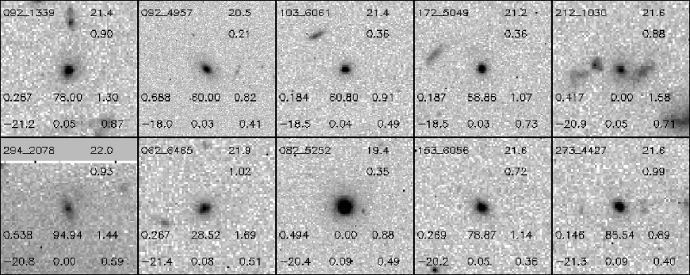
Figure 2.— Postage stamp images of 10 BSCs ($I$-band). The first 6 images (from top left to right) are for “good” BSCs, and the remaining images are for “possible” BSCs. Parameters listed in Fig. 2 are, from left to right, and from top to bottom, (1) ID# in our GSS catalog, (2) $I_{tot}$ magnitude, (3) redshift, (4) effective radius $r_{e}$(arcsec), (5) velocity dispersion $\sigma$, (6) observed $(V-I)$, (7) $B$-band absolute magnitude, (8) residual parameter $R$, (9) $B/T$. Boxes are scaled to be 50 kpc on its side.

Figure 3.— Redshift vs. $I$ magnitude of GSS galaxies. QS-E/S0s are marked with squares, “good” BSCs are marked with thick triangles, and “possible” BSCs are marked with thin triangles. The remaining galaxies are plotted as dots. Lines indicate trajectories of galaxies with two different absolute magnitudes at $z=0$: $M_{B}(z=0)=-19.37+5$ log$(h)$ ($\sim L^{*}$; Marzke et al. 1998) and $M_{B}(z=0)=-17.5+5$ log$(h)$. The solid lines assume passive luminosity evolution equal to $-1.7\times z$ in $B$-magnitudes (Im et al. 2001; Gebhardt et al. 2001; Koo et al. 2001), while dashed lines do not take the evolutionary correction into account. For the $K$-correction of the non-evolving models, we use the 13 Gyr-old SED of a model stellar population with 0.1 Gyr burst SFR, $z_{for}=11$, and the Salpeter IMF (GISSEL96).

Figure 4.— The OII [3727] doublet for representative BSCs. Most spectra here come from LRIS data. For 092_1339, we also show ESI data. The comparison between the LRIS and ESI data supports the accuracy of the line width measurements from lower-resolution LRIS data.

Figure 5.— $\sigma$ vs. $R_{hl,cir}$ for BSCs. The spaces occupied by typical local Hubble types are taken from Phillips et al. (1997). BSCs (triangles) are generally low-mass objects that lie in or near the space occupied by dEs). Red, QS-E/S0 galaxies with spectroscopic redshifts in Im et al. (2001) are plotted with squares showing a region where these QS-E/S0s with $I<22$ are expected to be found. The number plotted next to each point is the object number that appears in the first column of Table 1. The dotted lines show loci of constant mass from Eq. (1). Object #8 is not plotted as we have no $\sigma$ measured for it.

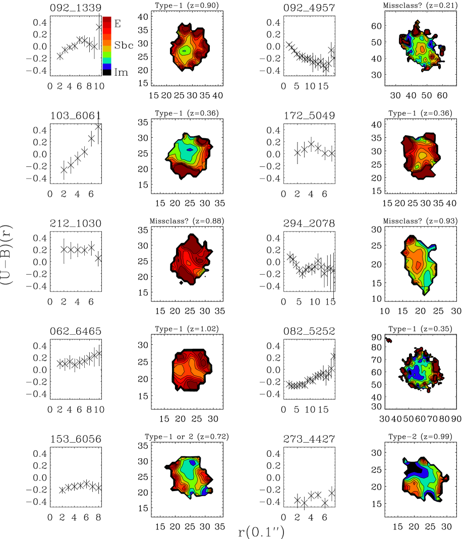
Figure 6.— Azimuthally averaged rest-frame $U-B$ color profiles plotted along their major axes, and 2-dimensional $U-B$ color maps of BSCs. For the 1-D color profile, the x-axis shows the distance from the center of the object, $r$, in 0.1 arcsec. For the 2-D color map, the x and y axes are also in units of pixels. Type-1 BSCs have a central region significantly bluer than the outer region, which in many cases is almost as red as typical field E/S0 galaxies. Note that the expected $U-B$ colors of passively evolving stellar populations after 0.1 Gyr bursts range from 0.1 to 0.5 depending on the age and metallicity at the redshift of interest (see text).

Figure 7.— Azimuthally averaged surface brightness profile of BSCs plotted along their major axis, as a function of distance from the center of the object. For each object, there are three panels, two for comparison with the $r^{1/4}$ bulge+ exponential disk profile, with distances indicated in units of $r^{0.25}$(0.1 arcsec) and $r$(0.1 arcsec), and a third for comparison with the double exponential profile, with distances given for $r$. A straight line is expected in the $r^{0.25}$ vs. SB plot for the $r^{0.25}$ law profile, while the same is true in the $r$ vs. SB plot for the exponential profile. The “X” marks show the measured SB. Models are drawn with the solid line (bulge+disk), the dashed line (bulge component), and dotted line (disk component), using outputs from the 2-dimensional GIM2D fit. Slight discrepancy between these data and the model exists; this is due to that (1) the aperture data are not deconvolved; (2) the aperture photometry is done with a fixed ellipticity while the bulge and disk components from the GIM2D fit have different ellipticities; and (3) faint neighbors affects the aperture photometry at the very outer regions.

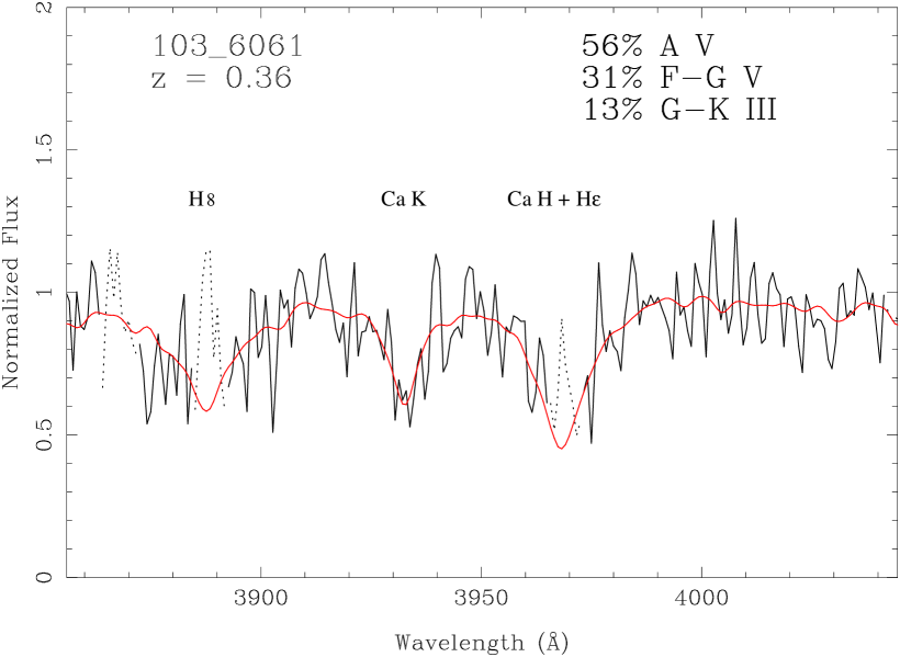
Figure 8.— The absorption-line spectrum of 103_6061 compared with the best-fit model spectrum. The spectrum is redshifted to the rest-frame and divided by the mean local continuum. The absorption-line velocity width ($\sigma_{abs}$) is measured using the maximum likelihood method as described in the text. We find $\sigma_{abs}<80$ km sec^-1. The best-fit mix of stellar types is indicated in the figure.

Figure 9.— Distribution of $\sigma_{FP}$ vs. $R_{hl,under}$ for the underlying red components of Type-1 BSCs. The spaces occupied by typical local Hubble types are taken from Phillips et al. (1997). Big diamonds indicate results based on a $r^{1/4}$ photo-bulge + exponential disk fit, while asterisks are for a double exponential fit. The line connecting diamonds and asterisks represents for each BSC how the position changes when the fitting method changes. The number plotted next to each point is the object number that appears in the first column of Table 1. The dotted lines show loci of constant mass from Eq. (1). Red, QS-E/S0 galaxies with spectroscopic redshifts in Im et al. (2001) are plotted with squares as in Fig. 5. Even using parameters of the underlying stellar population, BSCs appear to be low-mass objects.

Table 1Basic Data of Blue Spheroid Candidates

#	ID	RA	DEC	$z$	$I_{tot}$	$(V-I)$	$(U-B)_{rest}$	$M_{B}$	$B/T$	$R$	$\sigma_{em}$	$r_{hl,cir}$	$M_{vir}$	Type	Remarks
(1)	(2)	(3)	(4)	(5)	(6)	(7)	(8)	(9)	(10)	(11)	(12)	(13)	(14)	(15)
1	$092\_1339$	14:17:27.411	52:26:44.58	0.9031	21.40	1.30	-0.10	-21.22	0.87	0.05	$78$	2.2	1.9	1
					${}^{+0.03}_{-0.02}$	${}^{+0.04}_{-0.04}$	${}^{+0.02}_{-0.03}$	${}^{+0.03}_{-0.03}$	${}^{+0.06}_{-0.05}$		$\pm 6$	${}^{+0.4}_{-0.3}$
2	$092\_4957$	14:17:23.163	52:26:53.45	0.2105	20.52	0.81	-0.13	-18.03	0.41	0.03	$61$	5.6	3.7		Rot. curve with
					${}^{+0.03}_{-0.01}$	${}^{+0.03}_{-0.03}$	${}^{+0.03}_{-0.03}$	${}^{+0.03}_{-0.03}$	${}^{+0.02}_{-0.03}$		$\pm 30$	${}^{+0.1}_{-0.1}$			$V_{max}=130$km sec-1
3	$103\_6061$	14:17:27.242	52:26:08.37	0.3631	21.44	0.91	-0.15	-18.47	0.49	0.04	$61$	1.7	0.58	1
					${}^{+0.03}_{-0.02}$	${}^{+0.02}_{-0.04}$	${}^{+0.03}_{-0.03}$	${}^{+0.02}_{-0.02}$	${}^{+0.05}_{-0.06}$		$\pm 30$	${}^{+0.1}_{-0.1}$
4	$172\_5049$	14:16:31.410	52:17:26.24	0.3564	21.18	1.07	0.03	-18.51	0.73	0.03	$59$	1.7	0.54	1
					${}^{+0.03}_{-0.03}$	${}^{+0.04}_{-0.05}$	${}^{+0.05}_{-0.05}$	${}^{+0.03}_{-0.05}$	${}^{+0.04}_{-0.05}$		$\pm 30$	${}^{+0.1}_{-0.1}$
5	$212\_1030$	14:16:10.228	52:12:37.11	0.8778	21.63	1.58	0.06	-20.91	0.71	0.05	72?	3.8	2.8		Red early-type galaxy
					${}^{+0.06}_{-0.04}$	${}^{+0.06}_{-0.08}$	${}^{+0.04}_{-0.04}$	${}^{+0.06}_{-0.05}$	${}^{+0.14}_{-0.16}$		…	${}^{+0.8}_{-1.1}$			with a blue neighbor
6	$294\_2078$	14:15:23.216	52:01:41.56	0.9295	21.95	1.44	-0.01	-20.81	0.59	0.00	$95$	4.8	6.3		Rot. curve; late-type?
					${}^{+0.10}_{-0.06}$	${}^{+0.09}_{-0.13}$	${}^{+0.06}_{-0.07}$	${}^{+0.12}_{-0.07}$	${}^{+0.07}_{-0.14}$		$\pm 30$	${}^{+0.6}_{-0.6}$
7	$062\_6465$	14:17:41.030	52:30:26.60	1.0196	21.89	1.69	0.17	-21.35	0.51	0.08	$29$	2.4	0.29	1
					${}^{+0.05}_{-0.04}$	${}^{+0.06}_{-0.06}$	${}^{+0.03}_{-0.03}$	${}^{+0.06}_{-0.05}$	${}^{+0.07}_{-0.07}$		$\pm 30$	${}^{+0.2}_{-0.2}$
8	$082\_5252$	14:17:29.473	52:27:58.56	0.3480	19.38	0.88	-0.17	-20.44	0.49	0.09	…	4.9	…	1	$z$ from CFRS
					${}^{+0.01}_{-0.01}$	${}^{+0.01}_{-0.01}$	${}^{+0.01}_{-0.01}$	${}^{+0.01}_{-0.01}$	${}^{+0.01}_{-0.01}$			${}^{+0.1}_{-0.1}$
9	$153\_6056$	14:16:54.378	52:20:17.99	0.7206	21.63	1.14	-0.22	-20.19	0.36	0.05	$79$	2.2	1.8	1 or 2
					${}^{+0.03}_{-0.03}$	${}^{+0.05}_{-0.06}$	${}^{+0.04}_{-0.04}$	${}^{+0.03}_{-0.03}$	${}^{+0.03}_{-0.04}$		$\pm 30$	${}^{+0.1}_{-0.1}$
10	$273\_4427$	14:15:34.140	52:05:53.96	0.9890	21.56	0.89	-0.29	-21.32	0.40	0.09	$86$	1.1	1.1	2
					${}^{+0.03}_{-0.03}$	${}^{+0.03}_{-0.04}$	${}^{+0.02}_{-0.02}$	${}^{+0.04}_{-0.04}$	${}^{+0.03}_{-0.03}$		$\pm 30$	${}^{+0.1}_{-0.1}$

Note. — (1) Object number as used in Fig. 5; (2) Source ID given by FFC-XXYY, where FF is the subfield, C is the WFPC2 chip number, and XX and YY are the chip coordinates in units of 10 pixels; (3) Right Ascension (J2000); (4) Declination (J2000); (5) Spectroscopic redshift; (6) $I$-band total magnitude; (7) Observed $V-I$ color derived from the total model-fit magnitudes; (8) Rest-frame $U-B$ color, which is derived from $V-I$ and $z$ using the $K$-correction in Gebhardt et al. (2001); (9) Rest-frame $B$-band absolute magnitude; (10) Bulge to total light ratio measured in $I$ band; (11) Residual parameter measured in $I$ band; (12) Velocity dispersion $\sigma_{em}$ measured from emission lines in km sec^-1; (13) Circular aperture half-light radius in pixels. One pixel corresponds to 0.1 arcsec; (14) Dynamical mass in units of $10^{10}M_{\sun}$. These mass estimates are uncertain by a factor of 2; (15) BSC Type as described in the text; Errors associated with each quantity are $\pm 1\sigma$.

Table 2Structural Parameters of BSCs from Simultaneous $r^{1/4}$ + DISK Fit

#	ID	$B/T$	$r_{e,\rm maj}$	$r_{d,\rm maj}$	$(V-I)_{b}$	$(V-I)_{d}$	$(U-B)_{b,rest}$	$(U-B)_{d,rest}$	$e_{b}$	Inc	$\chi^{2}$
(1)	(2)	(3)	(4)	(5)	(6)	(7)	(8)	(9)	(10)	(11)	(12)
1	092_1339	0.85	3.4	0.6	1.63	0.45	0.10	-0.64	0.25	9	1.030
		${}^{+0.03}_{-0.04}$	${}^{+0.4}_{-0.2}$	${}^{+0.1}_{-0.1}$	${}^{+0.08}_{-0.07}$	${}^{+0.26}_{-0.30}$	${}^{+0.05}_{-0.04}$	${}^{+0.17}_{-0.20}$	${}^{+0.02}_{-0.02}$	${}^{+2}_{-6}$
2	092_4957	0.44	10.7	3.8	1.37	0.66	0.54	-0.30	0.36	53	1.010
		${}^{+0.02}_{-0.02}$	${}^{+0.2}_{-0.2}$	${}^{+0.1}_{-0.1}$	${}^{+0.13}_{-0.11}$	${}^{+0.06}_{-0.07}$	${}^{+0.16}_{-0.15}$	${}^{+0.06}_{-0.06}$	${}^{+0.05}_{-0.03}$	${}^{+1}_{-1}$
3	103_6061	0.50	3.1	0.8	1.29	0.60	0.26	-0.46	0.33	12	1.062
		${}^{+0.04}_{-0.04}$	${}^{+0.4}_{-0.3}$	${}^{+0.1}_{-0.1}$	${}^{+0.13}_{-0.14}$	${}^{+0.10}_{-0.12}$	${}^{+0.15}_{-0.15}$	${}^{+0.10}_{-0.11}$	${}^{+0.05}_{-0.15}$	${}^{+17}_{-8}$
4	172_5049	0.70	1.6	1.3	0.78	2.16	-0.28	1.39	0.27	17	1.024
		${}^{+0.03}_{-0.02}$	${}^{+0.1}_{-0.1}$	${}^{+0.1}_{-0.1}$	${}^{+0.05}_{-0.05}$	${}^{+0.26}_{-0.24}$	${}^{+0.05}_{-0.05}$	${}^{+0.37}_{-0.33}$	${}^{+0.02}_{-0.02}$	${}^{+11}_{-5}$
5	212_1030	0.52	1.6	5.4	1.79	1.59	0.19	0.08	0.02	5	1.051
		${}^{+0.04}_{-0.05}$	${}^{+0.2}_{-0.2}$	${}^{+0.3}_{-0.3}$	${}^{+0.20}_{-0.19}$	${}^{+0.20}_{-0.15}$	${}^{+0.12}_{-0.11}$	${}^{+0.12}_{-0.09}$	${}^{+0.02}_{-0.02}$	${}^{+5}_{-4}$
6	294_2078	0.46	4.1	3.6	3.11	0.76	0.85	-0.42	0.60	54	0.968
		${}^{+0.11}_{-0.10}$	${}^{+1.2}_{-1.0}$	${}^{+0.2}_{-0.2}$	${}^{+0.77}_{-0.63}$	${}^{+0.22}_{-0.25}$	${}^{+0.32}_{-0.29}$	${}^{+0.14}_{-0.16}$	${}^{+0.08}_{-0.08}$	${}^{+3}_{-4}$
7	062_6465	0.51	3.0	1.5	3.59	1.01	0.88	-0.20	0.10	42	1.008
		${}^{+0.07}_{-0.05}$	${}^{+0.5}_{-0.3}$	${}^{+0.1}_{-0.1}$	${}^{+1.40}_{-0.47}$	${}^{+0.12}_{-0.18}$	${}^{+0.17}_{-0.12}$	${}^{+0.07}_{-0.11}$	${}^{+0.04}_{-0.05}$	${}^{+2}_{-3}$
8	082_5252	0.47	10.6	2.1	1.17	0.67	0.14	-0.38	0.07	2	1.102
		${}^{+0.01}_{-0.01}$	${}^{+0.2}_{-0.2}$	${}^{+0.1}_{-0.1}$	${}^{+0.04}_{-0.05}$	${}^{+0.03}_{-0.04}$	${}^{+0.05}_{-0.05}$	${}^{+0.03}_{-0.03}$	${}^{+0.01}_{-0.02}$	${}^{+1}_{-1}$
9	153_6056	0.33	2.9	1.5	0.40	1.74	-0.76	0.24	0.44	50	1.042
		${}^{+0.04}_{-0.05}$	${}^{+0.2}_{-0.2}$	${}^{+0.1}_{-0.1}$	${}^{+0.16}_{-0.18}$	${}^{+0.15}_{-0.15}$	${}^{+0.12}_{-0.13}$	${}^{+0.12}_{-0.12}$	${}^{+0.13}_{-0.05}$	${}^{+2}_{-4}$
10	273_4427	0.39	3.3	0.7	1.01	0.79	-0.22	-0.36	0.41	74	1.083
		${}^{+0.04}_{-0.03}$	${}^{+0.7}_{-0.9}$	${}^{+0.1}_{-0.1}$	${}^{+0.19}_{-0.14}$	${}^{+0.09}_{-0.11}$	${}^{+0.11}_{-0.09}$	${}^{+0.06}_{-0.07}$	${}^{+0.08}_{-0.24}$	${}^{+1}_{-1}$

Note. — (1) Object number; (2) Object ID; (3) Bulge-to-total light ratio measured in the $I$-band from the simultaneous fit; (4) Major axis bulge effective radius in pixels. One pixel is equal to 0.1 arcsec; (5) Major axis disk scale length in pixels; (6) Observed $V-I$ color of bulge; (7) Observed $V-I$ color of disk; (8) Rest-frame $U-B$ color of bulge; (9) Rest-frame $U-B$ color of disk; (10) Ellipticity of the bulge component; (11) Disk inclination angle in degrees. For a face-on system, this value is equal to 0; (12) Reduced $\chi^{2}$ value of the 2-D fit.

Table 3Structural Parameters of BSCs from Simultaneous Double Exponential Fit

#	ID	$B/T$	$r_{d1,\rm maj}$	$r_{d2,\rm maj}$	$(V-I)_{d1}$	$(V-I)_{d2}$	$(U-B)_{d1,rest}$	$(U-B)_{d2,rest}$	$e_{d1}$	Inc	$\chi^{2}$
(1)	(2)	(3)	(4)	(5)	(6)	(7)	(8)	(9)	(10)	(11)	(12)
1	092_1339	0.52	2.9	0.6	1.57	1.09	0.06	-0.23	0.23	46	1.013
		${}^{+0.05}_{-0.04}$	${}^{+0.4}_{-0.4}$	${}^{+0.1}_{-0.1}$	${}^{+0.18}_{-0.17}$	${}^{+0.15}_{-0.15}$	${}^{+0.11}_{-0.10}$	${}^{+0.09}_{-0.09}$	${}^{+0.06}_{-0.06}$	${}^{+4}_{-7}$
2	092_4957	0.51	6.4	2.4	0.52	1.08	-0.43	0.17	0.41	51	1.003
		${}^{+0.04}_{-0.05}$	${}^{+0.1}_{-0.4}$	${}^{+0.1}_{-0.2}$	${}^{+0.12}_{-0.12}$	${}^{+0.15}_{-0.16}$	${}^{+0.12}_{-0.11}$	${}^{+0.19}_{-0.18}$	${}^{+0.03}_{-0.03}$	${}^{+2}_{-2}$
3	103_6061	0.71	0.8	2.7	0.75	1.29	-0.31	0.26	0.19	26	1.046
		${}^{+0.07}_{-0.10}$	${}^{+0.1}_{-0.1}$	${}^{+1.1}_{-0.5}$	${}^{+0.17}_{-0.16}$	${}^{+0.44}_{-0.53}$	${}^{+0.17}_{-0.16}$	${}^{+0.53}_{-0.56}$	${}^{+0.03}_{-0.05}$	${}^{+10}_{-16}$
4	172_5049	0.73	1.5	0.2	1.19	0.79	0.16	-0.26	0.21	30	1.033
		${}^{+0.02}_{-0.04}$	${}^{+0.1}_{-0.1}$	${}^{+0.1}_{-0.1}$	${}^{+0.08}_{-0.07}$	${}^{+0.17}_{-0.14}$	${}^{+0.09}_{-0.08}$	${}^{+0.17}_{-0.14}$	${}^{+0.03}_{-0.03}$	${}^{+6}_{-9}$
5	212_1030	0.78	2.6	0.1	1.84	1.74	0.22	0.16	0.18	80	1.054
		${}^{+0.02}_{-0.03}$	${}^{+0.3}_{-0.3}$	${}^{+0.2}_{-0.1}$	${}^{+0.16}_{-0.15}$	${}^{+0.26}_{-0.24}$	${}^{+0.10}_{-0.09}$	${}^{+0.16}_{-0.15}$	${}^{+0.08}_{-0.09}$	${}^{+4}_{-14}$
6	294_2078	0.55	2.2	5.2	1.97	0.61	0.30	-0.52	0.66	45	0.985
		${}^{+0.12}_{-0.15}$	${}^{+0.3}_{-0.4}$	${}^{+1.0}_{-1.2}$	${}^{+0.50}_{-0.36}$	${}^{+0.39}_{-0.32}$	${}^{+0.26}_{-0.20}$	${}^{+0.25}_{-0.21}$	${}^{+0.04}_{-0.07}$	${}^{+10}_{-17}$
7	062_6465	0.48	2.0	1.0	1.17	1.93	-0.11	0.29	0.19	49	1.016
		${}^{+0.21}_{-0.27}$	${}^{+0.7}_{-0.5}$	${}^{+0.1}_{-0.2}$	${}^{+0.66}_{-0.62}$	${}^{+0.80}_{-0.88}$	${}^{+0.35}_{-0.38}$	${}^{+0.34}_{-0.48}$	${}^{+0.08}_{-0.10}$	${}^{+11}_{-10}$
8	082_5252	0.34	6.4	1.8	0.81	0.80	-0.24	-0.25	0.14	1	1.101
		${}^{+0.02}_{-0.01}$	${}^{+0.1}_{-0.2}$	${}^{+0.1}_{-0.1}$	${}^{+0.06}_{-0.06}$	${}^{+0.03}_{-0.04}$	${}^{+0.06}_{-0.06}$	${}^{+0.04}_{-0.04}$	${}^{+0.02}_{-0.02}$	${}^{+3}_{-1}$
9	153_6056	0.48	0.9	2.6	1.00	1.44	-0.33	0.01	0.36	55	1.040
		${}^{+0.08}_{-0.21}$	${}^{+0.1}_{-0.3}$	${}^{+0.6}_{-0.6}$	${}^{+0.46}_{-0.50}$	${}^{+0.45}_{-0.68}$	${}^{+0.35}_{-0.37}$	${}^{+0.35}_{-0.51}$	${}^{+0.08}_{-0.07}$	${}^{+5}_{-9}$
10	273_4427	0.24	2.4	0.6	0.90	0.83	-0.29	-0.34	0.39	73	1.083
		${}^{+0.04}_{-0.05}$	${}^{+0.1}_{-0.2}$	${}^{+0.1}_{-0.1}$	${}^{+0.28}_{-0.24}$	${}^{+0.09}_{-0.09}$	${}^{+0.17}_{-0.15}$	${}^{+0.06}_{-0.05}$	${}^{+0.08}_{-0.10}$	${}^{+3}_{-2}$

Note. — (1) Object number; (2) Object ID; (3) Bulge-to-total light ratio measured in the $I$-band from the simultaneous fit; (4) Major axis exponential scale length for exponential photo-bulge in pixels. One pixel is equal to 0.1 arcsec; (5) Major axis disk scale length in pixels; (6) Observed $V-I$ color of exponential photo-bulge; (7) Observed $V-I$ color of photo-disk; (8) Rest-frame $U-B$ color of exponential photo-bulge; (9) Rest-frame $U-B$ color of photo-disk; (10) Ellipticity of the exponential photo-bulge component; (11) Disk inclination angle in degrees. For a face-on system, this value is equal to 0; (12) Reduced $\chi^{2}$ value of the 2-D fit.

Table 4Comparison between Velocity Dispersion Estimates

#	ID	$\sigma_{FP}$(km s-1)	$\frac{\sigma_{em}}{\sigma_{FP}}$
(1)	(2)	(3)	(4)
1	$092\_1339$	$136(92)\pm 10$	$0.57(0.85)\pm 0.06$
3	$103\_6061$	$42(21)\pm 4$	$1.44(2.87)\pm 0.73$
4	$172\_5049$	$111(61)\pm 8$	$0.53(0.96)\pm 0.27$
7	$062\_6465$	$97(88)\pm 14$	$0.29(0.33)\pm 0.31$
8	$082\_5252$	$72(50)\pm 3$	…
9	$153\_6056$	$67(74)\pm 7$	$1.18(1.06)\pm 0.46$
		$\langle\frac{\sigma_{em}}{\sigma_{FP}}\rangle$ $~{}~{}=$	$0.81(1.22)\pm 0.24$

Note. — (1) Object number; (2) Object ID; (3) Estimated $\sigma$ from fundamental plane relation for the underlying red component from the $r^{1/4}$ + disk fit and from the double exponential fit (numbers in parentheses); (4) Ratio of $\sigma$ from emission lines ($\sigma_{em}$) to $\sigma_{FP}$

References

- (1)
- (2) Abraham, R. G., Ellis, R. S., Fabian, A. C., Tanvir, N. R., & Glazebrook, K. 1999, MNRAS, 303, 641
- (3)
- (4) Anderdakis, Y. C., & Sanders, R. H. 1994, MNRAS, 267, 283
- (5)
- (6) Barton, E. J., Geller, M. J., & Kenyon, S. J. 2000, ApJ, 530, 660
- (7)
- (8) Babul, A., & Ferguson, H. C. 1996, ApJ, 458, 100
- (9)
- (10) Baugh, C. M., Cole, S., & Frenk, C. S. 1996, MNRAS, 283, 1361
- (11)
- (12) Bouwens, R., Broadhurst, T., & Silk, J. 1998, ApJ, 506, 557
- (13)
- (14) Brinchmann, J., et al. 1998, ApJ, 499, 112
- (15)
- (16) Bruzual A., G., & Charlot, S. 1993, ApJ, 405, 538
- (17)
- (18) Charlot, S., & Silk, J. 1994, ApJ, 432, 453
- (19)
- (20) de Jong, R. R. 1996, A&AS, 118, 557
- (21)
- (22) de Vaucouleurs 1948, Ann. d’Astrophys. 11, 247
- (23)
- (24) Driver, S. P., Couch, W. J., Phillipps, S., Windhorst, R. A. 1996 ApJ, 466, L5.
- (25)
- (26) Driver, S. P., et al. 1998, ApJ, 496, L93
- (27)
- (28) Faber, S. M., & Lin, D. N. C. 1983, ApJ, 266, L17
- (29)
- (30) Faber, S. M., et al. 1989, ApJS, 69, 763
- (31)
- (32) Franceschini, A., et al. 1998, ApJ, 506, 600
- (33)
- (34) Fomalont, E. B., Kellerman, K. I., Richards, E. A., Windhorst, R. A., & Partridge, B. P. 1997, ApJ, 475, L5
- (35)
- (36) Gallagher, J. S., & Wyse, R. F. G. 1994, PASP, 106, 1225
- (37)
- (38) Gebhardt, K., et al. 2001, ApJ, submitted
- (39)
- (40) Groth, E. J., et al. 1994, BAAS, 185, 5309
- (41)
- (42) Guzmán, R., et al. 1998, ApJ, 495, L13
- (43)
- (44) Guzmán, R., et al. 1997, ApJ, 489, 559
- (45)
- (46) Guzmán, R., et al. 1996, ApJ, 460, L5
- (47)
- (48) Hammer, F., Gruel, N., Thuan, T. X., Flores, H., & Infante, L. 2001, ApJ, in press
- (49)
- (50) Hernquist, L., & Quinn, P. J. 1987, ApJ, 312, 1
- (51)
- (52) Hornschemeier, A. E., et al. 2000, ApJ, 541, 49
- (53)
- (54) Illingworth, G. 1976, ApJ, 204, 73.
- (55)
- (56) Im, M., Casertano, S., Griffiths, R. E., Ratnatunga, K. U., & Tyson, J. A. 1995b, ApJ441, 494
- (57)
- (58) Im, M., Griffiths, R. E., Naim, A., Ratnatunga, K. U., Roche, N., Green, R. F., & Sarajedini, V. L., 1999 ApJ, 510, 82
- (59)
- (60) Im, M., Griffiths, R. E., Ratnatunga, K. U., Sarajedini, V. L. 1996, ApJ, 461, L79
- (61)
- (62) Im, M., Ratnatunga, K. U., Griffiths, R. E., & Casertano, S. 1995a, ApJ, 445, L15
- (63)
- (64) Im, M. et al. 2001, ApJ, in press
- (65)
- (66) Jansen, R. A., Fabricant, D., Franx, M., & Caldwell, N. 2000, ApJS, 126, 271
- (67)
- (68) Kauffmann, G., Charlot, S., & White, S. D. M. 1996, MNRAS, 283, L117
- (69)
- (70) Kent, S. M. 1985, ApJS, 59, 115
- (71)
- (72) Kobulnicky, H. A., & Gebhardt, K. 2000, AJ, 119, 1608
- (73)
- (74) Koo, D. C., Bershady, M. A., Wirth, G. D., Stanford, S. A., & Majewski, S. R. 1994, ApJ, 427, L9
- (75)
- (76) Koo, D. C., et al. 2001, in preparation
- (77)
- (78) Koo, D. C., et al. 1996, ApJ, 469, 535
- (79)
- (80) Lilly, S. J., et al. 1995, ApJ, 455, 75
- (81)
- (82) Lin, D. N. C., & Faber, S. M. 1983, ApJ, 266, L21
- (83)
- (84) Marleau, F. R., & Simard, L. 1998, ApJ, 507, 585
- (85)
- (86) Marzke, R., da Costa, L. N., Pellegrini, P. S., Willmer, C. N. A., & Geller, M. J. 1998, ApJ, 503, 617
- (87)
- (88) Menanteau, F., Abraham, R. G., & Ellis, R. S. 2000, MNRAS, in press
- (89)
- (90) Menanteau, F., et al. 1999, MNRAS, 309, 298
- (91)
- (92) Merritt, D. 1997, AJ, 114, 228
- (93)
- (94) Mihos, C. J., & Hernquist, L. 1994, ApJ, 437, L47
- (95)
- (96) Oke, J. B., et al. 1995, PASP, 107, 375
- (97)
- (98) Phillips, A. C., et al. 2001, in preparation
- (99)
- (100) Phillips, A. C., et al. 1997, ApJ, 489, 543
- (101)
- (102) Phillips, M. M., et al. 1986, AJ, 91, 1062
- (103)
- (104) Poveda, A. 1958, Bol. Obs. Tonantzintla y Tacubaya, No. 17.
- (105)
- (106) Ratnatunga, K., Griffiths, R. E., & Ostrander, E. J. 1999, AJ, 118, 86
- (107)
- (108) Rix, H.-W., Guhathakurta, P., Colles, M., & Ing, K. 1997, MNRAS285, 779
- (109)
- (110) Rhodes, J., Refregier, A., & Groth, E. J. 2000, ApJ, 536, 79
- (111)
- (112) Saha, P., & Williams, T. 1994, AJ, 107, 1295
- (113)
- (114) Schade, D., et al. 1999, ApJ, 525, 31
- (115)
- (116) Schade, D., et al. 1995, ApJ, 451, L1
- (117)
- (118) Scorza, C. et al. 1998, A&A, 131, 265
- (119)
- (120) Sheinis, A. I., Miller, J., Bolte, M., Sutin, B. 2000, in Proceedings of the SPIE, vol. 4008.
- (121)
- (122) Simard, L., et al. 2001, in preparation.
- (123)
- (124) Simard, L., et al. 1999, ApJ, 519, 563
- (125)
- (126) Telles, E. & Terlevich, R. 1993, Ap&SS, 205, 49
- (127)
- (128) Trager, S. C., Faber, S. M., Worthey, G., & Gonzalez, J. J. 2000, AJ, 119, 1645
- (129)
- (130) Vogt, N., et al. 2001a, in preparation
- (131)
- (132) Vogt, N., et al. 2001b, in preparation
- (133)
- (134) Young, P. J. 1976, ApJ, 81, 807.