SEARCH FOR SPATIAL VARIABILITY IN THE SOLAR ACOUSTIC SPECTRUM

Abstract

Motivated by the various examples of spatial variability in the power of the acoustic spectrum, we attempted to look for spatial variability in the peak frequency of the spectrum. However, the determination of this peak frequency on a spatial scale of a single pixel (8 arc seconds for the GONG data) is limited by the stochastic variations in the power spectrum presumably caused by the stochastic nature of the excitation process. Averaging over a large number of spectra (100 spectra from a 10 $\times$ 10 pixels area) produced stabler spectra. The peak frequencies of 130 such locations were found to be distributed with a FWHM of about 130 $\mu$Hz. A map of the spatial variation of this peak frequency did not show any strong feature with statistically significant deviation from the mean of the distribution. Likewise, the scatter in the peak frequencies masked the detection of magnetic field induced changes in the peak frequency. On a much larger scale, the N latitudes showed a slightly lower value of the peak frequency as compared to the S latitudes, although the difference (25 $\mu$Hz) is barely larger than the rms spread (20 $\mu$Hz).

guessConjecture

1 Introduction

The global oscillations of the Sun as measured by Dopplergrams produced in photospheric lines have maximum power around 5 min (Noyes, 1967, and references therein). The global nature of the oscillations was hitherto exploited by studying the ${\ell-\nu}$ diagnostic diagram, that used information obtained from each pixel on the solar disk in a collective manner (Deubener, 1972, and references therein). This technique has been extended in recent times to smaller pieces of the solar disk and to shorter timescales to produce local helioseismology using a variety of methods such as, Fourier-Hankel decomposition (Braun et al., 1987), ring diagrams (Hill, 1988), acoustic-imaging (Braun et al., 1992; Chang et al., 1997), time-distance seismology (Duvall et al., 1993), and helioseismic holography (Lindsey and Braun, 1998). Kumar et al. (2000) carried this exercise to the smallest possible resolution when they demonstrated that the shape and strength of the acoustic spectrum changed significantly in a sunspot relative to the quiet Sun. The variation in the shape of the spectrum can be quantified in terms of the variation in the peak frequency of the power spectrum. This parameter is relatively free of the effects of viewing angle and can therefore be readily adopted for studying the spatial variability of the acoustic spectrum. In this context, the spatial variability of the acoustic power over the solar surface is well documented, e.g., it has been seen that the absorption efficiency of p-mode power increases with the increasing magnetic field density (Braun, LaBonte and Duvall, 1990). The question is whether the peak frequency of the acoustic spectrum could be used as yet another parameter to map the spatial variability of the acoustic spectrum. In what follows, we attempt a preliminary investigation of this question using GONG data.

2 The data analysis

The data used here are from a time series of Dopplergrams for 11 and 12 May, 1997 for 560 minutes duration starting at 02:30 UT obtained by the GONG instrument at Udaipur Solar Observatory with a cadence of 1 minute. The Dopplergrams were derotated for mean solar rotation and registered with the first Dopplergram of each day. It is well known that the Dopplergrams, in addition to the p-modes, also exhibit variety of features, such as supergranulation pattern, meridional flows and solar rotation gradients. A two-point backward difference filter (GRASP/IRAF software package),

$$FilteredImage(t)=Image(t)-Image(t-1)$$ (1)

was applied to the Dopplergrams to enhance the p-mode oscillations above the other features. The temporal power spectrum was obtained for each pixel. This spectrum was smoothed by applying a digital filter, namely a Savitzky-Golay (S-G) filter (Press et al., 1992), to the power spectrum. This filter basically smooths the data by a window function of a predefined number of data points and a polynomial order with a proper weighting and then finds the maximum of the smoothed spectrum. We observe an optimal fit with a window of 32 data points and a polynomial of order 6. The peak frequency of the smoothed spectrum was then determined by selecting the discrete frequency in the appropriate frequency domain whose ordinate was greatest in the smoothed spectrum.

Figure 1: Sample spectrum for 4 individual pixels(thin solid lines). Shown in heavy solid lines are the fitted profiles estimated by S-G filter.

Figure 2: Power spectrum averaged over 10 $\times$ 10 pixels (thin solid line). Shown in heavy solid line is the fit estimated by S-G filter.

Figure 3: Power spectrum for a single pixel(thin solid line) for a time baseline of 4 hrs as compared to 560 minutes for the original data as shown in Figure 1. Shown in heavy solid line is the fit estimated by S-G filter.

Figure 4: Histograms of the distribution of the peak frequencies (for the 130 grids of the size 10 $\times$ 10 pixels) obtained for 11 May, 1997 (top panel) and 12 May, 1997 (bottom panel).

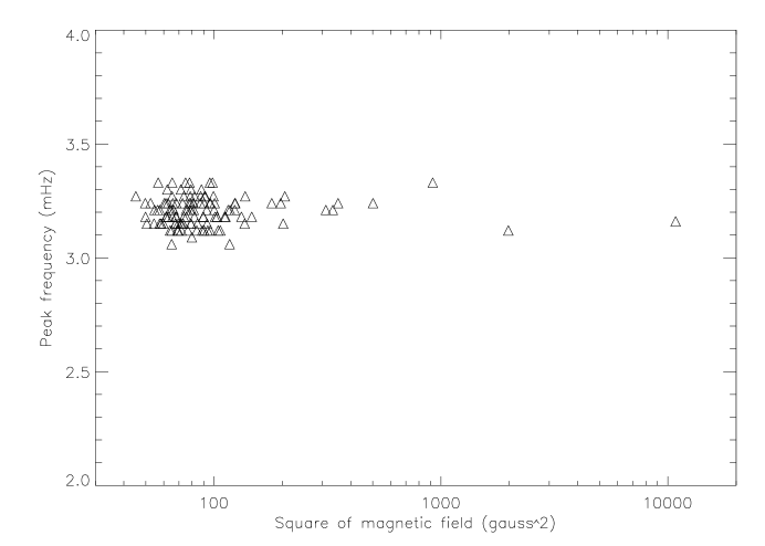
Figure 5: Scatter plot of the peak frequencies (for the 130 grids of the size 10 $\times$ 10 pixels) against $B^{2}$ (top panel) and ${|{\nabla B}|}$ (bottom panel) averaged over the 100 pixels for 12 May, 1997.

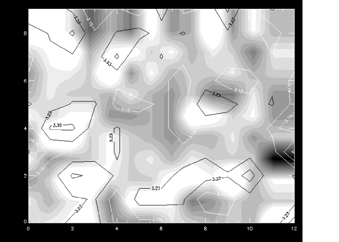
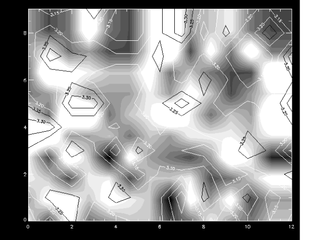
Figure 6: Map of the peak frequencies (for the 130 grids of the size 10 $\times$ 10 pixels) for 11 May, 1997 (top panel) and 12 May, 1997 (bottom panel). The contours are overlaid on a grey scale image of the 2-D function depicting the variation of the peak frequency with latitude and longitude. The abscissa denotes 50^∘ E to 50^∘ W and the ordinate 50^∘ S to 50^∘ N on the solar disk.

Figure 7: Cross-correlationgram of the maps of peak frequencies for 11 and 12 May, 1997.

Figure 8: Power spectrum averaged over 1300 pixels (thin solid line). Shown in thick solid line is the fit estimated by S-G filter.

3 Results

Figure 1 shows a sample spectrum for 4 individual pixels. It is seen that the peak of the spectrum appears at different frequency positions for the different spectra. We find that the rms variation of this peak frequency is fairly independent of the number of points chosen for the calculation of the rms value and is approximately 200 $\mu$Hz. At first sight, it would seem that the acoustic spectrum has a high spatial variability. However, the solar spectrum is most likely to be powered by a stochastic excitation process (Anderson, Duvall, and Jefferies, 1990). The power spectrum of such a stochastically excited oscillation would be highly variable, with peaks randomly appearing at various frequency positions due to the superposition of a large number of independent natural oscillations with random phases. If we assume that the power spectrum of each individual pixel is an independent realization of this random process, then the sum of several such spectra will produce more stable behaviour. We therefore summed 100 such spectra from a 10 $\times$ 10 pixels patch to obtain an average spectrum. In Figure 2, we have shown such an average power spectrum as well as the S-G fit applied to it for finding the peak frequency. It is seen that the uncertainty in the position of the peak ($\sim$ 70 $\mu$Hz), as determined by the S-G fit, does not improve with the averaging over 100 spectra. On the other hand, the uncertainty in fit almost doubles (146 $\mu$Hz) when we use a low resolution spectrum obtained from a 4 hrs sequence of the same data (Figure 3). Coming back to the 560 minutes time series, the aforesaid S-G algorithm is used to determine the peak of the spectrum for a raster of 130 grid points (each point providing an average spectrum for 10 $\times$ 10 pixels) spanning a rectangle of 10 latitudes (from 50^∘ S to 50^∘ N) by 13 longitudes (from 50^∘ E to 50^∘ W) on the Sun. It is to be noted that the size of the GONG Dopplergrams is different along the N-S and W-E directions because of the rectangular CCD pixels.

The histograms of the distribution of the peak frequencies obtained for 11 and 12 May, 1997 are shown in Figure 4. There is a FWHM spread of 124 $\mu$Hz and 170 $\mu$Hz for 11 and 12 May respectively. The scatter plots of these frequencies against $B^{2}$ and ${|{\nabla B}|}$ averaged over 10 $\times$ 10 pixels are shown in Figure 5. These plots show that the magnetic effects, if any, are smaller than the spread in the frequencies. Figure 6 shows the “map” of the peak frequencies on 11 and 12 May respectively. The cross-correlation of these two maps (Figure 7) shows no lag corresponding to solar rotation, ruling out the existence of any “feature” with lifetime greater than a day. The deviation in peak frequency as outlined by the contoured features in Figure 6 is not significantly greater than the half-width of the histograms (Figure 4). These “features” therefore do not merit more attention.

We now look for variation in the peak frequency on very large scales. In particular, we look for latitudinal variations. For this, we determine the average power spectrum of a band consisting of 10 pixels in latitude and 130 pixels in longitude. Figure 8 shows one such spectrum. A set of 81 such spectra were generated by box-car averages centred on a given latitude and spanning 10 pixels of latitude. We have thus 40 spectra in N latitudes and 40 in S latitudes with 1 at the equator. The mean of all the 40 peak frequencies at the N latitudes is 3.290 $\pm$0.020 mHz while the mean of all the S latitude peak frequencies is 3.315 $\pm$0.015 mHz. The difference in peak frequencies is 25 $\mu$Hz, which is barely greater than the rms spread. It remains to be seen whether data with better spectral resolution will be able to detect any N-S difference in the peak frequency.

4 Summary and Discussions

Motivated by the various examples of spatial variability in the power of the acoustic spectrum, we attempted to look for spatial variability in other parameters of the spectrum, which would be relatively less affected by the viewing angle. This concern about viewing angle, arises out of the need to look for latitudinal variation in the acoustic spectrum. The peak frequency in the acoustic spectrum seemed to be a good candidate. However, the precision of the determination of this peak frequency on a spatial scale of a single pixel (8 arc seconds for the GONG data) is limited by the stochastic variations in the power spectrum presumably caused by the stochastic nature of the excitation process. Averaging over a large number of spectra (100 spectra from a 10 pixel $\times$ 10 pixel area) produced more stable spectra. The peak frequencies of 130 such locations were found to be distributed with a FWHM of about 130 $\mu$Hz. A map of the spatial variation of this peak frequency did not show any strong feature with statistically significant deviation from the mean of the distribution. Likewise, the scatter in the peak frequencies masked the detection of magnetic field induced changes in the peak frequency. On a much larger scale, the N latitudes showed a slightly lower value of the peak frequency as compared to the S latitudes, although the difference (25 $\mu$Hz) is barely larger than the rms spread (20 $\mu$Hz).

The N-S difference in the peak frequency needs to be examined with data having higher spectral resolution. Similarly, the magnetic effects could be better discerned at higher spectral resolution, as was indicated in MDI data (Lindsey, 2001, personal communication). The present work has shown that the spectra of individual pixels can be treated as statistically independent realizations of the stochastically varying acoustic spectrum. In the same way, statistically independent realizations can be generated by using different initial times of the time series of a single pixel. Averaging over many such spectra can produce a stable spectrum for a single pixel. However, the detection of small scale spatial variability in the peak frequency obtained from such “temporally” averaged spectra of individual pixels would nevertheless require better spectral resolution. While the present work has shown the limits to which single station data can be pushed, a more significant “acoustic map” would perhaps be obtained from data having higher temporal resolution.

- [1] Anderson, E. R., Duvall, Jr., T. L., and Jefferies, S. M.: 1990, Astrophys. J. 364, 699.
- [2] Bhatnagar, A., Livingston, W. C., and Harvey, J. W.: 1972, Solar Phys. 27, 80.
- [3] Braun, D. C., Duvall, Jr., T. L., and LaBonte, B. J.: 1987, Astrophys. J. 319, L27.
- [4] Braun, D. C., LaBonte, B. J., and Duvall, Jr., T. L.: 1990, Astrophys. J. 354, 372.
- [5] Braun, D. C., Lindsey, C., Fan, Y., and Jefferies, S. M.: 1992, Astrophys. J. 392, 739.
- [6] Chang, H. -K. et al.: 1997, Nature 389, 825.
- [7] Deubener, F. -L.: 1972, Solar Phys. 22, 263.
- [8] Duvall Jr., T. L. et al.: 1993, Nature 362, 430.
- [9] Hill, F.: 1988, Astrophys. J. 333, 996.
- [10] Hindman, B. W., and Brown, T. M.: 1998, Astrophys. J. 504, 1029.
- [11] Kumar, B., Jain, R., Tripathy, S. C., Vats, H. O., and Deshpande, M. R.: 2000, Solar Phys. 191, 293.
- [12] Lindsey, C., and Braun, D. C.: 1998, Astrophys. J. 499, L99.
- [13] Lindsey, C.: 2001, Personal Communication
- [14] Noyes, R. W.: 1967, in R. N. Thomas (ed.), Proc. IAU Symp. 28 on Aerodynamic Phenomena in Stellar Atmospheres, New York: Academic Press, p. 293.
- [15] Nye, A. H., Cram, L. E., Thomas, J. H., and Beckers, J. M.: 1981, in Lawrence E. Cram and John H. Thomas (eds.), The Physics of Sunspots, Sac Peak Observatory Conference Proceedings, 14-17 July, 1981, p. 313.
- [16] Press, W. H., Teukolsky, S. A., Vellerling, W. T., and Flannery, B. P.: 1992, Numerical Recipies in FORTRAN, Cambridge University Press, Cambridge, p. 644.