Hard pomeron enhancement of ultrahigh-energy neutrino-nucleon cross-sections

Abstract

An unknown small-$x$ behavior of nucleon structure functions gives appreciable uncertainties to high-energy neutrino-nucleon cross-sections. We construct structure functions using at small $x$ Regge inspired description by A. Donnachie and P. V. Landshoff with soft and hard pomerons, and employing at larger $x$ the perturbative QCD expressions. The smooth interpolation between two regimes for each $Q^{2}$ is provided with the help of simple polynomial functions. To obtain low-$x$ neutrino-nucleon structure functions $F_{2}^{\nu N,\bar{\nu}N}(x,Q^{2})$ and singlet part of $F_{3}^{\nu N,\bar{\nu}N}(x,Q^{2})$ from Donnachie-Landshoff function $F_{2}^{ep}(x,Q^{2})$, we use the $Q^{2}$-dependent ratios $R_{2}(Q^{2})$ and $R_{3}(Q^{2})$ derived from perturbative QCD calculations. Non-singlet part of $F_{3}$ at low $x$, which is very small, is taken as power-law extrapolation of perturbative function at larger $x$. This procedure gives a full set of smooth neutrino-nucleon structure functions in the whole range of $x$ and $Q^{2}$ at interest.

Using these structure functions, we have calculated the neutrino-nucleon cross-sections and compared them with some other cross-sections known in literature. Our cross-sections turn out to be the highest among them at the highest energies, which is explained by contribution of the hard pomeron.

I Introduction

The interest to neutrino-nucleon cross-sections at very high energies, up $\sim 10^{21}$ eV, is stimulated by High Energy Neutrino Astronomy (HENA) (for a review see book ; GHS ). Ultra High Energy (UHE) neutrinos can be of accelerator and non-accelerator origin. In the former case UHE protons accelerated in astrophysical sources produce neutrinos in the chain of $\pi$- and $K$-decays, when UHE protons interact with ambient gas or with low energy photons. Since from observations we know that UHE protons exist with energies up to $3\times 10^{20}$ eV CR_3^10*20 , the maximum energy of neutrinos is expected up to $\sim 10^{19}$ eV. Astrophysical accelerators are usually connected with shock waves in SNe, AGNs, GRBs etc, but there could be also some other mechanisms of acceleration, such as acceleration in the strong electromagnetic wave and in strong electric field due to unipolar inductors (see Ref.book ).

Non-accelerator sources can provide neutrinos even with higher energies. These sources include production by Topological Defects (first suggested in Ref.HiSch ), by decays of superheavy dark matter particles and by annihilation of superheavy particles. Topological Defects in many cases become unstable and decompose to constituent fields, superheavy gauge bosons and Higgs particles, which then decay to hadrons and neutrinos. There could be the examples when the constituent superheavy fields are produced at annihilation (e.g. annihilation of monopole-antimonopole connected by string). Annihilation of dark matter particles (e.g. neutralino in Earth and Sun) gives another source of high energy neutrino production. The maximum energy of neutrinos from above-mentioned sources can reach the GUT scale.

High energy neutrino radiation from all sources is inevitably accompanied by other radiations, most notably by high energy gamma rays. Even in cases when high energy photons are absorbed in the source, their energy is partly transformed into low energy photon radiation: $X$-rays and thermal radiation. For sources transparent for high energy gamma radiation the upper limit on diffuse neutrino flux is imposed by the cascade electromagnetic radiation (see Ref.book ). Colliding with microwave photons, high energy photons and electrons give rise to electromagnetic cascades with most of energy being in the observed $100$ MeV – $10$ GeV energy range. The energy density of this cascade radiation should not exceed, according to EGRET observations, $\omega_{cas}\sim(1-2)\times 10^{-6}$ eV/cm³. Introducing the neutrino energy density for neutrinos with individual energies higher than $E$, $\omega_{\nu}(>E)$, it is easy to derive the following chain of inequalities (from left to right):

$$\omega_{cas}>\omega_{\nu}(>E)=\frac{4\pi}{c}\int_{E}^{\infty}EI_{\nu}(E)dE=\frac{4\pi}{c}EI_{\nu}(>E).$$ (1)

An upper bound on integral neutrino flux immediately follows from Eq. (1):

$$I_{\nu}(>E)<\frac{c}{4\pi}\frac{\omega_{cas}}{E}.$$ (2)

The latter inequality gives a powerful limit on the possible diffuse neutrino flux.

UHE neutrinos can be detected at the Earth due to their interactions with nucleons in CC and NC reactions,

$$\nu_{l}(\bar{\nu_{l}})+N(e^{-}) \rightarrow l^{\mp}(e^{\mp})+X,\quad\quad (CC)$$ (3)

$$\nu_{l}(\bar{\nu_{l}})+N(e^{-}) \rightarrow\nu_{l}(\bar{\nu_{l}})+X,\quad\quad (NC)$$ (4)

where $l=e,\mu,\tau$. These processes also modify the observed neutrino spectrum; neutrinos are both absorbed in (3) and driven to lower energies in (4) on their way from a source to a detector BGZR .

Cross-sections of $\nu e$-scattering are very small as compared with $\nu N$-cross-sections. An important exclusion is the resonant $\bar{\nu}_{e}e^{-}$-scattering BGRes :

$$\bar{\nu}_{e}+e^{-}\rightarrow W^{-}\rightarrow q_{i}+\bar{q}_{j}\rightarrow\mbox{\emph{hadrons}}.$$ (5)

The resonance energy of neutrino is $E_{0}=m_{W}^{2}/2m_{e}\simeq 6.4\times 10^{15}$ eV; the hadrons are produced as a spike with energy $E_{h}=E_{0}$. The number of resonant events in the underground detector with the number of electrons $N_{e}$ is given by the simple formula BGRes :

$$\nu_{res}=2\pi N_{e}\sigma_{eff}E_{0}I_{\bar{\nu}_{e}}(E_{0}),$$ (6)

where $\sigma_{eff}=(3\pi/\sqrt{2})G_{F}=3.0\times 10^{-32}$ cm² is the effective cross-section ($G_{F}$ is the Fermi constant) and $2\pi$ is the solid angle open for a deep underground detector (within another $2\pi$ angle neutrinos are absorbed).

A detailed discussion of all above mentioned processes can be found in Ref. Gandhi .

As regards $\nu N$-cross-sections, especially at extremely high energies, they are unknown yet. Really, to calculate the rate of high-energy events in a neutrino detector one actually needs the differential cross-sections of $\nu(\bar{\nu})N$ DIS in the whole range of kinematic variables $0\leq x\leq 1$ and $0\leq Q^{2}\leq\infty$. Such cross-sections, with QCD-effects being taken into account (see Ref. BGnucl ), may be expressed in terms of Parton Distribution Functions (PDF) in proton, in our case quarks, $q_{i}(x,Q^{2})$, where $q_{i}=u,d,c,s,t,b$. However, an influence of non-perturbative QCD-effects on nucleon Structure Functions (SF) at small both $Q^{2}$ and $x$ cannot be accurately estimated. It makes one to rely just on theoretical models, i.e. on various extrapolations.

In fact, differential neutrino-nucleon cross-section can be parameterized with the help of two structure functions, $F_{2}^{\nu N}(x,Q^{2})$ and $F_{3}^{\nu N,\bar{\nu}N}(x,Q^{2})$ (see e.g. Ref.’s deGroot ; FMR ; Hill ). In the case of CC scattering (3) these cross-sections are

$$\frac{d^{2}\sigma^{\nu N,\bar{\nu}N}_{CC}(E_{\nu},x,y)}{dxdy}=\frac{\sigma_{0}S_{W}}{2}\frac{(1-y+\frac{y^{2}}{2})F_{2}^{\nu N}(x,Q^{2})\pm(y-\frac{y^{2}}{2})xF_{3}^{\nu N,\bar{\nu}N}(x,Q^{2})}{(1+S_{W}xy)^{2}},$$ (7)

where $\sigma_{0}=\frac{G_{F}^{2}m_{W}^{2}}{\pi}$, $y=\frac{E_{h}}{E_{\nu}}$, $S_{W}=\frac{S}{m_{W}^{2}}$ and $S=2m_{N}E_{\nu}$, the $\pm$ sign corresponds to $\nu/\bar{\nu}$ cross-sections, respectively. It is useful to decompose the $F_{3}^{\nu N,\bar{\nu}N}$ into singlet and non-singlet parts,

$$F_{3}^{\nu N,\bar{\nu}N}(x,Q^{2})=F_{3}^{NS}(x,Q^{2})\pm F_{3}^{S}(x,Q^{2}).$$ (8)

The NC cross-sections (4) can be presented in a similar way, with $m_{W}$ replaced by $m_{Z}$, $S_{W}$ replaced by $S_{Z}=2m_{N}E_{\nu}/m_{Z}^{2}$, $\sigma_{0}=G_{F}^{2}m_{Z}^{2}/\pi$ and with structure functions given by

$$F_{2}^{\nu N(NC)}(x,Q^{2}) = (\delta_{1}^{2}+\delta_{2}^{2}+\delta_{3}^{2}+\delta_{4}^{2})F_{2}^{\nu N}+(\delta_{2}^{2}+\delta_{4}^{2}-\delta_{1}^{2}-\delta_{3}^{2})xF_{3}^{S},$$ (9)

$$F_{3}^{\nu N(NC)}(x,Q^{2}) = (\delta_{1}^{2}+\delta_{2}^{2}-\delta_{3}^{2}-\delta_{4}^{2})xF_{3}^{NS}.$$ (10)

The chiral couplings $\delta_{i}$ are

$$\delta_{1}=\frac{1}{2}-\frac{2}{3}\sin^{2}\theta_{W},\;\;\delta_{2}=-\frac{1}{2}+\frac{1}{3}\sin^{2}\theta_{W},\;\;\delta_{3}=-\frac{2}{3}\sin^{2}\theta_{W},\;\;\delta_{4}=\frac{1}{3}\sin^{2}\theta_{W};$$ (11)

we use $\sin^{2}\theta_{W}=0.23117$.

The quark contents of functions $F_{2}^{\nu N}$, $F_{3}^{NS}$ and $F_{3}^{NS}$ are as follows:

$$F_{2}^{\nu N}(x,Q^{2}) = x(q+\bar{q}),$$ (12)

$$F_{3}^{NS}(x,Q^{2}) = q-\bar{q},$$ (13)

$$F_{3}^{S}(x,Q^{2}) = 2(s-c+b-t),$$ (14)

with $q(x,Q^{2})=u+d+s+c+b+t$ and $\bar{q}(x,Q^{2})=\bar{u}+\bar{d}+\bar{s}+\bar{c}+\bar{b}+\bar{t}$.

Various parameterizations of $q_{i}(x,Q^{2})$, including recent versions of CTEQ, MRST, GRV, may be found in PDFLIB PDFLIB . All these parton distributions were obtained as LO/NLO solutions of Dokshitzer-Gribov-Lipatov-Atarelli-Parisi (DGLAP) equations with low $Q^{2}$ distributions $q_{i}(x,Q_{0}^{2})$ taken from experimental data at $Q_{0}^{2}\approx 1$ GeV². The calculated structure functions have been found valid in a wide range of $(x,Q^{2})$ parameter space:

$$10^{-5}\leq x\leq 1,\;\;\;1\mbox{{ GeV}}^{2}\leq Q^{2}\leq 10^{8}\mbox{{ GeV}}^{2}.$$

DGLAP approach is based on perturbative physics. The smallness of the QCD coupling constant $\alpha_{s}(k_{\perp}^{2})<1$ implies $k_{\perp}^{2}\geq Q_{0}^{2}$. The value of $Q_{0}\sim 0.3$ GeV determines the smallest allowed value of $k_{\perp}$ and can be viewed as mass of parton in QCD cascade. The minimal value of $x$ in perturbative approach is then determined $x_{min}\sim Q_{0}^{2}/S$, where $S=2m_{N}E_{\nu}$ for $\nu N$-scattering.

However, with $E_{\nu}$ increasing the ever smaller values of $x=\frac{Q^{2}}{Sy}$ get important in $\nu N$-scattering. It should be noted, that HENA actually promises the deepest insight in small-$x$ physics. Indeed, the record measurements today by HERA HERA relate to $F_{2}^{ep}(x,Q^{2})$ structure function with $x\lower 3.01385pt\hbox{$\;\stackrel{{\scriptstyle\textstyle>}}{{\sim}}\;$}10^{-5}$, while neutrino-nucleon SF with $E_{\nu}\sim 10^{19}$ eV are sensitive to $x\lower 3.01385pt\hbox{$\;\stackrel{{\scriptstyle\textstyle<}}{{\sim}}\;$}10^{-6}\div 10^{-8}$. As LO/NLO DGLAP dynamics evolves in $Q^{2}$-direction with $x$ being fixed, it provides no information about small-$x$ SF behavior. Moreover, the applicability of DGLAP approach to small-$x$ physics seems to be questionable. It was shown in Ref. Land that Mellin transform of DGLAP splitting matrix ${\mathbf{p}}(z)$, ${\mathbf{p}}(N)=\int_{0}^{1}dzz^{N}{\mathbf{p}}(z)$, suffers from singularities at $N=0$. These singularities arise in the perturbative expansion of $p_{qG}$ and $p_{GG}$ in powers of $\alpha_{S}$.

Nowadays, the only small-$x$ solution obtained in the framework of perturbative QCD is the BFKL-pomeron BFKL . However, the validity of this asymptotic solution is still to be checked. Though the importance of this approach is widely recognized, there were lately many criticisms of the pure BFKL-pomeron solution (see e.g. Ref. Dok and references therein).

A certain modification of BFKL-pomeron description has been proposed in Ref. KMS . It includes a unified BFKL/DGLAP evolution equation with a special ’consistency constraint’ imposed on BFKL component. Authors applied this approach to calculations of neutrino-nucleon cross-sections and checked manifestations of such solution in HENA.

In this paper we concentrate on the different approach to the small-$x$ physics, which is developing by A. Donnachie and P. V. Landshoff, hereafter DL, with coauthors Land . It is based on the Regge theory inspired description of small-$x$ $ep$-structure function, $F_{2}^{ep}(x,Q^{2})$. The authors have actually made the simplest possible assumption, namely, that contributions from branch points of the complex $l$-plane at $t=0$ are much weaker than those from poles. This hypothesis gives a rather good description of data and may be regarded as a guideline in $F_{2}^{ep}(x,Q^{2})$ small-$x$ extrapolation search. Though, predicting the power-law growth of cross-sections at high energies, this approach violates the unitarity.

According to DL, $F_{2}^{ep}(x,Q^{2})$ may be written down as a sum of three factorized terms,

$$F_{2}^{ep}(x,Q^{2})=\sum_{i=0}^{2}f_{i}(Q^{2})x^{-\epsilon_{i}},$$ (15)

where $\epsilon_{0},\epsilon_{1}$ and $\epsilon_{2}$ relate to the so-called ’hard pomeron’, ’soft pomeron’ and $\varrho,\omega,f,a$ exchanges, respectively. Shapes of $f_{i}(Q^{2})$ and values of $\epsilon_{i}$ are parameters; they are to be chosen so that to better fit the data. One of the best and the most convenient for our purposes set of $f_{i}(Q^{2})$, viz.

$$f_{0}(Q^{2}) = A_{0}\left(\frac{Q^{2}}{Q^{2}+a_{0}}\right)^{1+\epsilon_{0}}\left(1+X\ln\left(1+\frac{Q^{2}}{Q_{0}^{2}}\right)\right),$$ (16)

$$f_{1}(Q^{2}) = A_{1}\left(\frac{Q^{2}}{Q^{2}+a_{1}}\right)^{1+\epsilon_{1}}\frac{1}{1+\sqrt{Q^{2}/Q_{1}^{2}}},$$ (17)

$$f_{2}(Q^{2}) = A_{2}\left(\frac{Q^{2}}{Q^{2}+a_{2}}\right)^{1+\epsilon_{2}},$$ (18)

was proposed in Ref. Land . With

$$\begin{array}[]{lllllllll}\epsilon_{0}&=&0.418,&\epsilon_{1}&=&0.0808,&\epsilon_{2}&=&-0.4525,\\ A_{0}&=&0.0410,&A_{1}&=&0.387,&A_{2}&=&0.0504,\\ a_{0}&=&7.13,&a_{1}&=&0.684,&a_{2}&=&0.00291,\\ X&=&0.485,&Q^{2}_{0}&=&10.6,&Q^{2}_{1}&=&48.0,\end{array}$$ (19)

it describes $539$ data points with $\chi^{2}\approx 1.016$ per point.

It is worthy of note, that authors of this approach rather prefer fits with $f_{0}\propto Q^{\epsilon_{0}}$ at high $Q^{2}$ Land . In spite of slightly higher $\chi^{2}$, such fits are very attractive since their hard pomeron term looks similar to the perturbative BFKL solution. However, the direct identification of these two pomerons seems to remain dubious.

In the most recent version Land_New of their approach A. Donnachie and P. V. Landshoff propose a new parameterization of $F_{2}^{ep}(x,Q^{2})$ data. They have reduced the number of free parameters by including of the real photon cross-section data, $\sigma^{\gamma p}$. Authors argue that this new fit gives a good description of data also for $x>0.001$ and for $Q^{2}<5000$ GeV². With no additional parameters, they describe successfully the charm SF, $F_{2}^{c}(x,Q^{2})$, as well.

However, in the new fit authors use again the power-law dependence of coefficient $f_{0}(Q^{2})$ (16) at high $Q^{2}$. It works good at small $Q^{2}$, which are characteristic for photoproduction processes, but it does not extend to $Q^{2}\sim m_{W}^{2}$, which are typical for $\nu N$-scattering at $S>>m_{W}^{2}$. Such power-law behavior of the hard pomeron term cannot be reconciled with the quasi-logarithmic dependence on $Q^{2}$ of DGLAP SF at high $Q^{2}$. Therefore we cannot directly apply this new successful parameterization to the description of $\nu N$-cross-sections. Maybe it will be possible after a slight modification of the form of hard pomeron coefficient, which would coincide at small $Q^{2}$ with the original one. But in this paper we are to use the previous, logarithmic, parameterization (15)-(19).

In fact, all descriptions of small-$x$ SF are basically extrapolations with certain merits and demerits. In this paper we construct one more set of structure functions $F_{2}^{ep}$, $F_{2}^{\nu N}$, $F_{3}^{S}$ and $F_{3}^{NS}$. We want them

1. to be defined in the whole range of variables $0\leq x\leq 1$ and $0\leq Q^{2}\leq\infty$;

2. to comprise both perturbative at high-$x$ description, viz. CTEQ5 CTEQ , and non-perturbative at low-$x$ pure Regge theory approach of DL;

3. to be smooth over both variables with limited change of first derivative over $\log x$ in the interpolation zone.

Hereafter we call this approach DL+CTEQ5. We hope it is appropriate for the purposes of HENA.

Using DL+CTEQ5 functions, we calculate the $CC$, $NC$ and total ($CC+NC$) $\nu(\bar{\nu})N$-cross-sections and compare them with the results of Ref.’s Gandhi ; KMS . We also use for comparison the cross-sections obtained in the framework of trivial ’logarithmic’ extrapolation, hereafter Log+CTEQ5,

$$F_{i}^{\nu N,Log+CTEQ5}(x<x_{min},Q^{2})=F_{i}^{\nu N,CTEQ5}(x_{min},Q^{2})\left(\frac{x}{x_{min}}\right)^{\beta_{i}(Q^{2})},$$ (20)

$$\beta_{i}(Q^{2})=\left.\frac{\partial\ln F_{i}^{\nu N,CTEQ5}(x,Q^{2})}{\partial\ln x}\right|_{x=x_{min}};\;\;\;x_{min}=1\times 10^{-5},$$ (21)

which is analogous to the approach of Ref. BGZR . These SF smoothly shoot to the low-$x$ region from the CTEQ5 defined high-$x$ one. Starting values of functions and of their logarithmic derivatives over $x$ in such extrapolation are taken at the $x=x_{min}$ boundary of CTEQ5.

II Construction of DL+CTEQ5 structure functions

According to (7,9,10), neutrino-nucleon cross-sections depend just on $F_{2}^{\nu N}(x,Q^{2})$, $F_{3}^{S}(x,Q^{2})$ and $F_{3}^{NS}(x,Q^{2})$ SF, which quark contents is given by (12-14). However, the best small-$x$ data relate to $F_{2}^{ep}(x,Q^{2})$. Being just different combinations of quark density distributions, $q_{i}(x,Q^{2})$, these functions are bound indirectly. So, it is strongly desirable to make use of this information.

II.1 United $F_{2}^{ep}$ structure function

Let’s first obtain the united, smooth over $x$ and $Q^{2}$, structure function $F_{2}^{ep}(x,Q^{2})$, with small-$x$ behavior being in accordance with DL description (15-18) and with large-$x$ one being determined by CTEQ5. These functions are different, of course, so that we are to meet them smoothly.

First, to restrain the $Q^{2}$ divergency, we choose the DL parameter set (16-19). Really, at large $Q^{2}$ only the hard pomeron term (16) survives in (15), so that $F_{2}^{ep}(x,Q^{2})\propto\ln Q^{2}$. On the other hand, perturbative dynamics predicts an approximately logarithmic over $Q^{2}$ asymptotic growth of SF as well. In fact, the CTEQ5 $Q^{2}$-dependence of $F_{2}^{ep}$ at high $Q^{2}$ and $x\approx x_{\min}$ is close to logarithmic, but different; it rather looks like

$$F_{2}^{ep}(x,Q^{2})\propto(\ln Q^{2})^{1+\alpha(x)}$$ (22)

with $|\alpha(x)|\ll 1$. So, despite both functions fit to the same HERA data at $x=x_{\min}$, and therefore should coincide in a wide range of $Q^{2}$, they inevitably disperse at large $Q^{2}$. To reduce this discrepancy, we solved the equation $\alpha(x)=0$ numerically; the root is

$$x=x_{0}\simeq 2.527\times 10^{-5}.$$ (23)

We take the line $x(Q^{2})=x_{0}$ as one of boundaries of the interpolation zone. It is shown in the Fig. 1.

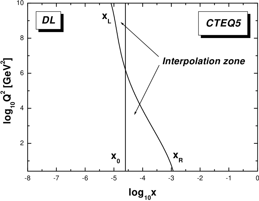
Figure 1: The borders of interpolation zone corresponding to $C=0.12$ (see (24)).

Luckily, $x_{0}$ is rather close to the left CTEQ5 boundary $x_{min}=1\times 10^{-5}$. At $x\simeq x_{0}$ both DL and CTEQ5 parameterizations still keep valid. It means that at relatively small $Q^{2}\lower 3.01385pt\hbox{$\;\stackrel{{\scriptstyle\textstyle<}}{{\sim}}\;$}500$ GeV² they are to be very close, if not equal. It is important, that at large $Q^{2}$ and $x=x_{0}$ both descriptions practically do not disperse.

On having reconciled the $Q^{2}$ behaviors, we take concern of smooth SF meeting over $x$ at each $Q^{2}$. The $x$-dependencies of these parameterizations are different. To meet them smoothly, we undertake an interpolation between $\ln F_{2}^{DL}$ and $\ln F_{2}^{CTEQ5}$ with the help of cubic over $\ln x$ polynomials; these procedure assures the first derivatives to be continuous in the whole interpolation zone.

So, keeping one border of the interpolation zone at $x(Q^{2})=x_{0}$ and varying the shape of another border, we call the latter $x_{L,R}(Q^{2})$, one gets a set of different interpolations. The subscripts $L,R$ mean that at small $Q^{2}$ we look for the right border, $x_{R}(Q^{2})$, while at large $Q^{2}$ we look for the left one, $x_{L}(Q^{2})$. The crossing takes place at $Q^{2}\approx 1.78\times 10^{6}$ GeV². These borders allow to extend the influence of DL description at small $Q^{2}$ to $x_{0}<x<x_{R}$, on the one hand, and, on the other hand, increase the influence range of the perturbative description at high $Q^{2}$ to smaller $x_{L}<x<x_{0}$. Such slant border seems us to be reasonable from the physical point of view.

The quality of interpolation may be parameterized by imposing of an additional condition:

$$\max\left|\left.\frac{\partial\ln F_{2}^{\nu N}(x,Q^{2})}{\partial\ln x}\right|_{x=x^{\prime}}-\left.\frac{\partial\ln F_{2}^{\nu N}(x,Q^{2})}{\partial\ln x}\right|_{x=x^{\prime\prime}}\right|<C,\quad\quad\forall\left\{x^{\prime},x^{\prime\prime}\in[x_{0},x_{L,R}]\right\}.$$ (24)

This actually constrains the maximum change of the tangent in the $x_{0},x_{L,R}$ range. The higher is $C$, the closer borders are allowed. However, at the same time the higher tangent change becomes possible in the interpolation zone. An optimum value of this parameter seems to be $C=0.12$.

The interpolation zone borders corresponding to this value of $C$ are plotted in the Fig. 1.

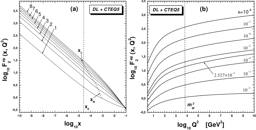
Figure 2: a) $F_{2}^{ep}(x,Q^{2})$ as a function of $x$ for different values of $\log_{10}Q^{2}=1,2,3,4,5,6,7,8$. Each label equals to the value of corresponding $\log_{10}Q^{2}$. The cubic spline interpolation over $x$ zone lies between two dash lines. b) $F_{2}^{ep}$ as the function of $Q^{2}$ for several values of $x$ denoted in the plot. The $m_{W}$ line corresponds to $Q^{2}=m_{W}^{2}$.

So, the described procedure results in $F_{2}^{ep}(x,Q^{2})$ with the desired properties. The $x$-dependence of these structure functions is plotted in Fig. 2a for several values of $Q^{2}$. In Fig. 2b the $Q^{2}$-dependence of the same functions is depicted for several values of $x$.

II.2 United neutrino-nucleon structure functions

Now let us turn to construction of neutrino-nucleon SF $F_{2}^{\nu N}(x,Q^{2})$, $F_{3}^{S}(x,Q^{2})$ and $F_{3}^{NS}(x,Q^{2})$. For relation of $F_{2}^{ep}(x,Q^{2})$ with $F_{2}^{\nu N}(x,Q^{2})$ a simple receipt has been proposed in Ref. FMR , hereafter FMR. Under an assumption that $i$-th flavor quark and anti-quark distributions in proton are equal, $q_{i}=\bar{q}_{i}$, and that $u=d=s=2c=2b$, the

$$F_{2}^{\nu N,FMR}(x,Q^{2})=\frac{72}{17}F_{2}^{ep}(x,Q^{2})$$

rule had been derived there. To get better description, we modify this approach by introducing of $Q^{2}$-dependent ratios $R_{2}(Q^{2})$ and $R_{3}(Q^{2})$. These ratio functions may be extracted from CTEQ5 at $x=x_{0}$ according to the rule

$$R_{2}(Q^{2}) = \frac{F_{2}^{\nu N,CTEQ5}(x_{0},Q^{2})}{F_{2}^{ep,CTEQ5}(x_{0},Q^{2})},$$ (25)

$$R_{3}(Q^{2}) = \frac{xF_{3}^{S,CTEQ5}(x_{0},Q^{2})}{F_{2}^{ep,CTEQ5}(x_{0},Q^{2})};$$ (26)

they are plotted in Fig. 3. These ratios differ from the constant values $R_{2}=\frac{72}{17}$ and $R_{3}=\frac{9}{17}$ (this value we derived using the assumption of Ref. FMR ), denoted in the picture as FMR. The difference is especially appreciable at small $Q^{2}$ due to the thresholds of heavy quarks production.

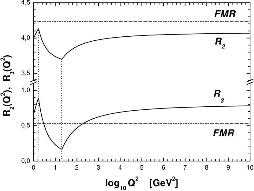
Figure 3: Ratios $R_{2}(Q^{2})=\frac{F_{2}^{\nu N}}{F_{2}^{ep}}$ and $R_{3}(Q^{2})=\frac{xF_{3}^{S}}{F_{2}^{ep}}$ calculated within CTEQ5 at $x=x_{0}$. The FMR lines correspond to analogous coefficients $R_{2}^{FMR}=\frac{72}{17}$ and $R_{3}^{FMR}=\frac{9}{17}$.

Combining ratios (25,26) with the constructed $F_{2}^{ep}(x,Q^{2})$ and assuming that these relations keep valid at lower values of $x$, we get the small-$x$

$$F_{2}^{\nu N}(x,Q^{2}) = R_{2}(Q^{2})\times F_{2}^{ep}(x,Q^{2}),$$ (27)

$$F_{3}^{S}(x,Q^{2}) = R_{3}(Q^{2})\times F_{2}^{ep}(x,Q^{2}).$$ (28)

At the next step we undertake the analogous to (24) cubic polynomial interpolation. It allows to smooth and restrict the $x$-discontinuity of these parameterizations.

To describe the negligible small-$x$ non-singlet structure function $F_{3}^{NC}(x,Q^{2})$, we use a trivial extrapolation of the corresponding CTEQ5 function in a way analogous to the Log+CTEQ5 (20,21). This completes the construction of united neutrino-nucleon SF.

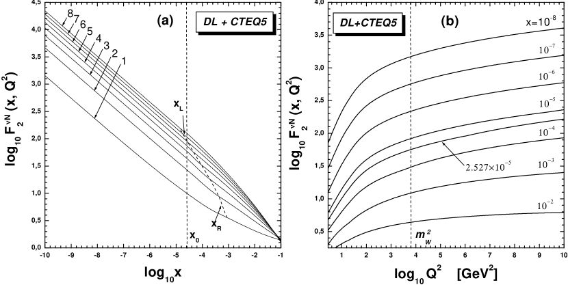
Figure 4: a) $F_{2}^{\nu N}(x,Q^{2})$ as a function of $x$ for different values of $\log_{10}Q^{2}=1,2,3,4,5,6,7,8$. Each label equals to the value of corresponding $\log_{10}Q^{2}$. The cubic spline interpolation over $x$ zone lies between two dash lines. b) $F_{2}^{\nu N}$ as the function of $Q^{2}$ for several values of $x$ denoted in the plot. The $m_{W}$ line corresponds to $Q^{2}=m_{W}^{2}$.

The characteristic features of the derived SF are illustrated in Fig.’s 4a and 4b. $F_{2}^{\nu N}(x,Q^{2})$ are depicted there for several values of $x$ versus $Q^{2}$ and for several values of $Q^{2}$ versus $x$.

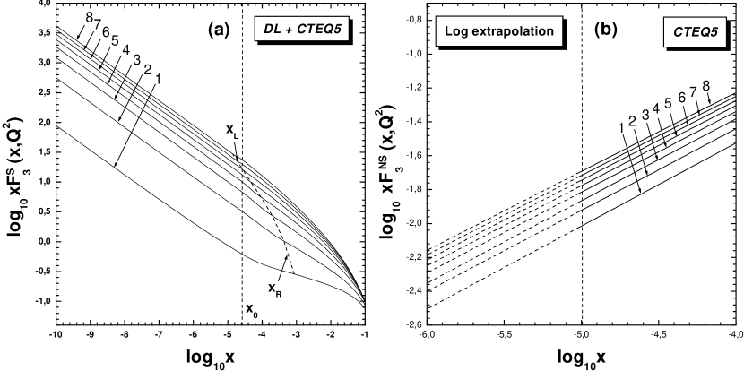
Figure 5: a) $xF_{3}^{S}(x,Q^{2})$ as a function of $x$ for different values of $\log_{10}Q^{2}=1,2,3,4,5,6,7,8$. Each label equals to the value of corresponding $\log_{10}Q^{2}$. The cubic spline interpolation over $x$ zone lies between two dash lines. b) The same plot as a) but for non-singlet $xF_{3}^{NS}(x,Q^{2})$. The dashed lines correspond to logarithmic extrapolation of corresponding perturbative function as described in the text.

The behavior of $xF_{3}^{S}(x,Q^{2})$ and of $xF_{3}^{NS}(x,Q^{2})$ as functions of $x$ are demonstrated in Fig.’s 5a and 5b.

III Comparison of cross-sections

Substituting the constructed DL+CTEQ5 SF into Eq.’s (7,9,10), we obtain the differential $\nu N$-cross-sections. The following integration over $x$ and $y$ and summation of CC- and NC-inputs gives the total cross-sections as functions of $E_{\nu}$.

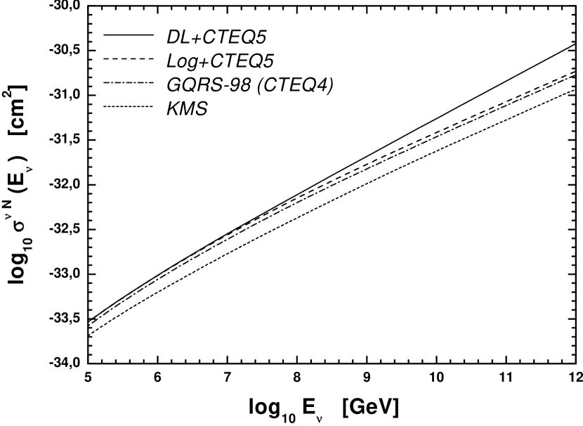
Figure 6: Total (CC+NC) DLGLAP+CTEQ5 $\nu N$-cross-sections. The analogous cross-sections of $Log+\emph{CTEQ5}$ extrapolation (20), of CTEQ4 parameterization by Gandhi et al. and of the united BFKL/DGLAP approach by Kwiecinski, Martin and Stasto, labelled as KMS are shown for comparison.

Denoted as DL+CTEQ5, this sum is shown in Fig. 6. For comparison we also plot here the corresponding cross-sections obtained in the framework of

a)

simple $Log+\emph{CTEQ5}$ extrapolation (20);

b)

CTEQ4 parameterization by Gandhi et al. Ref. Gandhi , denoted as GQRS-98 (CTEQ4);

c)

the united BFKL/DGLAP approach by Kwiecinski, Martin and Stasto KMS , labelled as KMS.

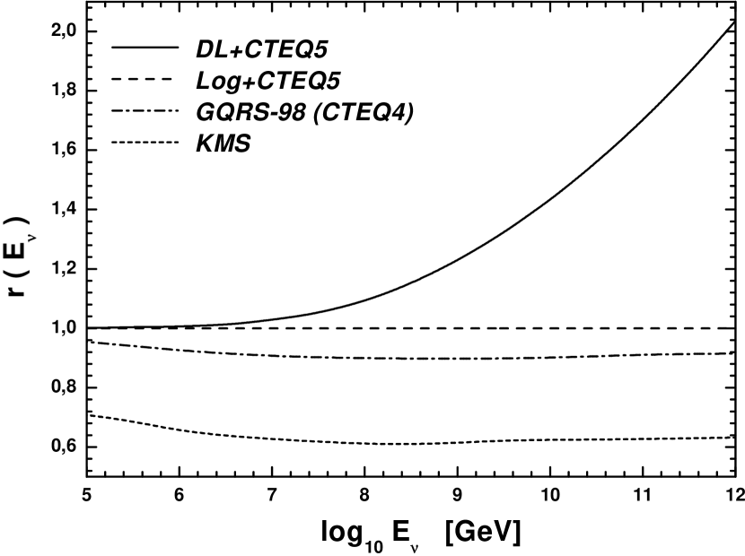
Figure 7: $r(E_{\nu})$ are ratios of the shown cross-sections and of Log+CTEQ5 cross-section.

Due to Regge hard pomeron pole, our approach predicts the more rapid growth of cross-sections at high energies. The differences between these calculations become especially clear in Fig. 7. We have divided each cross-section by corresponding cross-section of Log+CTEQ5. The ratios are plotted in the graph. At $E_{\nu}=1\times 10^{12}$ GeV the DL+CTEQ5 turns out to be twice as high as the logarithmic cross-section.

This difference is neither unexpected nor dramatic for HENA. One should remember that uncertainties in $\nu$-fluxes are much higher, while expected low measurement accuracy of future detectors and scarce statistics suggest, that such difference may be practically insignificant. However, we believe that rapid growth of $\nu N$-cross-sections may be eventually discovered in future giant detectors. This effect may play the essential role for UHE $\nu^{\,\prime}s$ predicted in the framework of TD models.

One should also keep in mind, that DL Regge theory approach violates unitarity. It implies that the predicted power-law growth of $\nu N$-cross-sections should be replaced at higher energies by, say, $\sigma\propto\ln^{2}E_{\nu}$ one. Though it is yet unknown where and how this occurs.

Conclusions

In this paper we have derived a new full set of smooth over $x$ and $Q^{2}$ $ep$- and $\nu N$-structure functions, which are defined for arbitrary allowable values of these kinematic variables. According to construction, these functions are in agreement with Regge theory inspired hard + soft pomeron small-$x$ parameterization by Donnachie and Landshoff, and coincide with perturbative $QCD$ parameterization by CTEQ5 at large $x$. For the smooth meeting of these structure functions over both $x$ and $Q^{2}$, the special interpolation zone boundaries have been defined.

We recalculate the known $F_{2}^{ep}(x,Q^{2})$ to $F_{2,3}^{\nu N}(x,Q^{2})$ structure functions at small $x$’s with the help of introduced ratios $R_{2,3}(Q^{2})$, which are derived from perturbative CTEQ5 description at $x_{0}=2.527\times 10^{-5}$.

Using these new structure functions, we have calculated the $\nu N$-cross-sections at extremely high energies and compared them with those earlier obtained a) within a simple logarithmic extrapolation of perturbative structure functions (Log+CTEQ5) and b) in papers Gandhi ; KMS . At small and moderate energies these cross-sections are practically indistinguishable. However, at extremely high energies non-perturbative hard pomeron dynamics causes a quicker rise of total $\nu N$-cross-sections with energy. Actually, these growth is the highest among all ever predicted in the framework of conventional theories.

We understand that pure pomeron behavior of SF cannot be a final answer since it violates unitarity. Nevertheless, we believe that such approach may be relevant in a wide range of energies involved in HENA.

References

- (1) V. S. Berezinsky, S. V. Bulanov, V. A. Dogiel, V. L. Ginzburg and V. S. Ptuskin, Astrophysics of Cosmic Rays, North-Holland (1990).
- (2) T. K. Gaisser, F. Halzen, and T. Stanev, Phys. Rep. 258, 174 (1995).
- (3) T. Abu-Zayyad et al., Proc. of 25th Int. Cosmic Ray Conf., Salt Lake City, Utah, eds. D. Kieda, M. Salamon and B. Dingus 3, 264 (1999); M. Takeda et al., Phys. Rev. Lett. 81, 1163 (1998).
- (4) Find reference or ask V.B.
- (5) V. S. Berezinsky, A. Z. Gazizov, G. T. Zatsepin and I. L. Rozental, Sov. J. Nucl. Phys. 43, 637 (1986).
- (6) V. S. Berezinsky and A. Z. Gazizov, JETP Lett. 25, 276 (1977); V. S. Berezinsky and A. Z. Gazizov, Sov. J. Nucl. Phys. 33, 230 (1981).
- (7) R. Gandhi, C. Quigg, M. H. Reno and I. Sarcevic, Phys. Rev. D 58, 093009 (1998).
- (8) Yu. M. Andreev, V. S. Berezinsky and A. Yu. Smirnov, Phys. Lett. B84, 247 (1979); V. S. Berezinsky and A. Z. Gazizov, Sov. J. Nucl. Phys. 29, 1589 (1979).
- (9) J. G. H. de Groot et al., Z. Phys. C – Part. Fields 1, 143 (1979).
- (10) G. M. Frichter, D. W. McKay and J. P. Ralston, Phys. Rev. Lett. 74, 1508 (1995).
- (11) G. C. Hill, Astropart. Phys. 6, 215 (1997).
-
(12)
One can find FORTRAN codes and many
references to the different PDF at web site
http://durpdg.dur.ac.uk/HEPDATA/PDF. - (13) H1: C. Adloff et al., Nucl. Phys. B497, 3 (1997); ZEUS: J. Breitweg et al., Phys. Lett. 407B, 432 (1997); H1: C. Adloff et al., Eur. Phys. J. C21, 33 (2001).
- (14) A. Donnachie and P. V. Landshoff, Phys. Lett. 437B, 408 (1998); P. V. Landshoff, hep-ph/9907392; R. D. Ball and P. V. Landshoff, J. Phys. G26, 672 (2000).
- (15) A. Donnachie and P. V. Landshoff, hep-ph/0105088.
- (16) E. A. Kuraev, L. N. Lipatov and V. S. Fadin, Sov. Phys. JETP 45, 199 (1977); Y. Y. Balitzkij and L. N. Lipatov, ibid. 28, 822 (1978); L. N. Lipatov, ibid. 63, 904 (1986).
- (17) Yu. L. Dokshitzer, hep-ph/9801372.
- (18) J. Kwiecinski, A. D. Martin and A. M. Stasto, Acta Phys. Polon. B31, 1273 (2000).
- (19) CTEQ collaboration - H. L. La et al., hep-ph/9903282; see also web site http://www.phys.psu.edu/∼cteq/