New Cosmological Data and the ‘Best-Fit’ FRW Universe

Abstract

Observational tests for the homogeneity of the Universe on large scales are reviewed. Assuming the Cosmological Principle we then estimate cosmological parameters by joint analysis of the Cosmic Microwave Background, Supernovae Ia, peculiar velocities, cluster abundance and redshift surveys. Our results are consistent with results obtained by other groups, suggesting a best-fit FRW Universe with ${\Omega_{\rm m}}=1-\lambda\approx 0.3$ and $H_{0}\approx 75$ km/sec/Mpc. We point out some potential problems with this currently popular model.

1 Introduction

The Cosmological Principle was first adopted when observational cosmology was in its infancy; it was then little more than a conjecture, embodying ’Occam’s razor’ for the simplest possible model. Observations could not then probe to significant redshifts, the ‘dark matter’ problem was not well-established and the Cosmic Microwave Background (CMB) and the X-Ray Background (XRB) were still unknown. If the Cosmological Principle turned out to be invalid then the consequences to our understanding of cosmology would be dramatic, for example the conventional way of interpreting the age of the Universe, its geometry and matter content would have to be revised. Therefore it is important to revisit this underlying assumption in the light of new galaxy surveys and measurements of the background radiations.

Like with any other idea about the physical world, we cannot prove a model, but only falsify it. Proving the homogeneity of the Universe is in particular difficult as we observe the Universe from one point in space, and we can only deduce isotropy directly. The practical methodology we adopt is to assume homogeneity and to assess the level of fluctuations relative to the mean, and hence to test for consistency with the underlying hypothesis. If the assumption of homogeneity turns out to be wrong, then there are numerous possibilities for inhomogeneous models, and each of them must be tested against the observations.

Here we examine the degree of smoothness with scale by considering redshift and peculiar velocities surveys, radio-sources, the XRB, the Ly-$\alpha$ forest, and the CMB. We discuss some inhomogeneous models and show that a fractal model on large scales is highly improbable. Assuming an FRW metric we evaluate the ‘best fit Universe’ by performing a joint analysis of cosmic probes.

2 Cosmological Principle(s)

Cosmological Principles were stated over different periods in human history based on philosophical and aesthetic considerations rather than on fundamental physical laws. Rudnicki (1995) summarized some of these principles in modern-day language:

$\bullet$ The Ancient Indian: The Universe is infinite in space and time and is infinitely heterogeneous.

$\bullet$ The Ancient Greek: Our Earth is the natural centre of the Universe.

$\bullet$ The Copernican CP: The Universe as observed from any planet looks much the same.

$\bullet$ The Generalized CP: The Universe is (roughly) homogeneous and isotropic.

$\bullet$ The Perfect CP: The Universe is (roughly) homogeneous in space and time, and is isotropic in space.

$\bullet$ The Anthropic Principle: A human being, as he/she is, can exist only in the Universe as it is.

We note that the Ancient Indian principle can be viewed as a ‘fractal model’. The Perfect CP led to the steady state model, which although more symmetric than the CP, was rejected on observational grounds. The Anthropic Principle is becoming popular again, e.g. in ‘explaining’ a non-zero cosmological constant. Our goal here is to quantify ‘roughly’ in the definition of the generalized CP, and to assess if one may assume safely the Friedmann-Robertson-Walker (FRW) metric of space-time.

3 Probes of Smoothness

3.1 The CMB

The CMB is the strongest evidence for homogeneity. Ehlers, Garen and Sachs (1968) showed that by combining the CMB isotropy with the Copernican principle one can deduce homogeneity. More formally the EGS theorem (based on Liouville theorem) states that “If the fundamental observers in a dust spacetime see an isotropic radiation field, then the spacetime is locally FRW”. The COBE measurements of temperature fluctuations $\Delta T/T=10^{-5}$ on scales of $10^{\circ}$ give via the Sachs Wolfe effect ($\Delta T/T=\frac{1}{3}\Delta\phi/c^{2}$) and Poisson equation rms density fluctuations of ${{\delta\rho}\over{\rho}}\sim 10^{-4}$ on $1000{\,h^{-1}\,{\rm Mpc}}$ (e.g. Wu, Lahav & Rees 1999; see Fig 3 here), i.e. the deviations from a smooth Universe are tiny.

3.2 Galaxy Redshift Surveys

Figure 1 shows the distribution of galaxies in the ORS and IRAS redshift surveys. It is apparent that the distribution is highly clumpy, with the Supergalactic Plane seen in full glory. However, deeper surveys such as LCRS and 2dFGRS (see below) show that the fluctuations decline as the length-scales increase. Peebles (1993) has shown that the angular correlation functions for the Lick and APM surveys scale with magnitude as expected in a universe which approaches homogeneity on large scales.

Figure 1: The distribution of galaxies projected on the sky in the IRAS and ORS samples. This is an Aitoff projection in Supergalactic coordinates, with $L=90^{\circ},B=0^{\circ}$ (close to the Virgo cluster) in the centre of the map. Galaxies within 2000 km/sec are shown as circled crosses; galaxies between 2000 and 4000 km/sec are indicated as crosses, and dots mark the positions of more distant objects. Here we include only catalogued galaxies, which is why the Zone of Avoidance is so prominent in these two figures. (Plot by M. Strauss, from Lahav et al. 2000).

Figure 2: The distribution of galaxies in part of the 2dFGRS, drawn from a total of 141,402 galaxies. The slices are 4 deg thick, towards the Northern Galactic Pole (left) and towards the Southern Galactic Pole (right). Not all 2dF fields within the slice have been observed at this stage; hence there are weak variations of the density of sampling. The image reveals a wealth of structure, including superclusters and voids, but the similarity between the two slices suggests that on large scales the universe is isotropic and homogeneous. (from Peacock et al. 2001).

Multifibre technology now allows us to measure redshifts of millions of galaxies. Two major surveys are underway. The US Sloan Digital Sky Survey (SDSS) will measure redshifts to about 1 million galaxies over a quarter of the sky. The Anglo-Australian 2 degree Field Galaxy Redshift Survey (2dFGRS) survey will measure redshifts for 250,000 galaxies selected from the APM catalogue. About 150,000 2dF redshifts have been measured so far (as of March 2001). The median redshift of both the SDSS and the 2dFGRS galaxy redshift surveys is ${\bar{z}}\sim 0.1$. While they can provide interesting estimates of the fluctuations on intermediate scales (e.g. Peacock et al. 2001; see Fig 2), the problems of biasing, evolution and $K$-correction, would limit the ability of SDSS and 2dF to ‘prove’ the Cosmological Principle. (cf. the analysis of the ESO slice by Scaramella et al 1998 and Joyce et al. 1999).

3.3 Peculiar Velocities

Peculiar velocities are powerful as they probe directly the mass distribution (e.g. Dekel et al. 1999). Unfortunately, as distance measurements increase with distance, the scales probed are smaller than the interesting scale of transition to homogeneity. Conflicting results on both the amplitude and coherence of the flow suggest that peculiar velocities cannot yet set strong constraints on the amplitude of fluctuations on scales of hundreds of Mpc’s. Perhaps the most promising method for the future is the kinematic Sunyaev-Zeldovich effect which allows one to measure the peculiar velocities of clusters out to high redshift.

The agreement between the CMB dipole and the dipole anisotropy of relatively nearby galaxies argues in favour of large scale homogeneity. The IRAS dipole (Strauss et al 1992, Webster et al 1998, Schmoldt et al 1999) shows an apparent convergence of the dipole, with misalignment angle of only $15^{\circ}$. Schmoldt et al. (1999) claim that 2/3 of the dipole arises from within a $40{\,h^{-1}\,{\rm Mpc}}$, but again it is difficult to ‘prove’ convergence from catalogues of finite depth.

3.4 Radio Sources

Radio sources in surveys have typical median redshift ${\bar{z}}\sim 1$, and hence are useful probes of clustering at high redshift. Unfortunately, it is difficult to obtain distance information from these surveys: the radio luminosity function is very broad, and it is difficult to measure optical redshifts of distant radio sources. Earlier studies claimed that the distribution of radio sources supports the ‘Cosmological Principle’. However, the wide range in intrinsic luminosities of radio sources would dilute any clustering when projected on the sky. Recent analyses of new deep radio surveys (e.g. FIRST) suggest that radio sources are actually clustered at least as strongly as local optical galaxies (e.g. Cress et al. 1996; Magliocchetti et al. 1998). Nevertheless, on the very large scales the distribution of radio sources seems nearly isotropic. Comparison of the measured quadrupole in a radio sample in the Green Bank and Parkes-MIT-NRAO 4.85 GHz surveys to the theoretically predicted ones (Baleisis et al. 1998) offers a crude estimate of the fluctuations on scales $\lambda\sim 600h^{-1}$ Mpc. The derived amplitudes are shown in Figure 3 for the two assumed Cold Dark Matter (CDM) models. Given the problems of catalogue matching and shot-noise, these points should be interpreted at best as ‘upper limits’, not as detections.

Figure 3: A compilation of density fluctuations on different scales from various observations: a galaxy survey, deep radio surveys, the X-ray Background and Cosmic Microwave Background experiments. The measurements are compared with two popular Cold Dark Matter models (with normalization $\sigma_{8}=1$ and shape parameters $\Gamma=0.2$ and $0.5$). The Figure shows mean-square density fluctuations $({{\delta\rho}\over\rho})^{2}\propto k^{3}P(k)$, where $k=1/\lambda$ is the wavenumber and $P(k)$ is the power-spectrum of fluctuations. The open squares at small scales are estimates from the APM galaxy catalogue (Baugh & Efstathiou 1994). The elongated ’boxes’ at large scales represent the COBE 4-yr (on the right) and Tenerife (on the left) CMB measurements (Gawiser & Silk 1998). The solid triangles and crosses represent amplitudes derived from the quadrupole of radio sources (Baleisis et al. 1998) and the quadrupole of the XRB (Lahav et al. 1997; Treyer et al. 1998). Each pair of estimates corresponds to assumed shape of the two CDM models. (A compilation from Wu, Lahav & Rees 1999).

3.5 The XRB

Although discovered in 1962, the origin of the X-ray Background (XRB) is still unknown, but is likely to be due to sources at high redshift (for review see Boldt 1987; Fabian & Barcons 1992). The XRB sources are probably located at redshift $z<5$, making them convenient tracers of the mass distribution on scales intermediate between those in the CMB as probed by COBE, and those probed by optical and IRAS redshift surveys (see Figure 3).

The interpretation of the results depends somewhat on the nature of the X-ray sources and their evolution. By comparing the predicted multipoles to those observed by HEAO1 (Lahav et al. 1997; Treyer et al. 1998; Scharf et al. 2000) we estimate the amplitude of fluctuations for an assumed shape of the density fluctuations (e.g. CDM models). Figure 3 shows the amplitude of fluctuations derived at the effective scale $\lambda\sim 600h^{-1}$ Mpc probed by the XRB. The observed fluctuations in the XRB are roughly as expected from interpolating between the local galaxy surveys and the COBE CMB experiment. The rms fluctuations ${{\delta\rho}\over{\rho}}$ on a scale of $\sim 600h^{-1}$Mpc are less than 0.2 %.

3.6 The Lyman-$\alpha$ Forest

The Lyman-$\alpha$ forest reflects the neutral hydrogen distribution and therefore is likely to be a more direct trace of the mass distribution than galaxies are. Unlike galaxy surveys which are limited to the low redshift Universe, the forest spans a large redshift interval, typically $1.8<z<4$, corresponding to comoving interval of $\sim 600{\,h^{-1}\,{\rm Mpc}}$. Also, observations of the forest are not contaminated by complex selection effects such as those inherent in galaxy surveys. It has been suggested qualitatively by Davis (1997) that the absence of big voids in the distribution of Lyman-$\alpha$ absorbers is inconsistent with the fractal model. Furthermore, all lines-of-sight towards quasars look statistically similar. Nusser & Lahav (2000) predicted the distribution of the flux in Lyman-$\alpha$ observations in a specific truncated fractal-like model. They found that indeed in this model there are too many voids compared with the observations and conventional (CDM-like) models for structure formation. This too supports the common view that on large scales the Universe is homogeneous. Another test for isotropy, based on the distribution of Supernovae Ia out to redshift $z\approx 1$ is described in Kolatt & Lahav (2001).

4 Is the Universe a Fractal ?

The question of whether the Universe is isotropic and homogeneous on large scales can also be phrased in terms of the fractal structure of the Universe. A fractal is a geometric shape that is not homogeneous, yet preserves the property that each part is a reduced-scale version of the whole. If the matter in the Universe were actually distributed like a pure fractal on all scales then the Cosmological Principle would be invalid, and the standard model in trouble. As shown in Figure 3 current data already strongly constrain any non-uniformities in the galaxy distribution (as well as the overall mass distribution) on scales $>300{\,h^{-1}\,{\rm Mpc}}$.

If we count, for each galaxy, the number of galaxies within a distance $R$ from it, and call the average number obtained $N(<R)$, then the distribution is said to be a fractal of correlation dimension $D_{2}$ if $N(<R)\propto R^{D_{2}}$. Of course $D_{2}$ may be 3, in which case the distribution is homogeneous rather than fractal. In the pure fractal model this power law holds for all scales of $R$.

The fractal proponents (Pietronero et al. 1997) have estimated $D_{2}\approx 2$ for all scales up to $\sim 500{\,h^{-1}\,{\rm Mpc}}$, whereas other groups have obtained scale-dependent values (for review see Wu et al. 1999 and references therein).

Estimates of $D_{2}$ from the CMB and the XRB are consistent with $D_{2}=3$ to within $10^{-4}$ on the very large scales (Peebles 1993; Wu et al. 1999). While we reject the pure fractal model in this review, the performance of CDM-like models of fluctuations on large scales have yet to be tested without assuming homogeneity a priori. On scales below, say, $30{\,h^{-1}\,{\rm Mpc}}$, the fractal nature of clustering implies that one has to exercise caution when using statistical methods which assume homogeneity (e.g. in deriving cosmological parameters). We emphasize that we only considered one ‘alternative’ here, which is the pure fractal model where $D_{2}$ is a constant on all scales.

5 More Realistic Inhomogeneous Models

As the Universe appears clumpy on small scales it is clear that assuming the Cosmological Principle and the FRW metric is only an approximation, and one has to average carefully the density in Newtonian Cosmology (Buchert & Ehlers 1997). Several models in which the matter in clumpy (e.g. ’Swiss cheese’ and voids) have been proposed (e.g. Zeldovich 1964; Krasinski 1997; Kantowski 1998; Dyer & Roeder 1973; Holz & Wald 1998; Célérier 1999; Tomita 1999). For example, if the line-of-sight to a distant object is ‘empty’ it results in a gravitational lensing de-magnification of the object. This modifies the FRW luminosity-distance relation, with a clumping factor as another free parameter. When applied to a sample of SNe Ia the density parameter of the Universe ${\Omega_{\rm m}}$ could be underestimated if FRW is used (Kantowski 1998; Perlmutter et al. 1999). Metcalf & Silk (1999) pointed out that this effect can be used as a test for the nature of the dark matter, i.e. to test if it is smooth or clumpy.

6 Cosmological Parameters from a Joint Analysis: a Cosmic Harmony ?

A simultaneous analysis of the constraints placed on cosmological parameters by different kinds of data is essential because each probe (e.g. CMB, SNe Ia, redshift surveys, cluster abundance and peculiar velocities) typically constrains a different combination of parameters. By performing joint likelihood analyses, one can overcome intrinsic degeneracies inherent in any single analysis and so estimate fundamental parameters much more accurately. The comparison of constraints can also provide a test for the validity of the assumed cosmological model or, alternatively, a revised evaluation of the systematic errors in one or all of the data sets. Recent papers that combine information from several data sets simultaneously include Webster et al. (1998); Lineweaver (1998); Gawiser & Silk (1998), Bridle et al. (1999, 2001), Eisenstein, Hu & Tegmark 1999; Efstathiou et al. 1999; and Bahcall et al. (1999).

While joint Likelihood analyses employing both CMB and LSS data are allowing more accurate estimates of cosmological parameters, they involve various subtle statistical issues:

• There is the uncertainty that a sample does not represent a typical patch of the FRW Universe to yield reliable global cosmological parameters.

• The choice of the model parameter space is somewhat arbitrary.

• One commonly solves for the probability for the data given a model (e.g. using a Likelihood function), while in the Bayesian framework this should be modified by the prior for the model and its parameters.

• If one is interested in a small set of parameters, should one marginalise over all the remaining parameters, rather than fix them at certain (somewhat ad-hoc) values ?

• The ‘topology’ of the Likelihood contours may not be simple. It is helpful when the Likelihood contours of different probes ‘cross’ each other to yield a global maximum (e.g. in the case of CMB and SNe), but in other cases they may yield distinct separate ‘mountains’, and the joint maximum Likelihood may lie in a ‘valley’.

• Different probes might be spatially correlated, i.e. not necessarily independent.

• What weight should one give to each data set ?

In a long term collaboration in Cambridge (Bridle et al. 1999, 2001; Efstathiou et al. 1999; Lahav et al. 2000) we have compared and combined in a self-consistent way the most powerful cosmic probes: CMB, galaxy redshift surveys, galaxy cluster number counts, type Ia Supernovae and galaxy peculiar velocities. These analyses illustrate the power of combining different data sets for constraining the fundamental parameters of the Universe. Our analysis suggests, in agreement with studies by other groups, that we live in a flat accelerating Universe, with comparable amounts of dark matter and ‘vacuum energy’ (cosmological constant). We have also addressed recently (Lahav et al. 2000; Lahav 2001) the issue of combining different data sets, which may suffer different systematic and random errors. We generalised the standard procedure of combining likelihood functions by allowing freedom in the relative weights of various probes. This is done by including in the joint likelihood function a set of ‘Hyper-Parameters’, which are dealt with using Bayesian considerations. The resulting algorithm, which assumes uniform priors on the logarithm of the Hyper-Parameters, is simple to implement. Here we show some examples of and results from the joint analysis. First combining two CMB data sets, and then combining CMB, Supernovae Ia and peculiar velocities.

7 Combining the CMB Boomerang and Maxima Data

The recent Boomerang (hereafter B; de Bernardis et al. 2000) and Maxima (hereafter M; Hanany et al. 2000) CMB anisotropy measurements yielded high-quality angular power spectra $C_{l}$ over the spherical harmonics $400\lower 2.15277pt\hbox{$\;\buildrel<\over{\sim}\;$}l\lower 2.15277pt\hbox{$\;\buildrel<\over{\sim}\;$}800$. An important factor in interpreting the data is the calibration error. The experimental papers quote calibration errors of 10% and 4% (1-sigma in $\Delta T/T$) for B and M, respectively. The measurements (with B data corrected upward by 10%, and M data corrected downward by 4 %) are shown in Figure 4, and they indicate a well defined first acoustic peak at $l\sim 200$, with less convincing second and third peaks at higher harmonics. These measurements favour (under certain assumptions) a flat universe, spectral index $n=1$ and baryon density ${\Omega_{\rm b}}h^{2}\sim 0.03$ (e.g. Jaffe et al. 2000), which is about 2-sigma higher than the Big-Bang Nucleosynthesis (BBN) value ${\Omega_{\rm b}}h^{2}\sim 0.0190\pm 0.0018$ (95 % CL; Burles et al. 2000). Note that the recent CBI result (Padin et al. 2000) gives a higher power (at $l\sim 600$) relative to B&M. Jaffe et al. (2000) fitted models after combining the B& M data sets into one set. We have taken a different approach for joint analysis of these two data sets by utilising the ‘Hyper-Parameters’ (Lahav 2001).

Figure 4: The Boomerang $\Delta T\over T$ data against spherical harmonic $l$ (top panel, calibrated by 1.10) and Maxima data (bottom panel, calibrated by 0.96). The line in each panel is for a $\Lambda$-CDM model with $n=1,{\Omega_{\rm m}}=1-\lambda=0.3,{\Omega_{\rm b}}h^{2}=0.03,{Q_{\rm rms}}=18\mu K$, and our ‘best fit’ $h=0.8$.

For simplicity, we restrict ourselves to a very limited set of cosmological models. We obtain theoretical CMB power-spectra using the CMBFAST and CAMB codes (Slejak & Zaldarriaga 1996; Lewis, Challinor & Lasenby 2000). We assume that CMB fluctuations arise from adiabatic initial conditions with Cold Dark Matter (CDM) and negligible tensor component, in a flat Universe with ${\Omega_{\rm m}}=0.3$, $\lambda\equiv\Lambda/(3H_{0}^{2})=1-{\Omega_{\rm m}}=0.7$, $n=1$, ${Q_{\rm rms}}=18\mu$K and ${\Omega_{\rm b}}h^{2}=0.03$. This choice is motivated by numerous other studies which combined CMB data with other cosmological probes (e.g. Jaffe et al. 2000, Bridle et al. 2000; Hu et al. 2000; see also the next section). We then investigate the constraints on the remaining parameter, the dimensionless Hubble constant, $h=H_{0}/$(100 km/sec/Mpc). Increasing $h$ decreases the height of the first acoustic peak, and makes few other significant changes to the angular power spectrum (e.g. Hu et al. 2000). The range in $h$ investigated here is ($0.5<h<1.1$).

The calibration of the data brings the two data sets to much better agreement. In fact, in this case the standard joint $\chi^{2}$ and the Hyper Parameters give the same result, $h=0.79$, with slightly smaller error bars in the HPs case ($\pm 0.04;95\%$ CL). We also tried the BBN value ${\Omega_{\rm b}}h^{2}=0.019$ which gives gives much poorer $\chi^{2}$ than the value ${\Omega_{\rm b}}h^{2}=0.03$ (e.g. Jaffe et al. 2000 and others).

The best fit Hubble constant is $H_{0}=79\pm 4$ km/sec/Mpc (95% CL, random errors only) for a fixed flat CDM ${\Omega_{\rm m}}=1-\lambda=0.3$ model with $n=1$, ${Q_{\rm rms}}=18\mu$K and ${\Omega_{\rm b}}h^{2}=0.03$. We note that if more cosmological parameters are left free and then marginalised over, the error in $h$ would typically be larger.

This combination of ${\Omega_{\rm m}}$ and $H_{0}$ corresponds gives for the age of the Universe 11.9 Gyr. Our derived $H_{0}$ is slightly higher but still consistent with the ‘final result’ of $H_{0}$ from Cepheids and other distance indicators (Freedman et al. 2000) $H_{0}=72\pm(3)_{r}\pm(7)_{s}$ km/sec/Mpc (1-sigma random and systematic errors).

8 Combining CMB, Supernovae Ia and Peculiar Velocities

A recent study (Bridle et al. 2001) is an example of combining 3 different data sets. We compared and combined likelihood functions for the matter density parameter ${\Omega_{\rm m}}$, the Hubble constant $h$, and the normalization $\sigma_{8}$ (in terms of the variance in the mass density field measured in an $8h^{-1}$ Mpc radius sphere) from peculiar velocities, CMB (including the Boomerang and Maxima data) and type Ia Supernovae. These three data sets directly probe the mass in the Universe, without the need to relate the galaxy distribution to the underlying mass via a “biasing” relation.

Our analysis assumes a flat $\Lambda$CDM cosmology with a scale-invariant adiabatic initial power spectrum and baryonic fraction as inferred from big-bang nucleosynthesis. We find that all three data sets agree well, overlapping significantly at the 2$\sigma$ level. This therefore justifies a joint analysis, in which we find a best fit model and $95\%$ confidence limits of ${\Omega_{\rm m}}=0.28\,(0.17,0.39)$, $h=0.74\,(0.64,0.86)$, and $\sigma_{8}=1.17\,(0.98,1.37)$. In terms of the natural parameter combinations for these data $\sigma_{8}{\Omega_{\rm m}}^{0.6}=0.54\,(0.40,0.73)$, ${\Omega_{\rm m}}h=0.21\,(0.16,0.27)$. Also for the best fit point, $Q_{\rm{rms-ps}}=19.7\mu$K and the age of the Universe is $13.0$ Gyr. Figure 5 illustrates these results.

This is quite in agreement from results form cluster abundance ${\Omega_{\rm m}}^{0.5}\sigma_{8}=0.5\pm 0.1$. (Eke et al. 1998). By combining the abundance of clusters with the CMB and IRAS Bridle et al. (1999) found ${\Omega_{\rm m}}=1-\lambda=0.36$, $h=0.54$, $\sigma_{8}=0.74$, and IRAS biasing parameter $b_{iras}=1.08$ (with error bars similar to those above).

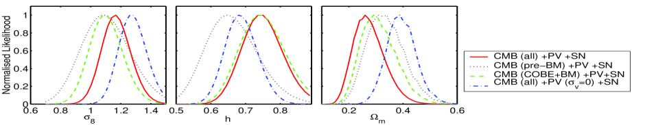
Figure 5: The 1-dimensional marginalised likelihood distributions from the joint PV, CMB and SN likelihood function. The main results are shown by the solid lines, which use the whole CMB data compilation, PV (marginalised over the field velocity dispersion $\sigma_{\rm v}$) and SN. The dotted lines show the likelihood functions when PV, SNe and just the pre-BM CMB data are used. The dashed line is the result when the CMB data is just COBE + BOOMERANG + MAXIMA-1. The result (using all the CMB data) when the uncorrelated velocity dispersion term is not included in the PV analysis ($\sigma_{\rm v}=0$) is shown by the dot-dashed line. (From Bridle etal. 2001.)

9 Discussion

Analysis of the CMB, the XRB, radio sources and the Lyman-$\alpha$ which probe scales of $\sim 100-1000{\,h^{-1}\,{\rm Mpc}}$ strongly support the Cosmological Principle of homogeneity and isotropy. They rule out a pure fractal model. However, there is a need for more realistic inhomogeneous models for the small scales. This is in particular important for understanding the validity of cosmological parameters obtained within the standard FRW cosmology.

Joint analyses of the CMB, IRAS, SNe, cluster abundance and peculiar velocities suggests ${\Omega_{\rm m}}=1-\lambda\approx 0.3$. The measurement of the Hubble constant from Cepheids and from the CMB suggests $H_{0}\approx 75$ km/sec/Mpc. While this is now a popular model there are potential problems with this set of parameters. There is no simple theoretical explanation why the present epoch contributions to matter ${\Omega_{\rm m}}$ and ’dark energy’ ($\lambda$) are nearly equal. Also, for the above model the age on the Universe is $\sim 13$ Gyr which is uncomfortably close to some estimates for the age of the Globular Clusters.

These issues will not doubt be revisited soon with larger and more accurate data sets. We will soon be able to map the fluctuations with scale and epoch, and to analyze jointly redshift surveys (2dF, SDSS) and CMB (MAP, Planck) data. These high quality data sets will allow us to study a wider range of models and parameters.

References

- [] Bahcall, N.A., Ostriker, J.P., Perlmutter, S. & Steinhardt, P.J., 1999, Science, 284, 148
- [] Baleisis, A., Lahav, O., Loan, A.J. & Wall, J.V. 1998, MNRAS, 297, 545
- [] Baugh C.M. & Efstathiou G. 1994, MNRAS , 267, 323
- [] de Bernardis, P. et al., 2000, Nature, 404, 955
- [] Boldt, E. A. 1987, Phys. Reports, 146, 215
- [] Bridle, S.L., Eke, V.R., Lahav, O., Lasenby, A.N., Hobson, M.P., Cole, S., Frenk, C.S., & Henry, J.P. 1999, MNRAS, 310, 565
- [] Bridle, S.L., Zehavi, I., Dekel, A., Lahav, O., Hobson, M.P. & Lasenby, A.N., 2001, MNRAS, 321, 333
- [] Buchert T & Ehlers, J. 1997, A&A, 320, 1
- [] Burles, S., Nollett, K.M. & Turner, M.S., 2000 (astro-ph/0008495)
- [] Célérier, M.N. 1999, submitted to A&A (astro-ph/9907206)
- [] Cress C.M., Helfand D.J., Becker R.H., Gregg. M.D. & White, R.L. 1996, ApJ, 473, 7
- [] Davis, M. 1997, Critical Dialogues in Cosmology, World Scientific, ed. N. Turok, pg. 13.
- [] Dekel, A. et al., 1999, ApJ, in press (astro-ph/9812197)
- [] Dyer, C.C. & Roeder, R.C. 1973, ApJ, 180, L31
- [] Ehlers, J., Geren, P & Sachs, R.K. 1968, J Math Phys, 9(9), 1344
- [] Efstathiou G., Bridle S. L., Lasenby A. N., Hobson M. P. & Ellis R. S. 1999, MNRAS, 303, L47
- [] Eisenstein, D.J., Hu, W. & Tegmark, M. 1999, ApJ, 518, 2
- [] Eke, V.R., Cole, S., Frenk, C.S. & Henry, J.P. 1998, MNRAS, 298, 1145
- [] Fabian, A. C. & Barcons, X. 1992, ARAA, 30, 429
- [] Freedman, W.L., et al., 2000, ApJ, in press (astro-ph/0012376)
- [] Gawiser, E. & Silk, J., 1998, Science, 280, 1405
- [] Hanany, S. et al., 2000, submitted to ApJL (astro-ph/0005123)
- [] Holz, D.E. & Wald, R.M. 1998, Phys Rev D, 58, 063501
- [] Hu, W., Fukugita, M., Zaldarriaga, M., Tegmark, M., 2000, submitted to ApJ (astro-ph/0006436)
- [] Jaffe et al., 2000, submitted to PRL (astro-ph/0007333)
- [] Joyce, M., Montuori, M., Sylos-Labini F. & Pietronero, L., 1999, A&A, 344, 387
- [] Kantowski, R. 1998, ApJ, 507, 483
- [] Kolatt, Ts. & Lahav, O., 2001, MNRAS, in press (astro-ph/0008041)
- [] Krasinski, A. 1997, Inhomogeneous Cosmological Models, Cambridge University Press, Cambridge
- [] Lahav O., Piran T. & Treyer M.A. 1997, MNRAS, 284, 499
- [] Lahav, O., Santiago, B.X., Webster, A.M., Strauss, M.A., Davis, M., Dressler, A. & Huchra, J.P. 2000, MNRAS, 312, 546
- [] Lahav, O., Bridle, S.L., Hobson, M.P., Lasenby, A.L., Sodré, L. 2000, MNRAS, 315, 45L
- [] Lahav, O., in the proceedings of IAU201 New Cosmological Data and the Values of the Fundamental Parameters Manchester 2001, Eds. A. Lasenby and A. Wilkinson, in press, (astro-ph/0012475)
- [] Lewis, A., Challinor, A. & Lasenby, A. 2000, ApJ, in press (astro-ph/9911177)
- [] Lineweaver, C. H. 1998, ApJ, 505, L69
- [] Magliocchetti, M., Maddox, S.J., Lahav, O.& Wall, J.V. 1998, MNRAS, 300, 257
- [] Metcalf, R. B. & Silk, J. 1999, ApJ L, 519, L1
- [] Nusser, A. & Lahav, O. 2000, MNRAS, 313, 39L
- [] Padin, S. et al, submitted to ApJ (astro-ph/0012211)
- [] Peebles, P. J. E. 1993, Principles of Physical Cosmology, Princeton University Press, Princeton.
- [] Peacock, J.A., et al., 2001, Nature, 410, 169
- [] Perlmutter et al. 1999, ApJ, 517, 565
- [] Pietronero, L., Montuori M., & Sylos-Labini, F. 1997, in Critical Dialogues in Cosmology, World Scientific, ed. N. Turok, pg. 24
- [] Rudnicki, K. 1995, The cosmological principles, Jagiellonian University, Krakow
- [] Scaramella, R. et al. 1998, A&A, 334, 404
- [] Scharf, C.A., Jahoda, K., Treyer, M., Lahav, O., Boldt, E. & Piran, T., , 2000, ApJ, 544, 49
- [] Schmoldt, I. et al. 1999, MNRAS, 304, 893
- [] Seljak, U. & Zaldarriaga, M. 1996, ApJ, 469, 437
- [] Strauss M.A. et al., 1992, ApJ, 397, 395
- [] Tomita, K. 1999 (astro-ph/9906027)
- [] Treyer, M., Scharf, C., Lahav, O., Jahoda, K., Boldt, E. & Piran, T. 1998, ApJ, 509, 531
- [] Webster, M.A., Lahav, O., & Fisher, K.B. 1998, MNRAS, 287, 425
- [] Webster, M., Bridle, S.L., Hobson, M.P., Lasenby, A.N., Lahav, O., & Rocha, G. 1998, ApJ, 509, L65
- [] Wu, K.K.S., Lahav, O. & Rees, M.J. 1998, Nature, 397, 225
- [] Zeldovich, Ya, B. 1964, Soviet Astron, 8, 13