The Imprint of Lithium Recombination on the
Microwave Background Anisotropies

Abstract

Following Loeb (2001), we explore the imprint of the resonant 6708Å  line opacity of neutral lithium on the temperature and polarization anisotropies of the cosmic microwave background (CMB) at observed wavelengths of $250$–$350\mu$m (0.9–1.2 THz). We show that if lithium recombines in the redshift range of $z=400$–$500$ as expected, then the standard CMB anisotropies would be significantly modified in this wavelength band. The modified polarization signal could be comparable to the expected polarization anisotropies of the far–infrared background on sub–degree angular scales ($\ell\gtrsim 100$). Detection of the predicted signal can be used to infer the primordial abundance of lithium, and to probe structure in the Universe at $z\sim 500$.

1 Introduction

The latest measurements of the anisotropies in the cosmic microwave background (CMB; see Halverson et al. 2001, Lee et al. 2001, Netterfield et al. 2001) imply that the days of “precision cosmology” have already arrived. Future ground and balloon based experiments, in combination with the satellite missions MAP in 2001 and Planck in 2007, will test current theoretical models to a sub–percent precision at photon wavelengths $\gtrsim 500\mu$m.

However, at far–infrared wavelengths of $\lesssim 350\mu$m, Loeb (2001) has recently shown that neutral lithium can strongly modify the CMB anisotropy maps, through absorption and re-emission at its resonant 6708Å transition from the ground state. Lithium is expected to recombine in the redshift interval $z\sim 400$–$500$ (Palla et al. 1995; Stancil et al. 1996, 1998). Despite the exceedingly low lithium abundance produced in the Big Bang, the resonant optical depth (Sobolev 1946) after lithium recombination is substantial,

$$\tau_{{}_{\rm LiI}}[\lambda(z)]=1.00f_{{}_{\rm LiI}}(z)\left({X_{{}_{\rm Li}}\over 3.8\times 10^{-10}}\right)\left({1+z\over 500}\right)^{3/2}.$$ (1)

for an observed wavelength of $\lambda(z)=[6708$Å$\times(1+z)]=335.4\mu{\rm m}\times[(1+z)/500]$. Here, $X_{{}_{\rm Li}}\approx 3.8\times 10^{-10}$ is the latest estimate of the lithium to hydrogen number density ratio (Burles et al. 2001), and $f_{{}_{\rm LiI}}(z)$ is the neutral fraction of lithium as a function of redshift (Palla et al. 1995; Stancil et al. 1996, 1998). Loeb (2001) argued that resonant scattering would suppress the original anisotropies by a factor of $\exp({-\tau_{{}_{\rm LiI}}})$, but will generate new anisotropies in the CMB temperature and polarization on sub–degree scales ($\ell\gtrsim 100$), primarily through the Doppler effect. Observations at different far–infrared wavelengths could then probe different thin slices of the early universe.

In this paper, we calculate in detail the effect of neutral lithium on both the polarization and temperature anisotropies of the CMB. §2 describes the modifications we have made to the standard code, CMBFAST (Seljak & Zaldarriaga 1996), in order to calculate these anisotropies. In §3, we describe our results and compare them to the foreground noise introduced by the far–infrared emission from galaxies and quasars. Finally, §4 summarizes the main conclusions of this work.

Throughout the paper we adopt the LCDM cosmological parameters of $\Omega_{0}\approx 0.25$, $\Omega_{\Lambda}=0.7$, $\Omega_{b}=0.05$, and $H_{0}\approx 70~{}{\rm km~{}s^{-1}~{}Mpc^{-1}}$, and units of $c=1$.

2 Method of Calculation

In order to compute the temperature and polarization fluctuations induced by lithium scattering, we complement the standard Thomson opacity ($\dot{\tau}_{{}_{T}}$) in CMBFAST by a new component ($\dot{\tau}_{{}_{\rm LiI}}$) which is assumed to have a narrow Gaussian shape in conformal time,

$$\dot{\tau} = \dot{\tau}_{{}_{\rm T}}(\eta)+\dot{\tau}_{{}_{\rm\ LiI}}(\eta,\nu)$$ (2)

$$= an_{e}\sigma_{T}+\tau_{{}_{\rm LiI}}{e^{-(\eta-\eta_{{}_{\rm LiI}})^{2}/2\sigma_{\eta}^{2}}\over\sqrt{2\pi\sigma_{\eta}^{2}}},$$

where, $\tau$ denotes optical depth, an overdot denotes a conformal time derivative, $a$ is the expansion factor, $\eta$ is conformal time ($a\ d\eta=dt$), $n_{e}$ is the number density of free electrons, and $\sigma_{T}$ is the Thomson cross–section. The lithium opacity depends both on time and observed photon frequency, $\nu$. We characterize this opacity by three parameters: the total optical depth $\tau_{{}_{\rm LiI}}$ given by equation (1), and the central time ($\eta_{{}_{\rm LiI}}$) and width ($\sigma_{\eta}$) of the Gaussian peak. The peak is set to a redshift $(1+z)=(\lambda/6708$ Å$)$ , where $\lambda=c/\nu$ is the observed wavelength. The actual (non-instrumental) width of the Gaussian is expected to be $[\Delta z/(1+z)]\sim 3\times 10^{-5}$ (Loeb 2001). Here we adopt $\sigma_{\eta}/\eta\sim 10^{-2}$, as dictated by a fiducial detector’s band–width.

The lithium opacity introduces a frequency dependence to the CMB anisotropies. Next we show that different frequencies couple only through the net drag force they provide on the baryons. Our discussion follows the notation of Ma & Bertschinger (1995).

We consider a density perturbation of comoving wave-vector ${\bf k}$. The photon distribution function can then be expanded to first order in the perturbation amplitude as,

$$f({\bf k},\hat{\bf n},\nu,\eta) = f_{0}(\nu)(1+\Psi({\bf k},\hat{\bf n},\nu,\eta)),$$

$$\Psi({\bf k},\hat{\bf n},\nu,\eta) = \sum_{l=0}^{\infty}(-i)^{l}(2l+1)\Psi_{l}(k,\nu,\eta)P_{l}(\hat{\bf k}\cdot\hat{\bf n}).$$ (3)

where $f_{0}(\nu)=2/h^{3}(e^{h\nu/kT_{0}}-1)$, and where $f$ is a function of perturbation wave-vector (${\bf k}$), time ($\eta$), and frequency ($\nu$) and propagation direction ($\hat{\bf n}$) of the photon. In the second line of equation (3), we have expanded the angular dependence of the distribution function in Legendre polynomials.

The distribution function $f({\bf k},\hat{\bf n},\nu,\eta)$ satisfies the Boltzmann equation. Since the Thomson cross–section is independent of frequency, the standard approach integrates the Boltzmann equation over photon frequencies and uses only one Boltzmann hierarchy to evolve the photon distribution function. In our case, the frequency dependence of the lithium cross–section implies that one should solve the hierarchy for different frequencies. Since the frequencies are coupled, one needs to follow all frequencies simultaneously, as done by Yu et al. (2001) for Rayleigh scattering. The coupling between different frequencies does not originate directly from the scattering term because lithium scattering does not change the photon frequency. As we show next, the coupling arises from the drag force on the baryons. Binary particle collisions allow the baryons to behave as a single fluid (Loeb 2001) which is subject to the sum of the forces applied by photons at all frequencies. In the limit of no drag force, the different frequencies decouple.

Next, we define the relative density contrast ($\delta_{\gamma}$) and velocity divergence of the photon fluid ($\theta_{\gamma}$) as,

$$\delta_{\gamma} = (a^{4}\bar{\rho}_{{}_{\rm CMB}})^{-1}{\int d^{3}\nu\ \nu f_{0}(\nu)\ \Psi_{0}(k,\nu,\eta)},$$

$$\delta\theta_{\gamma}(\nu) = (a^{4}\bar{\rho}_{{}_{\rm CMB}})^{-1}\ \ {3\over 4}k{\Psi_{1}(k,\nu,\eta)},$$

$$\theta_{\gamma} = \int d^{3}\nu\ \nu f_{0}(\nu)\ \delta\theta_{\gamma}(\nu).$$ (4)

With these definitions we can write the equation for the velocity divergence of the baryon fluid ($\theta_{b}=kv_{b}$),

$$\dot{\theta}_{b} = -{\dot{a}\over a}+c_{s}^{2}k^{2}\delta_{b}+{4\bar{\rho}_{{}_{\rm CMB}}\over 3\bar{\rho}_{b}}\left[\dot{\tau}_{\rm T}(\theta_{\gamma}-\theta_{b})+\int d^{3}\nu\ {\dot{\tau}}_{{}_{\rm\ LiI}}(\eta,\nu)\ \nu f_{0}(\nu)(\delta\theta_{\gamma}-\delta\theta_{b})\right]~{},$$

$$\delta\theta_{b} \equiv (a^{4}\bar{\rho}_{{}_{\rm CMB}})^{-1}\ {\theta_{b}},$$ (5)

where $c_{s}$ is the sound speed of the baryons, $\bar{\rho}_{{}_{\rm CMB}}$ and $\bar{\rho}_{b}$ are the mean energy densities of the CMB and the baryons, and $\delta_{b}$ is the baryon overdensity. The last term in the square brackets of equation (5) is responsible for the coupling between different photon frequencies. However, Figure 1 of Loeb (2001) implies that we may ignore the drag force on the baryons (due to either Thomson or lithium scattering) at the redshifts where the lithium opacity becomes important ($z\lesssim 500$). Consequently, we may solve the Boltzmann equation separately for each photon frequency by explicitly neglecting the transfer of momentum from the photons to the baryons due to lithium scattering. Even though momentum conservation is not strictly satisfied in this approach, the remaining correction is expected to be negligible.

The last change that we introduce to CMBFAST involves polarization. The cross–section for lithium scattering has a different dependence from Thomson scattering on both scattering angle and Stokes parameters. The scattering matrix for $(I_{\parallel},I_{\perp},U)$ (where the parallel and perpendicular directions are defined relative to the scattering plane) can be decomposed into two parts,

$${3\over 2}E_{1}\left(\begin{array}[]{ccc}\cos^{2}\Theta&0&0\\ 0&1&0\\ 0&0&\cos\Theta\\ \end{array}\right)+{1\over 2}E_{2}\left(\begin{array}[]{ccc}1&1&0\\ 1&1&0\\ 0&0&0\end{array}\right),$$ (6)

where $\Theta$ is the scattering angle. The first term is the usual Thomson (or Rayleigh) scattering matrix multiplied by a factor $E_{1}$, while the second term, which is proportional to $E_{2}$, does not generate polarization and is isotropic in angle. The two amplitudes depend on the quantum numbers of the resonant states, and satisfy $E_{1}+E_{2}=1$ (Chandrasekar 1960). For the transition between the ground state ($2S$) and first excited state ($2P$) of lithium, we get $E_{1}=1/3$ (Hamilton 1947; Chandrasekar 1960). Interference between the $2^{2}S$–$2^{2}P^{0}_{1/2}$ transition and the $2^{2}S$–$2^{2}P^{0}_{3/2}$ transition (Stenflo 1980) has a negligible effect on the polarization. This follows from the fact that $\tau_{{}_{\rm LiI}}\sim 1$; and for a given lithium atom, a photon will likely scatter when its frequency is separated from the line center by less than the natural width (37 MHz/$4\pi$), which is much smaller than the frequency separation between these transitions (10 GHz).

3 Results

The significance of the new opacity component can be assessed from the visibility function $\Upsilon(\eta)$. This function provides the probability distribution for the time of last scattering of the photons observed today at a conformal time $\eta_{0}$,

$$\Upsilon(\eta) = \dot{\tau}(\eta)e^{-\tau(\eta)},$$

$$\tau(\eta) = \int_{\eta}^{\eta_{0}}d\eta^{\prime}\dot{\tau}(\eta^{\prime}).$$ (7)

In Figure 1 we show the visibility functions for some of the models we consider later.

The observed anisotropies have two separate contributions, one from the standard last scattering surface at hydrogen recombination (decoupling), which is suppressed by $e^{-\tau_{{}_{\rm LiI}}}$, and a second new contribution that is generated by lithium scattering at lower redshifts. In the following sub-sections we will characterize this new contribution to the temperature and polarization anisotropies.

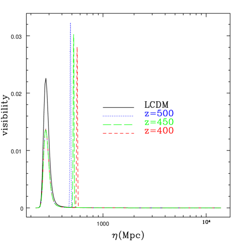
Figure 1: Visibility function for models with $\tau_{{}_{\rm LiI}}=0.5$ and LCDM. We show three examples, corresponding to resonant scattering at different redshifts, $z=400$, $z=450$ and $z=500$. The present–day value of the conformal time is $\eta_{0}=1.39\times 10^{4}$ Mpc.

3.1 Temperature and Polarization Anisotropies

Figures 2 and 4 show the predicted power spectra for the temperature and polarization anisotropies of the CMB at an observed wavelength of $\lambda=335.4\mu$m, corresponding to lithium scattering at $z=500$. The Stokes parameters are measured in $\mu K$. The figures compare the spectrum of fluctuations in standard LCDM (no lithium scattering) with two other models, each having a peak in $\dot{\tau}_{{}_{\rm LiI}}$ at a redshift of $z=500$, but with a total optical depth of either $\tau_{{}_{\rm LiI}}=0.5$ or $\tau_{{}_{\rm LiI}}=2.0$. Since at long wavelengths, $\lambda\gtrsim 500\mu$m, the LCDM fluctuations are not altered, precise mapping of these fluctuations by the MAP or Planck satellites will provide a reference power spectrum against which the lithium distortion can be measured.

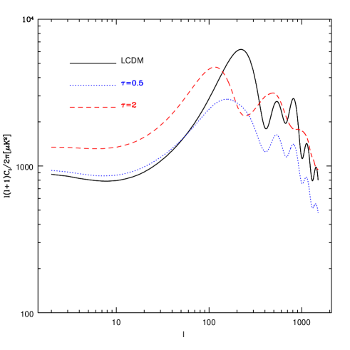
Figure 2: Temperature power spectra for the standard calculation (LCDM model), and two other models with lithium optical depths of $\tau_{{}_{\rm LiI}}=0.5$ or $\tau_{{}_{\rm LiI}}=2.0$ at $z=500$, for observations in a narrow–band around 335$\mu$m. The width of the $\dot{\tau}_{{}_{\rm LiI}}$ Gaussian in Eq. (2) is $\sigma_{\eta}/\eta=0.01$.

Figure 2 shows that for $\tau_{{}_{\rm LiI}}=0.5$ the small scale fluctuations are dominated by the suppressed anisotropies from recombination, resulting in a power spectrum which is similar in shape to that of the primary anisotropies but suppressed in amplitude. However, the $\tau_{{}_{\rm LiI}}=2$ case is very different. Here, the anisotropies are actually larger for many $l$’s than those expected without the lithium scattering, having a different functional dependence on $l$ than the standard case. The $e^{-\tau_{{}_{\rm LiI}}}$ suppression of the original anisotropies is sufficient to make them sub-dominant relative to the newly generated anisotropies at $z=500$.

There is an interesting difference between the primary anisotropies and those created by lithium scattering. In order to explain it, we introduce the integral solution for the temperature anisotropies,

$$\left({\Delta T\over T}+\psi\right)(k,\mu,\eta_{0})=\int_{0}^{\eta_{0}}d\eta\left[(\delta_{\gamma}/4+\psi+\mu v_{b})\Upsilon(\eta)+(\dot{\psi}+\dot{\phi})e^{-\tau(\eta)}\right]e^{ik\mu(\eta-\eta_{0})},$$ (8)

where $\mu$ is the cosine of the angle between the wave-vector and the direction of observation and $\phi$ and $\psi$ are the two gravitational potentials defined by the perturbed metric, $ds^{2}=a^{2}(\eta)[-(1+2\psi)d\eta^{2}+(1-2\phi)dx_{i}dx^{i}]$. While the contribution from recombination is dominated by the monopole term, ($\delta_{\gamma}/4+\psi$), the lithium anisotropies are dominated by the peculiar velocity term ($\propto v_{b}$) on most scales. We illustrate this in Figure 3 where we show the monopole and velocity contributions to the anisotropies in both the standard LCDM model and in a model that has a large optical depth $\tau_{{}_{\rm LiI}}=10$ at $z=500$. We chose such a large optical depth in order to suppress the original contribution from decoupling. The figure clearly shows that the anisotropies are dominated by the monopole term for the standard LCDM model for almost all values of $l$, while the opposite is true for the $\tau_{{}_{\rm LiI}}=10$ model. The new anisotropies are dominated by the monopole term only at very low multipoles, $l\lesssim 20$.

We can easily explain why the monopole no longer dominates for the lithium contribution. After recombination the monopole term decays by the free streaming of the photons while the velocity of the baryons continues to grow as they fall into the dark matter potential wells. For a perturbation mode of wave-vector $k$, the monopole term at conformal time $\eta$ after recombination, $\eta>\eta_{\rm rec}$, is approximately given by,

$$(\delta_{\gamma}/4+\psi)(\eta)=(\delta_{\gamma}/4+\psi)(\eta_{\rm rec})j_{0}\left[k(\eta-\eta_{\rm rec})\right],$$ (9)

where $j_{0}(x)$ is the spherical Bessel function. Equation (9) shows that the monopole term is small for $k(\eta-\eta_{\rm rec})\gg 1$ because of the decay in the Bessel function when its argument is large. Figure 1 shows that the new peak of the visibility function occurs at $\eta\sim 500\ {\rm Mpc}$ while $\eta_{\rm rec}\sim 300\ {\rm Mpc}$. We can translate the spatial wavenumber $k$ to angular scale using the conformal distance to the new peak in the visibility function, $d=(\eta_{0}-\eta)\approx\eta_{0}$. We find that $k(\eta-\eta_{\rm rec})\sim 1.6\times 10^{-2}l$, which explains why the monopole term is suppressed for $l\gg 60$.

While the monopole term decays between recombination and the lithium scattering surface, the velocity grows and thus produces anisotropies that are larger than those generated at decoupling in the $\tau_{{}_{\rm LiI}}=2$ case.

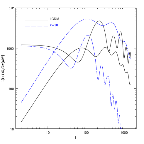
Figure 3: Velocity and temperature contribution to anisotropies for LCDM and for a model with $\tau_{{}_{\rm LiI}}=10$ at $z=500$. The curves that approach a finite value at low $l$ are the temperature contributions, and the curves that approach zero at low $l$ describe the velocity contributions.

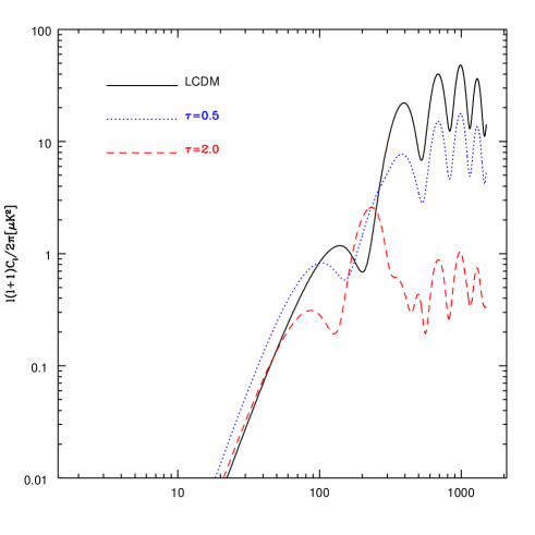
Figure 4: Polarization power spectra. Models are the same as in Fig. 2.

The physics of the polarization anisotropies is different from that of the temperature anisotropies. Since polarization is generated by the quadrupole moment, there are two competing effects that need to be considered. On the one hand, the quadrupole anisotropies are small at recombination, since they are suppressed relative to the velocity fluctuations by a factor $k\ \delta\eta$, where $\delta\eta$ is the width of the last scattering surface at recombination (Zaldarriaga & Harari 1995). In the new scenario the quadrupole is able to grow during the free streaming period between recombination and $z\sim 500$. This naturally leads to an increase in the polarization signal. The same effect increases the polarization anisotropies on large scales in models with a substantial optical depth to Thomson scattering after the universe reionizes (Zaldarriaga 1997). On the other hand, due to the nature of resonant–line scattering (Hamilton 1947; Chandrasekhar 1960), only $1/3$ of the cross–section generates polarization out of this quadrupole, while $2/3$ produces unpolarized radiation ($E_{1}=1/3,\ E_{2}=2/3$). Although the quadrupole is bigger at $z\sim 500$ than at recombination, the newly generated polarization is not as large. For example, Figure 4 shows that even for $\tau_{{}_{\rm LiI}}=2$, the polarization at high multipoles, $l\sim 1000$, is dominated by the suppressed signal from decoupling.

3.2 Cross–correlations and Difference Maps

Let us next consider two temperature anisotropy maps, obtained from observations at different wavelengths, $T^{a}(\hbox{\boldmath$\theta$})$ and $T^{b}(\hbox{\boldmath$\theta$})$. We define the following spectra in multipole space,

$$\langle T_{l}^{a}T_{l^{\prime}}^{a}\rangle = \delta_{ll^{\prime}}C_{l}^{aa},$$

$$\langle T_{l}^{b}T_{l^{\prime}}^{b}\rangle = \delta_{ll^{\prime}}C_{l}^{bb},$$

$$\langle T_{l}^{a}T_{l^{\prime}}^{b}\rangle = \delta_{ll^{\prime}}C_{l}^{ab},$$ (10)

with $\delta_{ll^{\prime}}$ being the Kronecker delta. Similar expressions can be written for $E$ and $B$–type polarization. We then define the cross–correlation coefficient,

$$CC_{l}={C_{l}^{ab}\over\sqrt{C_{l}^{aa}C_{l}^{bb}}}.$$ (11)

If $CC_{l}\rightarrow 1$ across a range of $l$’s, then the two maps are scaled versions of each other over that range.

Figures 5 and 6 show the correlation coefficients between maps of the anisotropies at different observed wavelengths, labelled by the redshift of the peak in the visibility function. They correspond to the correlation coefficient in three cases: (i) between the primary anisotropies and those measured at $\lambda=335.4\ \mu$m ($z=500$); (ii) between measurements at $\lambda=335.4\ \mu$m and $\lambda=301.8\ \mu$m ($z=450$); and (iii) between $\lambda=335.4\ \mu$m and $\lambda=268.3\ \mu$m ($z=400$).

The temperature correlation coefficient between the original map of the primary anisotropies and a map at 335.4 $\mu$m can be understood as follows. For low $l$, $CC_{l}\approx 1$ because the anisotropies are produced by long wavelength (small $k$) modes and the difference in conformal time between recombination and $z\sim 500$ (which we denote by $d_{\rm rec-500}$) is smaller than the perturbation wavelength , i.e. $(k\ d_{\rm rec-500}<<1)$. The fact that there are two different scattering surfaces does not make a difference for these modes.

On small scales, the situation is more complicated. The component of the anisotropies from decoupling, which is suppressed by a factor $e^{-\tau_{{}_{\rm LiI}}}$, drives the cross–correlation coefficient to unity, because its suppression results merely in rescaling. However, the newly generated anisotropies are uncorrelated with those coming from decoupling if they are produced by wavelengths that are smaller than $d_{\rm rec-500}$, i.e. if $k\ d_{\rm rec-500}\sim(d_{\rm rec-500}/d_{\rm rec})l\sim 1.6\times 10^{-2}l\gg 1$. The newly generated anisotropies tend to drive the cross–correlation coefficient to zero on small scales.

In Figure 5 we also show the cross–correlations between maps at observed wavelengths for which $\dot{\tau}_{{}_{\rm LiI}}$ peaks at $z=400$, $z=450$, and $z=500$. For a given angular scale, the anisotropies generated by the second peak of the visibility function are different only if the conformal distance between the two peaks is much larger than the wavelength of the perturbation producing the anisotropies on that scale. This explains why the departure from $CC_{l}=1$ occurs on smaller scales for the correlation between $z=500$ and $z=450$ than for that between $z=500$ and $z=400$. Also, if the anisotropies in the two maps have a substantial contribution from decoupling, then the correlation coefficient will not approach zero even on small scales where the newly generated anisotropies in the two maps are uncorrelated. The significance of this primary contribution from decoupling is suppressed when $\tau_{{}_{\rm LiI}}$ increases, as illustrated by the $\tau_{{}_{\rm LiI}}=0.5$ and $\tau_{{}_{\rm LiI}}=2.0$ panels of Figure 5.

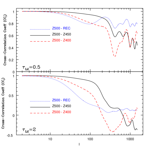
Figure 5: Correlation coefficients for temperature anisotropies at three different wavelengths corresponding to lithium resonances at $z=400$ (268$\mu$m), $z=450$ (302$\mu$m) and $z=500$ (335$\mu$m). The dotted lines show the correlation coefficient between the standard (long wavelength) anisotropies and those with lithium scattering at $z=500$; the solid line shows the correlation between the anisotropies for 302 $\mu$m and 335$\mu$m ($z=500$ and $z=450$); and the dashed lines correspond to 335$\mu$m and 268$\mu$m ($z=500$ and $z=400$). The upper panel shows the case of $\tau_{{}_{\rm LiI}}=0.5$ and the lower panel shows the case of $\tau_{{}_{\rm LiI}}=2.0$.

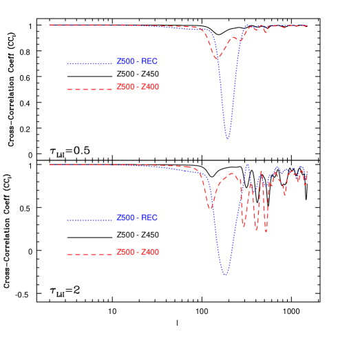
Figure 6: Correlation coefficient for polarization. The upper panel shows the case of $\tau_{{}_{\rm LiI}}=0.5$, and the lower panel shows the case of $\tau_{{}_{\rm LiI}}=2.0$

The correlation coefficient for polarization which is shown in Figure 6, can be explained along similar lines. On small scales, the polarization anisotropies are dominated by the suppressed contribution from recombination, and so $CC_{l}\rightarrow 1$. The dominance of the new anisotropies over the primary ones at $l\sim 200$, makes the correlation coefficient between primary and $z=500$ deviate away from unity around that scale. However, among neighboring frequencies the cross–correlation approaches unity near $l\sim 200$, because the distance between the peaks of the visibility function is not sufficient to decorrelate the contributions from the relevant $k$ modes.

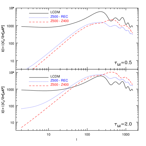
Figure 7: Difference power spectra for temperature anisotropies. In the upper panel $\tau_{{}_{\rm LiI}}=0.5$, and in the lower panel $\tau_{{}_{\rm LiI}}=2.0$.

In Figures 7 and 8 we show the difference power spectra for two maps at different observed wavelengths. We define $\delta T(\hbox{\boldmath$\theta$})=T^{a}(\hbox{\boldmath$\theta$})-T^{b}(\hbox{\boldmath$\theta$})$ and

$$\langle\delta T_{l}\delta T_{l^{\prime}}\rangle=\delta_{ll^{\prime}}C_{l}^{\rm diff}.$$ (12)

A similar expression can be written for the polarization. The difference spectrum provides the new signature due to lithium, since the MAP or Planck satellites will measure with high precision the anisotropies at long photon wavelengths.

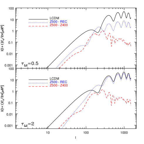
Figure 8: Difference spectra for polarization. In the upper panel $\tau_{{}_{\rm LiI}}=0.5$ and in the lower panel $\tau_{{}_{\rm LiI}}=2.0$.

The power spectra of the difference maps, shown in Figure 7 for the temperature and Figure 8 for the $E$–type polarization, are consistent with our interpretation of the cross–correlation spectra between maps. On large scales, the difference between the temperature maps becomes very small. The power in the $Z500$–$Z400$ difference map peaks at $l\sim 450$, while the power for the recombination–$Z500$ difference peaks at $l\sim 250$. The amplitude of the difference increases as the optical depth increases. When $\tau_{{}_{\rm LiI}}$ is large, the difference spectrum for the recombination–$Z500$ polarization almost coincides with that of the primary anisotropies, as a result of the fact that the primary anisotropies dominate over the newly generated ones.

3.3 Comparison to the Far–Infrared Foreground

The main difficulty in measuring the lithium imprint on the CMB anisotropies is the contamination by the far–infrared background (FIB). There has been no detection to date of the anisotropies in this background, and so we have to rely on theoretical estimates (Haiman & Knox 2000; Knox et al. 2001).

In order to properly combine the contributions from the CMB and FIB anisotropies we express intensities in terms of the equivalent Rayleigh–Jeans temperature, $T_{\rm RJ}$ (in $\mu$K). We start by comparing the temperature anisotropies. The total fluctuation amplitude is given by,

$$\Delta T_{\rm RJ}=\Delta T_{\rm RJ}^{\rm CMB}+\Delta T_{\rm RJ}^{\rm FIB}=\Delta T_{\rm RJ}=T_{\rm RJ}^{\rm CMB}\left({\Delta T_{\rm RJ}\over T_{\rm RJ}}\right)_{\rm CMB}+T_{\rm RJ}^{\rm FIB}\left({\Delta T_{\rm RJ}\over T_{\rm RJ}}\right)_{\rm FIB}.$$ (13)

The ratio between the CMB intensity and the central value for the inferred intensity of the FIB (Fixsen et al. 1998; see the central dot–dashed curve in Figure 2 of Haiman & Knox 2000) is of order unity for a lithium scattering redshift $z\sim 500$,

$${T_{\rm RJ}^{\rm CMB}\over T_{\rm RJ}^{\rm FIB}}\approx\left({500\over 1+z}\right)\exp\left\{15.78\left(1-{500\over 1+z}\right)\right\}.$$ (14)

As noted by Loeb (2001), the temperature fluctuations in the Wien tail translate to intensity fluctuations, $DeltaI_{\nu}$ (in ${\rm erg~{}s^{-1}cm^{-2}sr^{-1}Hz^{-1}}$), of a much larger contrast,

$$\left({\Delta T_{\rm RJ}\over T_{\rm RJ}}\right)_{\rm CMB}\equiv{\Delta I_{\nu}\over I_{\nu}}=\left({d\ln I_{\nu}\over d\ln T}\right){\Delta T\over T}=\left({h\nu\over kT}\right){\Delta T\over T}=15.78\times\left({500\over 1+z}\right){\Delta T\over T}~{}~{},$$ (15)

where we have substituted $I_{\nu}(T)\propto\exp(-h\nu/kT)$ and $T=2.725$ K (Mather et al. 1999). The anisotropy amplitude shown in Figure 7 depends on $\tau_{{}_{\rm LiI}}$, but roughly implies $(\Delta T_{\rm RJ}/T_{\rm RJ})_{\rm CMB}\sim 3\times 10^{-4}[500/(1+z)]$. Haiman & Knox (2000) and Knox et al. (2001) estimate, $(\Delta T_{\rm RJ}/T_{\rm RJ})_{\rm FIB}=0.05$–$0.1$. The FIB anisotropies peak at an $l$ of a few hundred but the peak is very broad. The anisotropies in the FIB are relatively large since they originate from clustering of sources at low redshifts, $z\sim 1$.

We conclude that if $50\%$ of the lithium ions recombine at $z\sim 500$ then

$${\Delta T_{\rm RJ}^{\rm CMB}\over\Delta T_{RJ}^{\rm FIB}}\approx 3\times 10^{-3}\left({500\over 1+z}\right)^{2}\exp\left\{15.78\left(1-{500\over 1+z}\right)\right\}.$$ (16)

Since the CMB contribution is sub-dominant, it is essential to exploit the different frequency dependence of the FIB and CMB anisotropies in order to subtract the FIB contribution with high precision. This might be possible on small angular scales, where the temperature anisotropies generated by lithium scattering at different redshifts are uncorrelated, as indicated by Figures 5 and 7. Also, since the FIB is produced by point sources, observations with high angular resolution can resolve the sources and remove them individually.

Next we consider polarization. While the intensity anisotropies of the FIB are dominated by the clustering of the sources rather than by Poisson fluctuations, the situation is different for the polarization anisotropies. We assume that each source is polarized with a degree of polarization $\epsilon$, and that the polarizations of different sources are uncorrelated. Under these assumptions, it is easy to show that both the $E$ and $B$–polarization spectra share the same amplitude of

$$\epsilon^{2}/2\times C_{Tl}^{\rm Poisson},$$ (17)

where $C_{Tl}^{\rm Poisson}$ is the Poisson contribution to the temperature anisotropies. The Poisson fluctuations can be calculated based on the SCUBA source counts, and are shown as the light solid line in Figure 3 of Haiman & Knox (2000).

The Poisson component of the FIB anisotropies is approximately a factor of $\sim 100$ smaller in power than the total temperature anisotropies at $l\sim 100$–$200$. If we adopt an average value of $\epsilon=0.4\%$ (Jones 1993), then the $E$–polarization is lower by a factor $(0.4\%/\sqrt{2})\times 0.1=2.8\times 10^{-4}$ than the intensity fluctuations.

On the other hand, Figures 2 and 4 imply that the CMB is approximately 10 % polarized for $l\gtrsim 200$. We therefore get that as long as lithium recombines around $z\sim 500$,

$${\Delta E_{\rm RJ}^{\rm CMB}\over\Delta E_{\rm RJ}^{\rm FIB}}\approx 1.1\times\left({\epsilon\over 0.4\%}\right)\left({500\over 1+z}\right)^{2}\exp\left\{15.78\left(1-{500\over 1+z}\right)\right\}.$$ (18)

A property which could be very useful in experimental attempts to isolate the signal is that the polarization signature due to lithium has only an $E$–type component, while the FIB polarization has an equal amplitude in both the $E$ and $B$–type components. The $B$–type polarization could therefore be used to monitor the FIB contamination and could play an essential role in the subtraction of the FIB.

Depending on the nature of the sources responsible for the FIB and their luminosity function it may eventually become possible to resolve most of the FIB through high–resolution observations at different wavelengths. This approach is used, for example, in observational studies of the Sunyaev–Zeldovich effect, where much of the contribution from discrete foreground sources is subtracted out through deep, high–resolution observations at either radio or optical–infrared wavelengths. At the present time there are no available source counts in the wavelength range we consider here. Closest in wavelength are source counts from the SCUBA instrument (see, e.g. Fig. 2 in Borys et al. 2000). If most of the FIB could be resolved, the task of detecting the effect of lithium would become easier as the overall level of contamination would be drastically reduced. Future studies of the FIB will determine whether this reduction is feasible.

4 Conclusions

We have shown that if more than half of the lithium ions recombine by $z\sim 500$, then the temperature and polarization anisotropies of the CMB would be strongly altered at an observed wavelength of $335\mu$m (see Figs. 2 and 4). For high multipoles $l\gg 10$, the change is dominated by two contributions: (i) the Doppler anisotropies induced at the sharp lithium scattering surface; and (ii) the uniform $\exp\{-\tau_{{}_{\rm LiI}}\}$ suppression of the primary anisotropies which were generated at hydrogen recombination (decoupling). Maps taken at wavelengths that are different by only $\sim 10\%$ are expected to have significant differences (see Figs. 7 and 8).

The above signals are superimposed on top of the far infrared background (FIB). Our estimates imply that the lithium imprint on the CMB polarization should be comparable to that provided by the FIB (Eq. 18). Detection is more difficult for the temperature anisotropies (Eq. 16).

The wavelength range we explored overlaps with the highest frequency channel of the Planck mission ($352\mu$m) and with the proposed balloon–borne Explorer of Diffuse Galactic Emissions (EDGE) which will survey 1% of the sky in 10 wavelength bands between $230$–$2000\mu$m with a resolution ranging from $6^{\prime}$ to $14^{\prime}$ (see Table 1 in Knox et al. 2001). In order to optimize the detection of the lithium signature on the CMB anisotropies, a new instrument design is required, with multiple narrow bands ($\Delta\lambda/\lambda\lesssim 0.1$) at various wavelengths in the range $\lambda=250$–$350\mu$m. The experiment should cover a sufficiently large area of the sky so as to determine reliably the statistics of fluctuations on degree scales. In order to minimize contamination from the FIB, the detector should be sensitive to polarization. For reference, the experiment should also measure the anisotropies at shorter wavelengths where the FIB dominates. In order to detect the effect of lithium, high signal-to-noise maps of the primordial CMB should be made for the same region of the sky. Most likely, those maps will become available from future CMB missions such as Planck. A strategy for eliminating the contribution from the brightest FIB sources may also be needed.

The resonant optical depth depends sensitively on the primordial lithium abundance and the recombination history of lithium. More detailed calculations of lithium recombination will be done in a forthcoming paper (Dalgarno, Loeb, & Stancil 2001). Detection of the lithium signature will also allow to calibrate the primordial lithium abundance, which is a sensitive indicator of the mean value and the clumpiness in the baryon abundance during Big Bang nucleosythesis. The lithium abundance in nearby stars is subject to large astrophysical uncertainties (Burles et al. 2001, and references therein). We note that values of the lithium opacity which are higher than the ones we have used, are potentially possible. As an extreme example, lithium abundance values as high as $X_{\rm LiI}\sim 10^{-8}$ were suggested by models of inhomogeneous Big–Bang nucleosynthesis (Applegate & Hogan 1985; Sale & Mathews 1986; Mathews et al. 1990),

The lithium signature on the CMB anisotropies provides the only direct probe of structure in the universe at a redshift $z\sim 400$–500. This redshift marks the beginning of the “dark ages” which end only after the first generation of galaxies form at $z\sim 20$ (see review by Barkana & Loeb 2001).

References

- Applegate & Hogan (1985) Applegate, J. H. & Hogan, C. J. 1985, Phys. Rev. D, 31, 3037
- (2) Barkana, R., & Loeb, A. 2001, Physics Reports, in press; astro-ph/0010468
- (3) Borys, C. et al. 2000; astro-ph/0009143
- (4) Burles, S., Nollett, K. M., & Turner, M. S. 2001, ApJ, in press; astro-ph/0010171
- (5) Chandrasekhar, S. 1960, Radiative Transfer, (New-York: Dover), pp. 50-53
- (6) Dalgarno, A., Loeb, A., & Stancil, P. 2001, in preparation
- Fixsen et al. (1998) Fixsen, D. J., Dwek, E., Mather, J. C., Bennett, C. L., & Shafer, R. A. 1998, ApJ, 508, 123
- (8) Halverson, N. W. et al. 2001; astro-ph/0104489
- (9) Hamilton, D. R. 1947, ApJ, 106, 457
- Jones (1993) Jones, T. J. 1993, ApJ, 403, 135
- (11) Knox, L, Cooray, A., Eisenstein, D., & Haiman, Z. 2001, ApJ, 550, 7
- Haiman & Knox (2000) Haiman, Z. & Knox, L. 2000, ApJ, 530, 124
- (13) Lee, A. T. et al. 2001; astro-ph/0104459
- (14) Loeb, A. 2001, ApJL, in press; astro-ph/0103505
- Ma & Bertschinger (1995) Ma, C. P. & Bertschinger, E. 1995, ApJ, 455, 7
- Mather et al. (1999) Mather, J. C., Fixsen, D. J., Shafer, R. A., Mosier, C., & Wilkinson, D. T. 1999, ApJ, 512, 511
- Mathews, Alcock, & Fuller (1990) Mathews, G. J., Alcock, C. R., & Fuller, G. M. 1990, ApJ, 349, 449
- (18) Netterfield, C. B. et al. 2001; astro-ph/0104460
- Palla, Galli, & Silk (1995) Palla, F., Galli, D., & Silk, J. 1995, ApJ, 451, 44
- Sale & Mathews (1986) Sale, K. E. & Mathews, G. J. 1986, ApJL, 309, L1
- Seljak & Zaldarriaga (1996) Seljak, U. & Zaldarriaga, M. 1996, ApJ, 469, 437
- Smith, Kawano, & Malaney (1993) Smith, M. S., Kawano, L. H., & Malaney, R. A. 1993, ApJS, 85, 219
- (23) Sobolev, V. V. 1946, Moving atmospheres of Stars (Leningrad: Leningrad State University [in Russian]; English translation: 1960 (Cambridge: Harvard Univ. Press)
- (24) Stancil, P. C., Lepp, S., & Dalgarno, A. 1996, ApJ, 458, 401
- (25) —————————————————–. 1998, ApJ, 509, 1
- Stenflo (1980) Stenflo, J. O. 1980, A&A, 84, 68
- (27) Yu, Q., Spergel, D. N., & Ostriker, J. P. 2001, ApJ, submitted, astro-ph/0103149
- Walker et al. (1991) Walker, T. P., Steigman, G., Kang, H., Schramm, D. M., & Olive, K. A. 1991, ApJ, 376, 51
- Zaldarriaga & Harari (1995) Zaldarriaga, M. & Harari, D. D. 1995, Phys. Rev. D 52, 3276
- Zaldarriaga, Spergel, & Seljak (1997) Zaldarriaga, M., Spergel, D. N., & Seljak, U. 1997, ApJ, 488, 1
- Zaldarriaga (1997) Zaldarriaga, M. 1997, Phys. Rev. D 55, 1822