Structure of Small-Scale Magnetic Fields in the Kinematic Dynamo Theory

Abstract

A weak fluctuating magnetic field embedded into a turbulent conducting medium grows exponentially while its characteristic scale decays. In the interstellar medium and protogalactic plasmas, the magnetic Prandtl number is very large, so a broad spectrum of growing magnetic fluctuations is excited at small (subviscous) scales. The condition for the onset of nonlinear back reaction depends on the structure of the field lines. We study the statistical correlations that are set up in the field pattern and show that the magnetic-field lines possess a folding structure, where most of the scale decrease is due to the field variation across itself (rapid transverse direction reversals), while the scale of the field variation along itself stays approximately constant. Specifically, we find that, though both the magnetic energy and the mean-square curvature of the field lines grow exponentially, the field strength and the field-line curvature are anticorrelated, i.e., the curved field is relatively weak, while the growing field is relatively flat. The detailed analysis of the statistics of the curvature shows that it possesses a stationary limiting distribution with the bulk located at the values of curvature comparable to the characteristic wave number of the velocity field and a power tail extending to large values of curvature where it is eventually cut off by the resistive regularization. The regions of large curvature, therefore, occupy only a small fraction of the total volume of the system. Our theoretical results are corroborated by direct numerical simulations. The implication of the folding effect is that the advent of the Lorentz back reaction occurs when the magnetic energy approaches that of the smallest turbulent eddies. Our results also directly apply to the problem of statistical geometry of the material lines in a random flow.

PACS number(s): 47.27.Gs, 98.35.Eg, 47.65.+a, 05.10.Gg

Published in Phys. Rev. E, vol. 65, article 016305 (2002)

I Introduction

It was demonstrated by Batchelor [1] that a weak magnetic field passively advected by a turbulent velocity field would grow, while its characteristic scale would decay. If the magnetic Prandtl number (the ratio of fluid viscosity $\nu$ and magnetic diffusivity $\eta$, ${\rm Pr}=\nu/\eta$) is large, there is a broad range of subviscous scales available to magnetic fluctuations, but not to fluid motions. This physical situation is realized in such astrophysical environments as the interstellar medium and protogalactic plasmas, where ${\rm Pr}$ ranges between $10^{14}$ and $10^{22}$, which provides for $7$ to $11$ decades of subviscous range. The weak-field (kinematic) regime is believed to represent the initial stage of the formation of the currently observed magnetic fields of galaxies. These fields, which possess a coherent large-scale component and whose energies are comparable to the energies of fluid motions of the interstellar medium [2, 3, 4], are thought to have originated from very weak initial seed fields in the galaxies (or protogalaxies), which have been amplified and brought to their current strength and configuration by the dynamo action of the (proto)galactic turbulent plasmas (see Refs. [5, 6] and references therein). Constructing a definitive and quantitative theory of this process remains an open problem. This theory must necessarily be a nonlinear one, because the observed fields are not weak. However, developing such a nonlinear theory of the magnetic-field evolution will require a thorough understanding of its linear (kinematic) precursor. In fact, this point holds with greater force in view of the recent theoretical and numerical advances which suggest that the saturated spectra of magnetic fluctuations are largely determined by the turbulent advection processes that drive the kinematic dynamo [7, 8, 9]. In this work, we study the geometrical structure of the fluctuating small-scale magnetic fields produced by the kinematic stage of the high-${\rm Pr}$ dynamo. Our findings will have direct bearing on such issues as the condition for the onset of nonlinear effects, the geometry of the field as it enters the nonlinear stage of its evolution, and the feasibility of transfering the small-scale magnetic fluctuation energy to larger-scale components of the field.

In an ideal (or highly-conducting) fluid, the magnetic fields are (nearly) frozen into the ambient flow. Therefore, besides being important for the astrophysical dynamo as outlined above, studying passive advection of the magnetic field is equivalent to studying the statistics of stretching and distortion of material lines by random flows, which is a fundamental problem in the theory of turbulence [10]. This subject has attracted considerable attention [10, 11, 12, 13, 14, 15, 16, 17, 18, 19, 20, 21]. Our results on the statistical geometry of magnetic-field lines will have direct applicability in this area. For the sake of unity of exposition, we will proceed to develop our theory in the language of the kinematic-dynamo problem and relegate the drawing of the parallels with the problem of material-line advection to the end of the discussion section, which concludes this work (Sec. IV).

The mathematical formulation and treatment of the small-scale kinematic-dynamo problem were initiated by Kazantsev [22]. Kulsrud and Anderson [23] developed a detailed spectral theory of the small-scale magnetic fluctuations. (A comprehensive exposition of the modern state of the second-order statistical theory of the small-scale kinematic dynamo with large Prandtl numbers, as well as the generalization of Kazantsev’s and Kulsrud and Anderson’s theories to the case of arbitrarily compressible velocity fields, can be found in Ref. [6].) It was established that the characteristic scale of the advected magnetic field decreases exponentially fast at a rate comparable to that of the field growth. The magnetic spectrum quickly shifts its bulk toward scales extremely small compared to those of the velocity field. The decrease of the characteristic scale is checked only by the Ohmic resistive dissipation. Such a regime persists as long as the kinematic approximation remains valid.

It is interesting, and, in fact, necessary for a variety of applications, to inquire what those small-scale fields “look like”: do they really tangle into a completely chaotic and fine-scaled web? The most important reason for such an inquiry is that it is the structure, not just the strength, of the small-scale magnetic fields that determines the conditions for the onset of the nonlinear regime. Indeed, we observe that the Lorentz tension force ${\bf B}\cdot\nabla{\bf B}$ only involves the parallel gradient of the magnetic field [24]. Heuristically, the nonlinear Lorentz feedback will start to play an important role when the Lorentz tension force becomes comparable to inertial terms in the hydrodynamic momentum equation, namely, when $B^{2}\sim(k_{\nu}/k_{\parallel})\rho u^{2}$, where ${\bf u}$ is the velocity field, $k_{\nu}$ is the smallest-eddy wave number, $\rho$ is the density of the medium, and $k_{\parallel}$ is the characteristic wave number of the magnetic-field variation along itself. For chaotically tangled fields, the ratio $k_{\nu}/k_{\parallel}$ can be as small as $k_{\nu}/k_{\eta}\sim{\rm Pr}^{-1/2}$, where $k_{\eta}$ is the resistive-regularization wave number. The kinematic stage of the dynamo will then only produce very weak small-scale fields. On the other hand, if $k_{\parallel}$ is restricted from growing to be as large as $k_{\eta}$, the kinematic dynamo can drive small-scale magnetic fluctuations of energies approaching that of the smallest turbulent eddies. Much of the previous work on the small-scale dynamo and such issues as ambipolar damping and viscous relaxation of small-scale magnetic fluctuations was based on specific assumptions about the magnitude of $k_{\parallel}$ [23, 25, 26]. Understanding the structure of the magnetic field, and, in particular, the statistics of the field-line curvature, is also crucial for the study of the effect of the Braginskii tensor viscosity [27] on the small-scale magnetic fields [28, 29].

FIG. 1.: Stretching of magnetic-field lines by a linear shear flow.

It was suggested by Cowley [30] on intuitive grounds and later supported by numerical simulations [7, 8, 9] that a large-scale advecting field, which is locally just a linear shear flow, could only stretch the magnetic field and make it flip direction ever more rapidly in the plane transverse to the field itself [see Fig. 1 and Fig. 3(a)]. It was argued that no appreciable change of the characteristic scales at which the magnetic field varies along itself could, therefore, be produced. In other words, the exponential increase of the typical fluctuation wave number $k=(k_{\perp}^{2}+k_{\parallel}^{2})^{1/2}$ is expected to be due mostly to the increase of $k_{\perp}$ (rapid transverse direction reversals), while $k_{\parallel}$ stays approximately unchanged, so $k_{\perp}\gg k_{\parallel}\sim k_{\nu}$. Such folding nature of the small-scale fields is consistent with the predominance of volume deformations with greatly disparate spatial dimensions, which is a well known fact in the the theory of kinematic dynamo and passive advection [31, 32]. It is also, of course, directly related to the extreme flux-cancellation property (fine-scale spatial oscillation of field orientation) of the dynamo-generated magnetic fields in maps and chaotic flows extensively studied by Ott and coworkers (see review [33] and references therein) and by Cattaneo [34].

In this paper, we construct an explicit statistical description of the folding effect in the small-scale kinematic-dynamo theory and study the correlations that are set up between the curvature of the magnetic-field lines and the strength of the magnetic field. Since we are interested in the geometrical properties of the field, we neglect the resistive effects present at extremely small scales and consider the diffusion-free induction equation

$${{\rm d}\over{\rm d}t}\,{\bf B}={\bf B}\cdot\nabla{\bf u}-{\bf B}\nabla\cdot{\bf u},$$ (1)

where ${{\rm d}\over{\rm d}t}\,={\partial_{t}}+{\bf u}\cdot\nabla$ is the full convective derivative, ${\bf B}(t,{\bf x})$ is the passive magnetic field and ${\bf u}(t,{\bf x})$ is the externally prescribed velocity field. Let us introduce an auxiliary field ${\bf F}={\bf B}\cdot\nabla{\bf B}$, which is, of course, the magnetic-tension part of the Lorentz force. It is readily seen that ${\bf F}(t,{\bf x})$ evolves according to the following equation

$${{\rm d}\over{\rm d}t}\,{\bf F}={\bf F}\cdot\nabla{\bf u}-2{\bf F}\nabla\cdot{\bf u}+{\bf B}{\bf B}:\nabla\nabla{\bf u}-{\bf B}{\bf B}\cdot\nabla\nabla\cdot{\bf u}.$$ (2)

Let us first describe a very simple semiquantitative argument that supports the folding picture. In the incompressible case ($\nabla\cdot{\bf u}=0$), we notice that the evolution equation (2) for the Lorentz tension force ${\bf F}$ is identical to that for the magnetic field with the exception of the term ${\bf B}{\bf B}:\nabla\nabla{\bf u}$, which contains second derivatives of the velocity field. Suppose that an initial distribution of the small-scale magnetic fluctuations has been set up in such a way that its characteristic parallel and perpendicular wave numbers are comparable and both are much greater than the characteristic wave number of the velocity field: $k_{\parallel}\sim k_{\perp}\gg k_{\nu}$. Then the second derivatives of the velocity field can be neglected and the mean-square tension force ${\langle F^{2}\rangle}$ must grow in the same way as the magnetic energy ${\langle B^{2}\rangle}$. For the characteristic wave number of the magnetic field we then have

$${\overline{k_{\parallel}^{2}}}\sim{{\langle F^{2}\rangle}\over{\langle B^{4}\rangle}}\propto{{\langle B^{2}\rangle}\over{\langle B^{4}\rangle}}<{\rm const}\,e^{-\gamma_{2}t},$$ (3)

where $\gamma_{2}$ is the growth rate of the magnetic energy ${\langle B^{2}\rangle}$ and we have used the obvious fact that ${\langle B^{4}\rangle}\geq{\langle B^{2}\rangle}^{2}$. Thus, any initial field arrangement where magnetic-field lines are chaotically tangled will decay toward a folding state at the rate comparable to the rate of the magnetic energy growth [cf. Fig. 4(a)].

In order to see how the situation develops when ${\overline{k_{\parallel}^{2}}}$ becomes comparable to $k_{\nu}^{2}$, a more complete analysis of the statistics of the magnetic field and the Lorentz tension is required. In Sec. II, we we carry out such an analysis exactly for the case of incompressible velocity field, and prove that ${\overline{k_{\parallel}^{2}}}={\langle F^{2}\rangle}/{\langle B^{4}\rangle}$ stabilizes at a value $\sim k_{\nu}^{2}$. We then take up the question of the evolution of the magnetic curvature, which was recently raised by Malyshkin [35]. We confirm Malyshkin’s result on the exponential growth of the mean-square curvature. Most importantly, we find that, while the ratio of averages ${\langle F^{2}\rangle}/{\langle B^{4}\rangle}$ tends to a constant, the averaged ratio ${\langle F^{2}/B^{4}\rangle}$ follows the exponential growth of the mean-square curvature. This discrepancy implies that the magnetic-field strength and the curvature of the magnetic-field lines are very strongly anticorrelated, i.e., the magnetic field is weak wherever the curvature is large, and vice versa. The picture of folded magnetic-field lines is manifestly consistent with this property, while that of chaotically tangled ones is not. We argue that the large values of curvature in the bends of the folds account for the overall growth of the mean-square curvature, even though these bends occupy only a small fraction of the total volume of the system. At the end of Sec. II, we present a simple qualitative description of the folded-magnetic-field-line geometry that makes possible the statistical correlations we have found.

In Sec. III, we undertake a more detailed study of the one-point distribution of the magnetic-field-line curvature and derive equations for its probability density function (PDF) and all of its moments. This is necessary in order to prove the statement of Sec. II that the curvature only grows exponentially in a small fraction of the total volume of the system. We discover that, while the moments of the curvature diverge exponentially in time, its distribution tends to a stationary limiting profile whose bulk is concentrated at the values of curvature $\sim k_{\nu}$ and which has a power tail at large values of curvature (the exponent is $-13/7$ in the 3D incompressible case). We conclude that the fraction of the volume where the growth of the curvature takes place tends to zero with time. The limiting values of the curvature moments are determined by the resistive regularization at the scales where the magnetic diffusivity becomes important: $k_{\eta}\sim{\rm Pr}^{1/2}k_{\nu}$.

Our theoretical results on the folding structure of the magnetic field, the anticorrelation between the field strength and the field-line curvature (Sec. II), the growth of the curvature moments, and the stationary limiting distribution of the curvature (Sec. III) are backed up by the numerical evidence based on the 3D incompressible MHD simulations by Maron and Cowley [9]. The relevant numerical results are reported at the end of each section. The agreement between our theory and direct numerical simulations of a realistic MHD environment is quite remarkable, especially in view of the idealized character of our modeling assumptions.

In Sec. IV, we summarize our findings and discuss the implications for the nonlinear dynamo theory. The fundamental consequence of the folding effect (i.e., of the fact that the parallel scale of the small-scale magnetic fields does not decay) is that the nonlinear regime sets in only when the magnetic energy becomes comparable to the energy of the smallest turbulent eddies. We also explain how our results apply to the problem of statistical geometry of material lines in isotropic turbulence and relate our conclusions to the previous work on this subject. Numerical results obtained by several authors in this context provide further confirmation of our theory. The fact that the same set of basic features of the curvature statistics is found in a number of different approaches and models, many of them much more realistic than ours, indicates that these statistics may have a largely universal character.

The paper also includes three appendices. In Appendix A, we explain the technical details of the derivation of the Fokker-Planck equations used in the paper. Appendix B is devoted to the study of the structure of the small-scale magnetic fields for the case of advecting flows that possess an arbitrary degree of compressibility. We find that the folding effect as described above only persists as long as the degree of compressibility of the flow remains below a certain critical value. Once this value is exceeded, both the parallel and the perpendicular scales of the magnetic-field variation decay exponentially fast (albeit at different rates) into the subviscous scale range and towards the resistive scales. If this decay continues until the parallel and the perpendicular scales are equalized, the folding pattern is replaced by the tangled one. However, the tangled state is only set up in a small fraction of the total volume where the density of the medium is high and where most of the magnetic-field growth takes place. In the larger (and less dense) part of the system, the magnetic field stays relatively weak and flat. This new situation brought about by compressibility is due to the ability of compressible flows to shrink volumes of the medium with frozen-in magnetic-field lines. The structure of the field is determined by the competition between stretching and contraction. In Appendix C, the above consideration of the compressibility effects is related to the general theory of passive advection in compressible flows developed in Ref. [32].

II Statistics of Lorentz Tension and Magnetic-Field-Line Curvature

In this section, we will restrict our consideration to the case of incompressible velocity field. The evolution equations for the magnetic field ${\bf B}(t,{\bf x})$ and the Lorentz tension ${\bf F}(t,{\bf x})$ in this case are obtained from the equations (1) and (2) by setting $\nabla\cdot{\bf u}=0$. As is customary in the problems of passive advection [36, 12] and kinematic dynamo [22], we choose the advecting velocity ${\bf u}(t,{\bf x})$ to be a Gaussian white-noise-like random field (the Kazantsev-Kraichnan flow), whose statistics are defined by its second-order correlation tensor

$$\left\langle u^{i}(t,{\bf x})u^{j}(t^{\prime},{\bf x}^{\prime})\right\rangle=\delta(t-t^{\prime})\kappa^{ij}({\bf x}-{\bf x}^{\prime}).$$ (4)

As we will only have to deal with one-point statistical quantities, all the relevant information about the velocity correlation properties is contained in the Taylor expansion of $\kappa^{ij}$ around the origin [37]

$$\kappa^{ij}({\bf y})=\kappa_{0}\delta^{ij}-{1\over 2}\,\kappa_{2}\bigl{[}y^{2}\delta^{ij}+2ay^{i}y^{j}\bigr{]}+{1\over 4}\,\kappa_{4}y^{2}\bigl{[}y^{2}\delta^{ij}+2by^{i}y^{j}\bigr{]}+\cdots,$$ (5)

as $y\to 0$. In order to ensure incompressibility, we must set $a=-1/(d+1)$ and $b=-2/(d+3)$, where $d$ is the dimension of space. Our consideration is formally in $d$ dimensions, so that both the two- and the three-dimensional cases can be considered in a unified framework.

The fields ${\bf B}(t,{\bf x})$ and ${\bf F}(t,{\bf x})$ satisfy a a closed system of equations, and, in order to study their statistical properties, we derive the Fokker-Planck equation for the joint PDF of ${\bf B}(t,{\bf x})$ and ${\bf F}(t,{\bf x})$ at an arbitrary fixed point ${\bf x}$. Due to the homogeneity of the problem, this one-point PDF $P(t;{\bf B},{\bf F})$ is independent of ${\bf x}$. A standard derivation procedure explained in Appendix A leads to the following equation for $P$:

$${\partial_{t}}P=-{1\over 2}\,\kappa^{ij}_{,kl}\left({\partial\over\partial B^{i}}B^{k}+{\partial\over\partial F^{i}}F^{k}\right)\left({\partial\over\partial B^{j}}B^{l}+{\partial\over\partial F^{j}}F^{l}\right)P+{1\over 2}\,\kappa^{ij}_{,klmn}{\partial^{2}\over\partial F^{i}\partial F^{j}}B^{k}B^{l}B^{m}B^{n}P.$$ (6)

The indices following a comma in the subscripts always mean spatial derivatives: ${}_{,k}={\partial/\partial x^{k}}$. $\kappa^{ij}_{,kl}$ and $\kappa^{ij}_{,klmn}$ are the tensors of second and fourth derivatives, respectively, of the velocity correlator $\kappa^{ij}({\bf y})$ taken at ${\bf y}=0$. The derivatives with respect to $B^{i}$ and $F^{i}$ in Eq. (6) act rightwards on all terms they multiply. The Einstein convention of summing over repeated indices is used throughout. Eq. (6) contains all the one-point statistical information about the distribution of ${\bf B}$ and ${\bf F}$ and can, therefore, be employed to calculate any individual or mixed averages of these quantities. This is done by multiplying Eq. (6) through by the quantity whose average is sought and integrating both sides with respect to ${\bf B}$ and ${\bf F}$. The derivatives are removed via integration by parts and an ordinary differential equation is established for the desired average, whose time derivative is thereby linked to a linear combination of other averages (including itself). The latter averages must in turn be calculated in the same fashion. We will see that in many cases of interest, very simple linear equations or closed systems of linear equations emerge.

Let us start by calculating the mean-square Lorentz tension. We get

$${\partial_{t}}{\langle F^{2}\rangle} = \gamma_{F}{\langle F^{2}\rangle}+S_{F}{\langle B^{4}\rangle},$$ (7)

$${\partial_{t}}{\langle B^{4}\rangle} = \gamma_{4}{\langle B^{4}\rangle}.$$ (8)

The expressions for the coefficients $\gamma_{F}$, $S_{F}$, $\gamma_{4}$, as well as for others that will arise in what follows, are collected in Table I. Note that, in accordance with the simple argument we described in the Introduction, the growth rate $\gamma_{F}$ of ${\langle F^{2}\rangle}$ is the same as that of the magnetic energy ${\langle B^{2}\rangle}$: $\gamma_{F}=\gamma_{2}$.

Coefficient	Expression	Incompressible		Irrotational
		$d=3$	$d=2$	$d=3$	$d=2$
Compressibility parameters
$a$	see expansion (5)	-1/4	-1/3	1	1
$b$	see expansion (5)	-1/3	-2/5	2	2
$\beta$	$d[1+(d+1)a]$	0	0	15	8
$\zeta$	$d[2+(d+3)b]$	0	0	42	24
Growth rates (from first derivatives of ${\bf u}$)
$\gamma_{2}/\kappa_{2}$	$${d-1\over d+1}\left(d+2+\beta\right)$$	5/2	4/3	10	4
$\gamma_{4}/\kappa_{2}$	$$2\,{d-1\over d+1}\left(d+4+3\beta\right)$$	7	4	52	20
$\gamma_{F}/\kappa_{2}$	$${(d-1)(d+2)\over d+1}+{2(3d^{2}-2)\over d(d+1)}\,\beta$$	5/2	4/3	65	28
$\gamma_{K}/\kappa_{2}$	$${(9-d)d-2\over d+1}+{2(5-d)\over d(d+1)}\,\beta$$	4	4	9	12
$\gamma_{M}/\kappa_{2}$	$${d-2\over d+1}\left(d-1+{2\beta\over d}\right)$$	1/2	0	3	0
$\gamma_{MK}/\kappa_{2}$	$${2d\over d+1}\left(1+{\beta\over d^{2}}\right)$$	3/2	4/3	4	4
Source terms (from second derivatives of ${\bf u}$)
$S_{F}/\kappa_{4}$	$$\bigl{[}6(d+4)+\zeta\bigr{]}{d-1\over d+3}$$	14	36/5	28	12
$S_{K}/\kappa_{4}$	$$6(d-1)$$	12	6	12	6
$S_{M}/\kappa_{4}$	$$\left(6+\zeta\right){d-1\over d+3}$$	2	6/5	16	6

TABLE I.: Coefficients for Sec. II. The general formulas listed in this table are for the case of arbitrarily compressible flows (see Appendix B). The results for the incompressible case considered in Sec. II are obtained by setting $\beta=0$ and $\zeta=0$.

Introducing the characteristic parallel wave number of the magnetic fluctuations according to ${\overline{k_{\parallel}^{2}}}={\langle F^{2}\rangle}/{\langle B^{4}\rangle}$, we readily find

$${\overline{k_{\parallel}^{2}}}(t)=\left({\overline{k_{\parallel}^{2}}}(0)-{S_{F}\over\gamma_{4}-\gamma_{F}}\right)e^{-(\gamma_{4}-\gamma_{F})t}+{S_{F}\over\gamma_{4}-\gamma_{F}}\to{S_{F}\over\gamma_{4}-\gamma_{F}}\sim{\kappa_{4}\over\kappa_{2}}\sim k_{\nu}^{2},\quad t\to\infty,$$ (9)

where $k_{\nu}$ is the characteristic wave number of the advecting flow. The exponential decay of ${\overline{k_{\parallel}^{2}}}$ was already captured in the qualitative argument given in the Introduction [see formula (3)]. The existence of a steady limiting solution is due to the presence of the second derivatives of the velocity field in Eq. (2). By taking them into account, we have thus explicitly proved that ${\overline{k_{\parallel}^{2}}}\sim k_{\nu}^{2}$.

Let us now undertake a slightly more detailed analysis of the magnetic-field structure. The Lorentz tension can be decomposed into two orthogonal components

$${\bf F}=B^{2}\left({{\hat{\bf b\mkern-4.0mu}\mkern 4.0mu}{}}\cdot\nabla{{\hat{\bf b\mkern-4.0mu}\mkern 4.0mu}{}}+{{\hat{\bf b\mkern-4.0mu}\mkern 4.0mu}{}}\,{\nabla_{\parallel}B\over B}\right)=B^{2}\left({\bf K}+{\bf M}\right),$$ (10)

where ${{\hat{\bf b\mkern-4.0mu}\mkern 4.0mu}{}}={\bf B}/B$ is the unit vector in the direction of the magnetic field, and $\nabla_{\parallel}={{\hat{\bf b\mkern-4.0mu}\mkern 4.0mu}{}}\cdot\nabla$. The first term is the magnetic curvature vector ${\bf K}={{\hat{\bf b\mkern-4.0mu}\mkern 4.0mu}{}}\cdot\nabla{{\hat{\bf b\mkern-4.0mu}\mkern 4.0mu}{}}$, the second term, ${\bf M}={{\hat{\bf b\mkern-4.0mu}\mkern 4.0mu}{}}\nabla_{\parallel}B/B$, measures the mirror effect and will, for the sake of brevity, be henceforth referred to as the mirror force. Since ${\bf K}\perp{\bf M}$, we have ${\langle F^{2}/B^{4}\rangle}={\langle K^{2}\rangle}+{\langle M^{2}\rangle}$. The mean squares of both of these quantities can be expressed in terms of mixed averages of ${\bf F}$ and ${\bf B}$: ${\langle M^{2}\rangle}={\langle({\bf F}\cdot{\bf B})^{2}/B^{6}\rangle}$ and ${\langle K^{2}\rangle}={\langle F^{2}/B^{4}\rangle}-{\langle({\bf F}\cdot{\bf B})^{2}/B^{6}\rangle}$, which we proceed to calculate with the aid of Eq. (6)

$${\partial_{t}}{\langle K^{2}\rangle} = \gamma_{K}{\langle K^{2}\rangle}+S_{K},$$ (11)

$${\partial_{t}}{\langle M^{2}\rangle} = -\gamma_{M}{\langle M^{2}\rangle}+\gamma_{MK}{\langle K^{2}\rangle}+S_{M}$$ (12)

(see Table I for the values of the coefficients). The exact solution of Eq. (11) is

$${\langle K^{2}\rangle}(t)=\left({\langle K^{2}\rangle}(0)+{S_{K}\over\gamma_{K}}\right)e^{\gamma_{K}t}-{S_{K}\over\gamma_{K}},$$ (13)

so the magnetic curvature grows exponentially (even if it is initially zero). It is instructive to express its growth rate in terms of the growth rate of the magnetic energy ${\langle B^{2}\rangle}$. In three dimensions, this gives $\gamma_{K}=(16/5)\gamma_{2}/2$, which agrees with the result Malyshkin [35] obtained by a direct calculation of ${\langle K^{2}\rangle}$ in the spirit of the Kulsrud-Anderson theory [23]. We also see that the mean-square mirror force [Eq. (12)] is not an independently interesting quantity: after a transient initial time, it is reduced to “mirror” the evolution of the mean-square curvature:

$${\langle M^{2}\rangle}(t)\sim{\gamma_{MK}\over\gamma_{K}+\gamma_{M}}\,{\langle K^{2}\rangle}(t),\quad t\to\infty.$$ (14)

Thus, we have established that, while the ratio of the averages ${\langle F^{2}\rangle}/{\langle B^{4}\rangle}$ tends to a constant value $\sim k_{\nu}^{2}$, the averaged ratio ${\langle F^{2}/B^{4}\rangle}\sim{\langle K^{2}\rangle}\sim e^{\gamma_{K}t}$ grows exponentially. Since both of these quantities have the dimension and the intuitive meaning of some characteristic parallel wave numbers, the question inevitably arises as to the physical interpretation of such drastic dependence on the relative order of the averaging and the normalization with respect to the magnetic-field strength. This dependence clearly indicates that there exists a very strong anticorrelation between the strength of the magnetic field and the curvature of the magnetic-field lines. Namely, while both the mean-square curvature and all moments of $B$ grow exponentially, the magnetic fields are configured in such a way that the magnetic field is very weak wherever its curvature is large, and vice versa. No such arrangement would be possible if the field were chaotically tangled everywhere. Indeed, a tangled state of this sort would imply that the absolute values of the curvature were everywhere comparably large and growing. But then, in order to compensate for the growth of the curvature, the growth of $B^{4}$ would have to be partially or fully suppressed compared to that mandated by Eq. (8).

On the other hand, it is easily envisioned how the strong anticorrelation between $B$ and $K$ can be realized in the folding picture. While the curvature is quite small and magnetic field grows in most of the volume, which is occupied by the folds, the situation is reversed in the small part of the volume where magnetic-field lines bend and reverse direction: the curvature there is very large and magnetic field weak. Fig. 2 illustrates the typical geometry of the folding magnetic-field lines. This picture is in 2D, but can also be interpreted as a cross section of a 3D geometry of a sheetlike configuration. Flux conservation ($\int{\bf B}\cdot{\rm d}{\bf S}=0$) implies ${B_{\rm bend}/B_{\rm fold}}\sim{\ell_{\perp}/\ell_{b}}$, where $\ell_{\perp}$ is the characteristic scale of magnetic-field variation across itself in the folding region and $\ell_{b}$ is the characteristic size of the bend. The velocity shear that produces (or “sharpens”) the bend acts in such a way that $\ell_{\perp}$ is decreased while $\ell_{b}$ is amplified, so $\ell_{b}\gg\ell_{\perp}$, whence $B_{\rm bend}\ll B_{\rm fold}$.

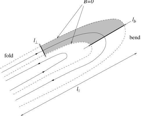
FIG. 2.: The geometry of the folding field lines in the vicinity of the bend. The dashed lines correspond to the surfaces on which the magnetic field vanishes. The shaded area is the cross section of the volume that can be used for the flux-conservation estimate ${B_{\rm bend}/B_{\rm fold}}\sim{\ell_{\perp}/\ell_{b}}$. All the flux is through the surfaces whose cross sections are depicted by the bold lines.

$$\begin{array}[]{cc}\psfig{width=180.67499pt}&\qquad\psfig{width=180.67499pt}\\ &\\ {\rm(a)~{}Magnetic~{}field}~{}B&\qquad{\rm(b)~{}Curvature}~{}K=|{{\hat{\bf b\mkern-4.0mu}\mkern 4.0mu}{}}\cdot\nabla{{\hat{\bf b\mkern-4.0mu}\mkern 4.0mu}{}}|\end{array}$$

FIG. 3.: Instanteneous magnetic-field configuration in the kinematic regime (numerical results). These are greyscale plots of 2D cross sections of the 3D snapshots of (a) the magnetic-field strength and (b) the absolute value of the field-line curvature. These plots are from the same simulation as Fig. 4(b). The field-strength and the curvature snapshots [plots (a) and (b)] are taken at the same moment $t=8.2$ and at the same cross section. Darker regions correspond to larger values of the fields. In the plot (a), $\langle B\rangle\simeq 0.003$, ${\langle B^{2}\rangle}^{1/2}\simeq 0.004$, ${\langle B^{4}\rangle}^{1/4}\simeq 0.006$, and the maximum value of $B$ throughout the system is $\simeq 0.025$. The regions that are pitch black in the plot encompass fields stronger than $0.01$. All of these values correspond to magnetic-field energies well below the nonlinear-saturation threshold. The specific units of the field strength are, of course, of no consequence here. In the plot (b), $\langle K\rangle\simeq 50$, ${\langle K^{2}\rangle}^{1/2}\simeq 70$, $\langle K^{4}\rangle^{1/4}\simeq 110$, and the maximum value of $K$ is $\simeq 520$. The pitch black regions of the plot correspond to curvatures larger than $400$. The curvature has units of inverse length, based on the box size $1$.

It must be recognized, however, that the presence of an anticorrelation between the magnetic-field strength and the magnetic-field-line curvature does not in itself prove that the volume where the growth of the curvature occurs constitutes only a small fraction of the total volume of the system. Indeed, examples of magnetic fields can be constructed that possess such an anticorrelation and where, at the same time, the mean-square curvature grows in any arbitrary fraction of the total volume that can be specified beforehand. Further study of the curvature statistics is, therefore, required to settle this issue. This will be carried out in Sec. III, where the smallness of the volume where the curvature grows is confirmed.

Finally, let us reiterate that the presence of the folding structure has found repeated confirmation by numerical evidence. Most recently, folding was extensively studied in 2D and 3D numerical simulations of the small-scale dynamo effect in a viscosity-dominated MHD model of Kinney et al. [7], and in 3D forced-MHD simulations of Maron and Cowley [9]. Here we present the numerical results that are based on the latter work and directly relate to the theory developed in this section. All numerical results presented in this paper derive from a $128^{3}$ spectral forced-MHD code written by J. Maron and described in detail in Refs. [38, 9]. The external forcing is on the system-size scale and $\delta$ correlated in time. In the simulations quoted in this paper, the hydrodynamic Reynolds numbers are quite small, so the advecting fluid flows are essentially determined by the balance of the forcing and the viscous dissipation. However, this is not really a handicap, as the purpose of the numerical results presented here is to illustrate the kinematic-dynamo properties at subviscous scales. More discussion of this issue can be found in Refs. [7, 8].

$$\begin{array}[]{cc}\psfig{width=234.87749pt}&\psfig{width=234.87749pt}\\ {\rm(a)~{}Decay~{}of}~{}{\langle F^{2}\rangle}/{\langle B^{4}\rangle}~{}(\log_{10}~{}{\rm plot})&\qquad{\rm(b)}~{}{\langle K^{2}\rangle}~{}{\rm and}~{}{\langle F^{2}\rangle}/{\langle B^{4}\rangle}~{}(\log_{10}~{}{\rm plot})\end{array}$$

FIG. 4.: Anticorrelation between the magnetic-field strength and the field-line curvature and growth of the mean-square curvature (numerical results). (a) Time evolution of ${\langle F^{2}\rangle}/{\langle B^{4}\rangle}$ in two simulations where the initial magnetic field is uniformly tangled at subviscous scales. The hollow dots correspond to the simulation with ${\rm Pr}=100$, $k_{\nu}\sim 25$; the filled dots correspond to the simulation with ${\rm Pr}=2500$, $k_{\nu}\sim 5$. (b) Time evolution of ${\langle F^{2}\rangle}/{\langle B^{4}\rangle}$ (hollow dots) and ${\langle K^{2}\rangle}$ (filled dots) in a simulation with the initially flat magnetic field varying transversely at the velocity scales ($k_{\parallel}=0$, $k_{\perp}\sim k_{\nu}$). In this simulation, ${\rm Pr}=2500$, $k_{\nu}\sim 5$, $k_{\eta}\sim 250$. The ratio ${\langle F^{2}\rangle}/{\langle B^{4}\rangle}$ again stabilizes at a value $\sim$ a few times $k_{\nu}^{2}$. In both plots, the quantities plotted have units of inverse length. These are based on the box size $1$. Time is measured in units of the smallest-eddy turnover time $\langle|\nabla\times{\bf u}|^{2}\rangle^{-1/2}$ (in units based on box size $1$ and forcing power $1$, this quantity is $\sim 0.22$).

In Fig. 3, we give the greyscale plots of the magnetic-field strength and the absolute value of the magnetic curvature corresponding to a typical instantaneous magnetic-field configuration observed in a simulated MHD evironment during the kinematic stage of the small-scale dynamo. The folding pattern strikingly similar to the one described above is clearly in evidence (cf. Fig. 2). The anticorrelation between the field strength and the field-line curvature, as well as the intermittent nature of the distribution of both (cf. Sec. III) are also manifest. Fig. 4(a) shows how the ratio ${\overline{k_{\parallel}^{2}}}={\langle F^{2}\rangle}/{\langle B^{4}\rangle}$ adjusts to a stationary value $\sim k_{\nu}^{2}$ from an initial state where the field is chaotically tangled at subviscous scales. We show results of two simulations with such an (artificial) initial field and different values of $k_{\nu}$. In both cases, exponential decay of ${\overline{k_{\parallel}^{2}}}(t)$ toward stationary values $\sim$ a few times $k_{\nu}^{2}$ is observed, which corroborates Eq. (9). Fig. 4(b) portrays the time evolution of the ratio ${\langle F^{2}\rangle}/{\langle B^{4}\rangle}$ and of the mean-square curvature ${\langle K^{2}\rangle}$ in a simulation that starts with the magnetic field concentrated at the velocity scales. The ratio ${\langle F^{2}\rangle}/{\langle B^{4}\rangle}$ again stabilizes at a value $\sim$ a few times $k_{\nu}^{2}$ as predicted by our solution (9). The exponential growth of the mean-square curvature ${\langle K^{2}\rangle}$ proceeds in accordance with our solution (13) until it is checked by the resistive regularization at a stationary value ${\langle K^{2}\rangle}\sim k_{\eta}^{2}$. While our theory was constructed for the diffusion-free regime and, therefore, did not include this effect, the resistive saturation of the curvature is naturally an expected outcome (see Sec. III for more discussion of this issue).

III Distribution of Magnetic-Field-Line Curvature and Magnetic-Field Strength

In the previous section, we indicated the need for a study of the curvature statistics that would go beyond the evolution of the mean square. In this section, we fulfill this program and delve deeper into the detailed properties of the distribution of the magnetic field and its curvature.

The Fokker-Planck equation for the one-point PDF of the magnetic-field-line curvature ${\bf K}={{\hat{\bf b\mkern-4.0mu}\mkern 4.0mu}{}}\cdot\nabla{{\hat{\bf b\mkern-4.0mu}\mkern 4.0mu}{}}$ is most conveniently derived on the basis of the folowing coupled evolution equations for ${\bf K}$ and the magnetic-field direction ${{\hat{\bf b\mkern-4.0mu}\mkern 4.0mu}{}}$:

$${{\rm d}\over{\rm d}t}\,{\bf K} = {\bf K}\cdot(\nabla{\bf u})\cdot({\hat{\mathbb{I}}}-{{\hat{\bf b\mkern-4.0mu}\mkern 4.0mu}{}}{{\hat{\bf b\mkern-4.0mu}\mkern 4.0mu}{}})-{{\hat{\bf b\mkern-4.0mu}\mkern 4.0mu}{}}{\bf K}{{\hat{\bf b\mkern-4.0mu}\mkern 4.0mu}{}}:\nabla{\bf u}-2{\bf K}{{\hat{\bf b\mkern-4.0mu}\mkern 4.0mu}{}}{{\hat{\bf b\mkern-4.0mu}\mkern 4.0mu}{}}:\nabla{\bf u}+{{\hat{\bf b\mkern-4.0mu}\mkern 4.0mu}{}}{{\hat{\bf b\mkern-4.0mu}\mkern 4.0mu}{}}:(\nabla\nabla{\bf u})\cdot({\hat{\mathbb{I}}}-{{\hat{\bf b\mkern-4.0mu}\mkern 4.0mu}{}}{{\hat{\bf b\mkern-4.0mu}\mkern 4.0mu}{}}),$$ (15)

$${{\rm d}\over{\rm d}t}\,{{\hat{\bf b\mkern-4.0mu}\mkern 4.0mu}{}} = {{\hat{\bf b\mkern-4.0mu}\mkern 4.0mu}{}}\cdot(\nabla{\bf u})\cdot({\hat{\mathbb{I}}}-{{\hat{\bf b\mkern-4.0mu}\mkern 4.0mu}{}}{{\hat{\bf b\mkern-4.0mu}\mkern 4.0mu}{}}),$$ (16)

where ${\hat{\mathbb{I}}}$ is the unit dyadic and colons denote double dot products executed according to ${\bf K}{{\hat{\bf b\mkern-4.0mu}\mkern 4.0mu}{}}:\nabla{\bf u}={\bf K}\cdot({{\hat{\bf b\mkern-4.0mu}\mkern 4.0mu}{}}\cdot\nabla{\bf u})$, etc. Both of the above equations are direct corollaries of the induction equation (1). It is easy to see that these equations respect the conservation laws $|{{\hat{\bf b\mkern-4.0mu}\mkern 4.0mu}{}}|=1$ and ${{\hat{\bf b\mkern-4.0mu}\mkern 4.0mu}{}}\cdot{\bf K}=0$. Note that, in this section, we work with arbitrarily compressible velocity fields, so ${\bf u}$ is not required to be divergence-free. It will be seen, however, that none of the essential features of the curvature statistics are affected by the compressibility.

The averaging procedure that leads to the Fokker-Planck equation for the joint PDF $P(t;{\bf K},{{\hat{\bf b\mkern-4.0mu}\mkern 4.0mu}{}})$ does not involve any nonstandard steps and is fully analogous to that used to derive the Fokker-Planck equation (6) (see Appendix A). The result is

$${\partial_{t}}P = -{1\over 2}\,\kappa^{ij}_{,kl}\left(-\delta^{k}_{i}+{\partial\over\partial b^{i}}b^{k}+{\partial\over\partial K^{i}}K^{k}-{\partial\over\partial b^{r}}b^{r}b^{k}b^{i}-2{\partial\over\partial K^{r}}K^{r}b^{k}b^{i}-{\partial\over\partial K^{r}}b^{r}K^{k}b^{i}-{\partial\over\partial K^{r}}b^{r}b^{k}K^{i}\right)$$ (19)

$$\quad\quad\,\,\,\times\left({\partial\over\partial b^{j}}b^{l}+{\partial\over\partial K^{j}}K^{l}-{\partial\over\partial b^{s}}b^{s}b^{l}b^{j}-2{\partial\over\partial K^{s}}K^{s}b^{l}b^{j}-{\partial\over\partial K^{s}}b^{s}K^{l}b^{j}-{\partial\over\partial K^{s}}b^{s}b^{l}K^{j}\right)P$$

$$+\,{1\over 2}\,\kappa^{ij}_{,klmn}\left({\partial\over\partial K^{i}}b^{k}b^{m}-{\partial\over\partial K^{r}}b^{r}b^{k}b^{m}b^{i}\right)\left({\partial\over\partial K^{j}}b^{l}b^{n}-{\partial\over\partial K^{s}}b^{s}b^{l}b^{n}b^{j}\right)P.$$

A major simplification of this equation becomes possible if one recalls that the joint distribution $P(t;{\bf K},{{\hat{\bf b\mkern-4.0mu}\mkern 4.0mu}{}})$ is subject to two constraints: $|{{\hat{\bf b\mkern-4.0mu}\mkern 4.0mu}{}}|=1$ and ${{\hat{\bf b\mkern-4.0mu}\mkern 4.0mu}{}}\cdot{\bf K}=0$. Also taking into account the spatial isotropy of the problem, we conclude that the following factorization holds:

$$P(t;{\bf K},{{\hat{\bf b\mkern-4.0mu}\mkern 4.0mu}{}})=\delta(|{{\hat{\bf b\mkern-4.0mu}\mkern 4.0mu}{}}|^{2}-1)\delta({{\hat{\bf b\mkern-4.0mu}\mkern 4.0mu}{}}\cdot{\bf K})P_{K}(t;K).$$ (20)

The function $P_{K}(t;K)$ is then found to satisfy the following reduced Fokker-Planck equation:

$${\partial_{t}}P_{K} = {1\over 2(d+1)}\,\kappa_{2}\left[\left(5d-1+{6\over d}\,\beta\right)K^{2}P_{K}^{\prime\prime}+\left(11d^{2}-6d+1+{2(7d-2)\over d}\,\beta\right)KP_{K}^{\prime}\right.$$ (22)

$$\left.+\left(d-1\right)\left(2d-1\right)\left(3d-1+{4\over d}\,\beta\right)P_{K}\right]+3\kappa_{4}\left(P_{K}^{\prime\prime}+{d-2\over K}\,P_{K}^{\prime}\right),$$

where primes denote partial derivatives with respect to $K$, the compressibility parameter $\beta=d[1+(d+1)a]$ is nonnegative and vanishes in the incompressible case, and $\kappa_{2}$, $\kappa_{4}$, and $a$ are coefficients of the small-scale expansion (5) of the velocity correlator. Note that the distribution of the curvature is independent of the second compressibility parameter $b$. The normalization rule for $P_{K}(t;K)$ follows from the normalization of the original PDF $P(t;{\bf K},{{\hat{\bf b\mkern-4.0mu}\mkern 4.0mu}{}})$ and from the factorization (20): $(1/2)S_{d}S_{d-1}\int_{0}^{\infty}{\rm d}K\,K^{d-2}P_{K}(t;K)=1$, where $S_{d}=2\pi^{d/2}/\Gamma(d/2)$ is the area of a unit sphere in $d$ dimensions. Absorbing the geometrical prefactor into $P_{K}(t;K)$, we conclude that the true PDF (in the sense that it induces a measure on the volume of the system and integrates to unity) is $K^{d-2}P_{K}(t;K)$. Note that, since the curvature vector must always remain perpendicular to the direction of the magnetic field, the curvature distribution is effectively restricted to $d-1$ dimensions.

It is now straightforward to establish the set of evolution equations for the even moments of the curvature

$${\partial_{t}}\langle K^{2n}\rangle=\left[{2(5d-1)\over d+1}\,n-d+{2\over d}\left({6n\over d+1}-1\right)\beta\right]n\kappa_{2}\langle K^{2n}\rangle+6(d+2n-3)n\kappa_{4}\langle K^{2(n-1)}\rangle,\quad n\geq 1$$ (23)

For $n=1$, Eq. (23) reproduces the results for the mean-square curvature that were obtained in Sec. II and Appendix B [see Eq. (11) and Table I]. The higher moments of the curvature are coupled to the lower ones in a recursive fashion, but also have their own growth rates that increase quadratically with $n$. This latter kind of intermittency is very similar to that encountered in earlier studies of the statistics of the magnetic-field strength [31, 32]. For the sake of comparison, let us list here the Fokker-Planck equation that determines the PDF $B^{d-1}P_{B}(t;B)$ of the magnetic-field strength $B$ and the evolution equation for its moments $\langle B^{2n}\rangle=S_{d}\int_{0}^{\infty}{\rm d}B\,B^{d-1+2n}P_{B}(t;B)$,

$${\partial_{t}}P_{B}={1\over 2}\,\kappa_{2}\,{d-1\over d+1}\,\biggl{[}\left(1+\beta\right)B^{2}P_{B}^{\prime\prime}+(d+1)(1+2\beta)BP_{B}^{\prime}+d(d+1)\beta P_{B}\biggr{]},$$ (24)

$${\partial_{t}}\langle B^{2n}\rangle={d-1\over d+1}\,\bigl{[}2n+d+(2n-1)\beta\bigr{]}n\kappa_{2}\langle B^{2n}\rangle.\qquad\qquad\qquad$$ (25)

The primes in Eq. (24) denote derivatives with respect to $B$. We note that Eq. (8) is a particular case of Eq. (25). Direct derivation of the above equations by averaging the induction equation (1) is quite standard. Details can be found in Ref. [39]. Eq. (24) can also be obtained by integrating out the $F^{i}$ dependence in Eq. (B4) and using the spatial isotropy of the magnetic-field distribution. Eq. (25) is a direct consequence of Eq. (24).

We now turn to the main objective of this section, namely, estimating the fraction of the total volume of the system where the curvature growth occurs. In Eq. (22), denote by $D$, $\Sigma$, and $\Gamma$ the coefficients in front of $K^{2}P_{K}^{\prime\prime}$, $KP_{K}^{\prime}$, and $P_{K}$, respectively. Now rescale time and curvature according to $Dt\Rightarrow t$ and $K/K_{*}\Rightarrow K$, where $K_{*}=(3\kappa_{4}/D)^{1/2}\sim k_{\nu}$ (recall that $k_{\nu}$ is the characteristic wave number of the advecting velocity field). We can now rewrite Eq. (22) in the following nondimensionalized form

$${\partial_{t}}P_{K}=(1+K^{2})P_{K}^{\prime\prime}+\left(\sigma K+{d-2\over K}\right)P_{K}^{\prime}+(d-1)(\sigma-d)P_{K},$$ (26)

where we have used the fact that $\Gamma=(d-1)(\Sigma-Dd)$ and denoted

$$\sigma={\Sigma\over D}={11d^{2}-6d+1+2(7d-2)\beta/d\over 5d-1+6\beta/d}.$$ (27)

Besides the dimension of space, the only essential parameter of the curvature distribution is $\sigma$, which changes with $d$ and the degree of compressibility. The correct boundary conditions for Eq. (26) follow from the normalizability requirement $\int_{0}^{\infty}{\rm d}K\,K^{d-2}P_{K}(t;K)<\infty$,

$$\bigl{[}K^{d-2}P_{K}^{\prime}(t;K)\bigr{]}_{K=0}=0,\qquad\bigl{[}K^{d}P_{K}^{\prime}(t;K)+(\sigma-d)K^{d-1}P_{K}(t;K)\bigr{]}_{K\to\infty}=0.$$ (28)

Let us study the evolution of the curvature statistics from an initial setting where the curvature is zero everywhere: $K^{d-2}P_{K}(t=0,K)\propto\delta(K)$. While such a $\delta$-like initial distribution is, of course, highly artificial, mathematically it is not an anomalous case since, as we have seen [Eq. (23)], the moments of the curvature would grow even from such an initial state. Two distinct asymptotic regimes can be identified in the evolution of the curvature distribution.

Small-curvature regime. For small values of curvature $K\ll 1$ (i.e., for the dimensional curvature much smaller then $K_{*}\sim k_{\nu}$), Eq. (26) reduces to what mathematically is a heat equation in $d-1$ dimensions with radial symmetry

$${\partial_{t}}P_{K}=P_{K}^{\prime\prime}+{d-2\over K}\,P_{K}^{\prime}.$$ (29)

The solution is a heat profile spreading out from the origin

$$P_{K}(t;K)={\rm const}\,{e^{-K^{2}/4t}\over t^{(d-1)/2}}.$$ (30)

Multiplying the solution (30) by $K^{d-2}$, we find the peak of the PDF at $K_{\rm peak}=\sqrt{2(d-2)t}$, i.e., it remains at $K=0$ in 2D and shifts towards larger $K$ in 3D. In either case, the excitation eventually spreads over towards larger $K\sim 1$, where the small-curvature asymptotic regime breaks down.

Large-curvature regime. At large values of curvature $K\gg 1$, the asymptotic form of Eq. (26) is

$${\partial_{t}}P_{K}=K^{2}P_{K}^{\prime\prime}+\sigma KP_{K}^{\prime}+(d-1)(\sigma-d)P_{K}.$$ (31)

In logarithmic variables, this is a 1D diffusion equation with the drift velocity $\sigma-1$ and with an overall growth rate $(d-1)(\sigma-d)$. The corresponding Green’s function is

$$G_{K}(t-t_{0};K,K_{0})={e^{(d-1)(\sigma-d)(t-t_{0})}\over K_{0}\sqrt{4\pi(t-t_{0})}}\,\exp\left(-{\bigl{[}\ln(K/K_{0})+(\sigma-1)(t-t_{0})\bigr{]}^{2}\over 4(t-t_{0})}\right).$$ (32)

Thus, the curvature distribution develops a lognormal tail. This clearly accounts for the intermittency we have detected in the evolution of the curvature moments [Eq. (23)]. Multiplying the Green’s function (32) by $K^{d-2}$, it is not hard to see that the peak of the excitation propagates according to $K_{\rm peak}=K_{0}\exp\bigl{[}(2d-3-\sigma)(t-t_{0})\bigr{]}$. Substituting the value of $\sigma$ [formula (27)], we see that $2d-3-\sigma<0$ in both two and three dimensions, so the peak, in fact, propagates backwards towards smaller values of curvature.

The conclusion from this simple asymptotic analysis is that, after an initial transient time, the curvature PDF should assume the form where its bulk is concentrated at the values of (dimensional) curvature smaller or comparable to $K_{*}\sim k_{\nu}$ and a lognormally decaying tail is formed at $K\gg K_{*}$. The global maximum of the PDF is located at $K=0$ in 2D and at some $K\sim K_{*}$ in 3D. Thus, in most of the volume of the system, the values of the curvature should not greatly exceed $K_{*}$. The growth of the moments of the curvature is, on the other hand, mostly due to the lognormal tail of the distribution. Indeed, multiplying the solutions (30) and (32) by $K^{d-2+2n}$, we see that the relative importance of the small-curvature region decreases, while that of the lognormal tail increases. The peak of the function $K^{d-2+2n}P_{K}(K)$ for $n\geq 1$ always propagates in the forward direction.

Of course, once the solution of Eq. (26) has cleared the region of validity of the small-curvature asymptotic regime, a complicated process of probability redistribution is set up. As time passes, the lognormal tail gains more weight, while the heat profile at small $K$ spreads out. The precise nature of the evolution of the PDF is decided by the interaction between the small-curvature (radial-heat) and large-curvature (lognormal) regimes in the crossover region $K\sim K_{*}$. This interaction can affect the entire PDF. We can gain more insight into what happens by observing that Eq. (26) has a stationary solution. Indeed, let us write Eq. (26) in the following explicitly conservative form:

$${\partial_{t}}P_{K}={1\over K^{d-2}}{\partial\over\partial K}K^{d-2}\left[(1+K^{2})P_{K}^{\prime}+(\sigma-d)KP_{K}\right].$$ (33)

Setting the left-hand side to zero, integrating twice, and making use of the boundary conditions (28) to eliminate one of the constants of integration, we find the following stationary limiting PDF:

$$K^{d-2}P_{K}^{\rm(st)}(K)={\rm const}\,{K^{d-2}\over(1+K^{2})^{(\sigma-d)/2}}.$$ (34)

This PDF satisfies the boundary conditions (28), is properly normalizable, and has a power tail $\sim K^{-[\sigma-2(d-1)]}$. The values of the exponent $\sigma-2(d-1)$ for the incompressible and irrotational cases in two and three dimensions, along with the values of other relevant parameters, are collected in Table II. The curvature distribution can be seen to converge (in the mean-square sense) to the stationary profile (34) if we represent the time-dependent solutions of Eq. (33) in the form $P_{K}(t;K)=C(t;K)P_{K}^{\rm(st)}(K)$ and notice that the prefactor $C(t;K)$ tends to a constant, viz., ${\partial_{t}}\bigl{<}C^{2}\bigr{>}=-2\bigl{<}(1+K^{2})({\partial C/\partial K})^{2}\bigr{>}$, where the averages are with respect to the stationary distribution (34).

Fig. 5 shows the results of numerical solution of Eq. (33) in two and three dimensions for the case of incompressible velocity field. The results for the case of irrotational velocity field are very similar in form (with slightly different power laws at large $K$: see Table II). Collapse of the curvature PDF onto the stationary profile (34) is very quick and proceeds in essentially the same fashion in both incompressible and irrotational cases (see discussion at the end of this section).

$$\begin{array}[]{cc}\psfig{width=234.87749pt}&\psfig{width=234.87749pt}\\ &\\ {\rm(a)}~{}d=2,~{}P_{K}(t;K)&{\rm(b)}~{}d=2,~{}P_{K}(t;K),~{}{\rm ln/ln~{}plot}\\ &\\ \psfig{width=234.87749pt}&\psfig{width=234.87749pt}\\ &\\ {\rm(c)}~{}d=3,~{}KP_{K}(t;K)&{\rm(d)}~{}d=3,~{}KP_{K}(t;K),~{}{\rm ln/ln~{}plot}\end{array}$$

FIG. 5.: The results of a numerical solution of Eq. (26) in two and three dimensions for the case of incompressible velocity field. The numerical solution was initialized with the Gaussian heat profile (30) corresponding to $t=0.2$. Time is measured in the units of $D^{-1}$, curvature in the units of $K_{*}$. We plot the evolving PDF $K^{d-2}P_{K}(t;K)$ (normalized to $1$) at times $t=0.2,0.5,1,2,3,4,5,6,7,8,9$. The PDF that corresponds to the earliest time is the one with the highest peak and the steepest decay at large $K$. At later times, the peak of the PDF descends, while the tail becomes thicker (lognormal with increasing variance and eventually powerlike). The log/log plots (b) and (d) illustrate how the power tail is formed. For the sake of reference, we have also plotted the slopes correspoding to $K^{-[\sigma-2(d-1)]}$ (see Table II).

Velocity Field	Dimension	$\quad a\quad$	$\quad\beta\quad$	$\quad D/\kappa_{2}\quad$	$\quad\Sigma/\kappa_{2}\quad$	$\quad\Gamma/\kappa_{2}\quad$	$\quad\sigma\quad$	$\quad\sigma-2(d-1)\quad$
Incompressible	$d=3$	-1/4	0	7/4	41/4	10	41/7	13/7
	$d=2$	-1/3	0	3/2	11/2	5/2	11/3	5/3
Irrotational	$d=3$	1	15	11/2	34	35	68/11	24/11
	$d=2$	1	8	11/2	43/2	21/2	43/11	21/11

TABLE II.: The coefficients of Eq. (22) and Eq. (26).

$$\begin{array}[]{cc}\psfig{width=234.87749pt}&\psfig{width=234.87749pt}\\ {\rm(a)}~{}d=3,~{}4\pi^{2}KP_{K}(t;K)&\quad{\rm(b)}~{}d=3,~{}4\pi^{2}KP_{K}(t;K),~{}{\rm log_{10}/log_{10}~{}plot}\end{array}$$

FIG. 6.: Curvature PDF from 3D incompressible MHD simulations. This is the same simulation as was used in Fig. 4(b): ${\rm Pr}=2500$, $k_{\nu}\sim 5$, $k_{\eta}\sim 250$, flat initial field. We plot the PDF $4\pi^{2}KP_{K}(t;K)$ (normalized to $1$) at times $t=0.9,1.8,2.7,3.6,4.5,5.5,6.4,7.3$. The curvature has units of inverse length, based on box size $1$. The time is measured in the units of $\langle|\nabla\times{\bf u}|^{2}\rangle^{-1/2}$ (the smallest-eddy turnover time). The PDF that corresponds to the earliest time is the one with the highest peak and the steepest decay at larger $K$. At later times, the peak becomes lower, the decay gentler. (a) is the linear plot, (b) is the log/log plot. The dashed line represents the slope corresponding to $K^{-13/7}$.

An important feature of the stationary PDF (34) is that all the moments $\langle K^{2n}\rangle$ diverge. In the language of physical reality, this means that the limiting values of the curvature moments are essentially determined by the resistive regularization, which must cut off the power tail of the PDF (34) at the scale where magnetic diffusivity becomes important: $k_{\eta}\sim{\rm Pr}^{1/2}k_{\nu}$. This is, of course, hardly surprising because curvature is just a measure of the inverse scale of the magnetic fluctuations and cannot exceed the resistive scale. In view of these findings, the growth rates for the curvature moments that have been obtained in this and the preceding sections, should be interpreted as describing the evolution of the moments while the lognormal tail of the evolving distribution spreads and thickens. The power tail of the stationary limiting distribution (34) forms the envelope inside which this process takes place. In the diffusion-free regime, the stationary distribution itself is attained at $t\to\infty$ with the moments diverging exponentially in time. We should like to observe here that a PDF such as we have obtained, with a power tail and divergent moments, is indicative of a fractal nature of the distribution. It must be clear that the presence and the particular form of the small-scale regularization may affect the global shape of the curvature distribution. Since we work in the diffusion-free limit, our theoretical results only apply to the period in the evolution of the magnetic fluctuations before the small-scale cut off is reached. In astrophysical plasmas with very large ${\rm Pr}$, this corresponds to an appreciable length of time. In fact, current estimates pertaining to the (proto)galactic dynamo suggest that the kinematic approximation may well break down before the resistive scales become important [5].

As regards the distribution of the curvature over the volume of the system, the fraction of the volume where the curvature exceeds any given value $K_{0}$ is easily seen to be $V(K>K_{0})=\int_{K_{0}}^{\infty}{\rm d}K\,K^{d-2}P_{K}(K)$. The existence of a stationary distribution implies that this quantity tends to a constant that depends on the value chosen. Since the bulk of the distribution remains at the values of the (dimensional) curvature comparable to $K_{*}\sim k_{\nu}$, the value of $V(K>K_{0})$ for $K_{0}\gg K_{*}$ will be small. For example, we can use the stationary distribution (34) to estimate that, in the 3D incompressible case, the fraction of the volume where the curvature is more than ten times larger than $K_{*}$ does not exceed $14\%$, while the fraction of the volume where the curvature is larger than $100K_{*}$ is no more than $2\%$. It is, of course, quite clear that the fraction of the volume where exponential (or any other kind of) growth of the curvature occurs tends to zero with time.

Now let us compare the properties of the curvature distribution we have just described with the properties of the PDF of the magnetic-field strength determined by Eq. (24). Clearly, the Green’s function $G_{B}(t-t_{0};B,B_{0})$ for this equation is everywhere lognormal and analogous in form to the function $G_{K}(t-t_{0};K,K_{0})$. With time rescaled according to $t\kappa_{2}(d-1)/2(d+1)\Rightarrow t$, we have

$$G_{B}(t-t_{0};B,B_{0})={e^{d(d+1)\beta(t-t_{0})}\over B_{0}\sqrt{4\pi(1+\beta)(t-t_{0})}}\,\exp\left(-{\bigl{\{}\ln(B/B_{0})+\bigl{[}d+(2d+1)\beta\bigr{]}(t-t_{0})\bigr{\}}^{2}\over 4(1+\beta)(t-t_{0})}\right).$$ (35)

Multiplying $G_{B}(t-t_{0};B,B_{0})$ by $B^{d-1}$, we find that the peak of the excitation is at $B_{\rm peak}=B_{0}\exp\bigl{[}(d-2-3\beta)(t-t_{0})\bigr{]}$. In the incompressible case, the peak is stationary in 2D and propagates forward in 3D. For all compressible flows in 2D and those with $a>-2/9$ in 3D, the direction of propagation is reversed. On the other hand, the peak of the function $B^{d-1+2n}P_{B}(t;B)$ for $n\geq 1$ always propagates in the forward direction, which accounts for the growth of the moments of $B$ [Eq. (25)].

Thus, we see that the weakening of the anticorrelation between field strength and curvature in the compressible flows (Appendix B) is due not to any essential change in the properties of the curvature distribution, which is quite insensitive to the variation of the degree of compressibility of the flow, but rather to the fact that the magnetic-field strength itself now tends to only grow in a decreasing fraction of the total volume of the system. In such a case, both the curvature and the magnetic field remain relatively weak in most of the volume. An essential difference in their statistics is that, unlike the curvature, the magnetic field does not possess a stationary limiting distribution. Indeed, due to the scale-invariant nature of the Fokker-Planck equation (24), such a distribution would have to be a global power law and hence could not be normalizable.

In conclusion, we check the main results obtained in this section against the numerical evidence supplied by the 3D incompressible MHD simulations of Maron and Cowley [9]. In Fig. 6, we present the evolution of the curvature distribution observed through a sequence of times that correspond to the kinematic and diffusion-free stage of these simulations (at later times, the PDF is affected by the resistive regularization and then by the nonlinear effects). The collapse of the curvature PDF onto a stationary profile is manifest. The log/log plot [Fig. 6(b)] confirms the emergence of the power tail $\sim K^{-13/7}$. These results agree very well with our theoretical predictions presented in this section.

IV Summary and Discussion

Let us now summarize the main physical points we have pursued in this work and discuss the implications for the nonlinear dynamo theory. In this section, we will only discuss the case of incompressible flows as the most relevant in the astrophysical context we have in mind. The effects of compressibility have been given ample attention on both quantitative and qualitative level in Appendices B and C and in Sec. III.

In the astrophysical environments that have large magnetic Prandtl numbers and, therefore, possess a wide range of (subviscous) scales available to the magnetic, but not hydrodynamic, fluctuations, the small-scale kinematic dynamo is driven by the velocity field that locally looks like a linear shear. The volume deformations produced by this field lead to exponentially fast stretching and folding of the magnetic-field lines into a structure characterized by very rapid transverse variation of the field, which flips its direction at scales ultimately bounded from below only by the resistive length. However, the field lines remain largely unbent up to the scale of the advecting flow.

Both numerically and analytically, we have established that the curvature of the magnetic-field lines and the field strength are anticorrelated, i.e., the growth of the field (dynamo) mostly occurs in the regions of flat field while the sharply bent fields remain relatively weak. This situation is quickly restored even if the field is artificially scrambled into a chaotically tangled state. Moreover, in the three-dimensional incompressible flows, it is the flat growing fields that occupy most of the volume of the system. Accordingly, the field-line curvature remains comparable to the inverse velocity scale in most of the volume, though its distribution is intermittent and all of its moments grow exponentially on account of the small regions of strongly bent (but weak) fields.

In the diffusion-free approximation, i.e., in the regime where the magnetic excitaion has not reached the resistive scale, the growth of the curvature moments is unbounded and the curvature distribution tends to a stationary limiting power-like profile with divergent moments. If the resistive cut off is felt while the magnetic field is still weak enough to satisfy the kinematic assumption, the curvature moments saturate at the resistive scale and the precise global shape of the curvature distribution may be modified. However, the main features of the folding structure described above (the anticorrelation between the curvature and the field strength, the smallness of the volume where the field is bent) survive because they result from the large-scale geometric properties of the advection rather than from the particular form of the small-scale regularization.

Let us remark that the reason for some of the statistical quantities considered in this paper achieving steady-state values even within the confines of the diffusion-free kinematic approximation (${\langle F^{2}\rangle}/{\langle B^{4}\rangle}\to{\rm const}$, stationary curvature PDF) is that the second derivatives of the advecting velocity field appear in the corresponding dynamic evolution equations [see Eq. (2) and Eq. (15)]. While passive fields such as ${\bf B}$ only feel the linear component of the ambient velocity field and, therefore, have scale-independent nonstationary distributions, the statistics of their gradients involve an additional scale-dependent parameter $\kappa_{4}/\kappa_{2}\sim k_{\nu}^{2}$. In other words, whereas the magnetic field only knows that it is advected by a large-scale flow, the statistics of the magnetic-field gradients specifically depend on the actual scale size of this flow and would not be fully captured in a theory where the velocity field were assumed to be linear. Physically, the first derivatives of the velocity cause the stretching of the field lines (random shear), while the second derivatives are responsible for the bending.

The theoretical results presented in this paper have been derived for the Kazantsev-Kraichnan model velocity field (4), which is Gaussian and $\delta$ correlated in time. In view of the highly artificial nature of this field, the question naturally arises as to the validity of such results in application to physical, or even to numerical, realities. Indeed, the velocity field that arises in the Kolmogorov turbulence is neither Gaussian nor $\delta$ correlated in time: its intermittent character is well known and its correlation time is naturally estimated to be of the same order as its eddy-turnover time. However, the Kazantsev-Kraichnan model, while by no means a controlled approximation [39], appears to correctly capture most of the physics of the passive advection on at least a semiquantitative level and has survived a number of reality tests, numerical [7, 8, 9] and, in the case of scalar turbulence, also experimental (see, e.g., the review [40] and references therein). Indeed, as was reported in the preceding sections, our results are in a very good agreement with numerical simulations, where the velocity field derives from the forced Navier-Stokes equation and has a realistic correlation time.

The primary motivation of this study of the structure of the magnetic field was its crucial importance for the understanding of how the nonlinear effects set in. We reserve the detailed qualitative and quantitative discussion of this issue for an upcoming publication [8]. Here we restrict ourselves to mentioning the most immediate consequence that the folding nature of the small-scale field in the kinematic regime has for the onset of the nonlinearity. The Lorentz-feedback term in the MHD momentum equation is proportional to the Lorentz tension force ${\bf F}={\bf B}\cdot\nabla{\bf B}$ [24]. This quantity is quadratic in the magnetic-field strength and involves the parallel gradient of the field. The overall effect of the correlations that produce the folding structure is to fix the effective value of this parallel gradient at approximately the inverse velocity scale $k_{\nu}$. Thus, the condition for the nonlinearity to become important is the growth of the magnetic energy to values comparable to the energy of the smallest turbulent eddies, rather than to much smaller values at which the Lorentz tension of a chaotically tangled field would start balancing the inertial terms in the momentum equation. Any prospects for producing magnetic fluctuations at larger scales depend on whether there exists a nonlinear mechanism for unwinding the folded structure that the nonlinear regime inherits from the kinematic one. For further discussion of this subject the reader is referred to Refs. [7, 8, 9].

Finally, as was promised in the Introduction, let us discuss the relation of our results to the fundamental turbulence problem of material-line advection. In an ideally conducting fluid, the behavior of the magnetic-field lines and that of the material lines are, of course, identical, so the diffusion-free kinematic-dynamo problem can be recast as a problem of stretching of the material lines by the ambient flow. The pioneering work on this subject is due to Batchelor [10], who realized that, on the average, turbulent motions lead to exponential elongation of material line and surface elements. His results were extended and, in part, made rigorous by a number of authors [11, 12, 13, 14, 15]. Starting with the work of Pope [16], much attention was focused on the statistics of the extrinsic principal curvature of material surface elements in turbulent flows [16, 17, 18, 19] and of the curvature of material lines in both turbulent [18, 14, 15] and deterministic but chaotic [20] flows. Our results on the statistics of magnetic-field-line curvature are subject to direct comparison with these earlier studies. Indeed, our Eq. (15) for the vector curvature ${\bf K}={{\hat{\bf b\mkern-4.0mu}\mkern 4.0mu}{}}\cdot\nabla{{\hat{\bf b\mkern-4.0mu}\mkern 4.0mu}{}}$ of the magnetic field line leads to the following equation for $K=|{\bf K}|$:

$${{\rm d}\over{\rm d}t}\,K=-\bigl{(}2{{\hat{\bf b\mkern-4.0mu}\mkern 4.0mu}{}}{{\hat{\bf b\mkern-4.0mu}\mkern 4.0mu}{}}:\nabla{\bf u}-\hat{\bf n}\hat{\bf n}:\nabla{\bf u}\bigr{)}K+{{\hat{\bf b\mkern-4.0mu}\mkern 4.0mu}{}}{{\hat{\bf b\mkern-4.0mu}\mkern 4.0mu}{}}:(\nabla\nabla{\bf u})\cdot\hat{\bf n},$$ (36)

where $\hat{\bf n}={\bf K}/K$ is the unit normal to the field line. Eq. (36) is the same as the equation derived by Drummond and Münch [18] for the curvature of the material line elements (in the usual geometric definition) and is very similar (though not identical) to Pope’s [16] equation for the extrinsic principal curvature of the material surface elements. Formal similarity between the curvature equations for material lines and surfaces led Drummond and Münch [18] to conjecture that, in isotropic turbulence, the general features of the curvature statistics for these objects would also be alike [41]. All of the extant numerical evidence supports this conjecture at least on the qualitative level [17, 18, 14, 15, 20]. The curvature statistics also appear to be largely insensitive to the type of flows considered. Thus, numerical simulations involving 3D forced [17] and 2D decaying [14] Navier-Stokes turbulence, Kraichnan’s [42] random flow model [18, 15], 2D and 3D deterministic but chaotic flows [20], and, finally, our own 3D forced-MHD simulations and theoretical results based on the Kazantsev-Kraichan velocity field (both compressible and incompressible), consistently reveal the same set of properties of the curvature distribution. The unbounded exponential growth of the mean-square curvature was first observed in the numerical studies of Pope and coworkers [17], who also found that, unlike the moments of the curvature itself, the moments of its logarithm tended to time-independent asymptotic values. The emergence of a stationary curvature PDF with a power tail was reported. Drummond [15] confirmed these results in his numerical model and also offered a qualitative theoretical argument that related the existence of the power tail of the curvature PDF to the competition between the stretching action of the first spatial derivatives of the velocity field and the bending effect of its second derivatives. Ishihara and Kaneda [14] attempted to determine the power law (in 2D) by looking for a critical index $p_{c}$ such that the curvature moments of orders higher than $p_{c}$ would diverge. For a model velocity field essentially equivalent to the Kazantsev-Kraichnan flow, they deduced $p_{c}=2/3$, which was consistent with their numerical results for a realistic (decaying) 2D turbulence. All of the above is in perfect agreement with the results of Sec. III (in particular, Ishihara and Kaneda’s [14] critical index exactly corresponds to our $-5/3$ power tail in $d=2$). Drummond and Münch [18] also (numerically) measured the correlation between curvature and stretching and found it negative, as did we in our theory and simulations (Sec. II). Such anticorrelation was also noticed by Boozer and coworkers [21], who, in their theory of finite-time Lyapunov exponents for chaotic flows, found that the local Lyapunov exponent of the flow was strongly suppressed in the regions of high curvature. Finally, results very similar to those surveyed above were obtained by Muzzio and coworkers [20] for a number of 2D and 3D deterministic chaotic flows. Thus, the exact theory of the curvature statistics that we have been able to develop in the framework of the Kazantsev-Kraichnan model incorporates all of the essential features thus far observed numerically, as well as surmised in less direct theoretical ways. The close agreement between our theory and an array of numerical results obtained for more realistic flows provides an additional validation of our approach and, more importantly, suggests that the statistics of line- and surface-element advection possess a high degree of universality.

A Derivation of the Fokker-Planck Equation for the Joint PDF of Magnetic Field and Lorentz Tension

Let us briefly describe the (standard) procedure we used to derive the Fokker-Planck equation (6).

In the case of incompressible advecting flow, the magnetic field and the Lorentz tension satisfy

$${\partial_{t}}B^{i}+u^{k}B^{i}_{,k} = u^{i}_{,k}B^{k},$$ (A1)

$${\partial_{t}}F^{i}+u^{k}F^{i}_{,k} = u^{i}_{,k}F^{k}+u^{i}_{,km}B^{k}B^{m}.$$ (A2)

We start by introducing the characteristic function of the fields ${\bf B}(t,{\bf x})$ and ${\bf F}(t,{\bf x})$ at an arbitrary fixed point ${\bf x}$,

$$Z(t;\mu,\lambda)=\bigl{<}{\tilde{Z}}(t,{\bf x};\mu,\lambda)\bigr{>}=\bigl{<}\exp\bigl{[}i\mu_{i}B^{i}(t,{\bf x})+i\lambda_{i}F^{i}(t,{\bf x})\bigr{]}\bigr{>}$$ (A3)

Here and in what follows the angular brackets denote ensemble averages and overtildes designate unaveraged quantities. The function $Z(t;\mu,\lambda)$ is the Fourier transform of the joint PDF of the vector elements $B^{i}(t,{\bf x})$ and $F^{i}(t,{\bf x})$. Clearly, $Z$ cannot have any spatial dependence due to the homogeneity of the problem.

Upon taking the time derivative of the unaveraged function ${\tilde{Z}}(t,{\bf x};\mu,\lambda)$ and making use of the evolution equations (A1) and (A2), we find that ${\tilde{Z}}$ satisfies

$${\partial_{t}}{\tilde{Z}}+u^{k}{\tilde{Z}}_{,k}=\left(\mu_{i}{\partial\over\partial\mu_{k}}+\lambda_{i}{\partial\over\partial\lambda_{k}}\right)u^{i}_{,k}{\tilde{Z}}-i\lambda_{i}{\partial^{2}\over\partial\mu_{k}\partial\mu_{m}}\,u^{i}_{,km}{\tilde{Z}}.$$ (A4)

In order to establish an evolution equation for the (averaged) characteristic function $Z(t;\mu,\lambda)$, we must average the three mixed products of ${\tilde{Z}}$ and the velocity field that appear in the above equation. The average that arises from the convective term vanishes due to the incompressibility of the velocity field and the homogeneity of the problem: $\bigl{<}u^{k}{\tilde{Z}}_{,k}\bigr{>}=-\bigl{<}u^{k}_{,k}{\tilde{Z}}\bigr{>}=0$. The remaining two averages are computed via the standard Gaussian splitting mechanism [43]

$$\bigl{<}u^{i}_{,k}{\tilde{Z}}\bigr{>}=-\bigl{<}u^{i}{\tilde{Z}}_{,k}\bigr{>} = -\int_{0}^{t}{\rm d}t^{\prime}\int{\rm d}^{d}x^{\prime}\bigl{<}u^{i}(t,{\bf x})u^{j}(t^{\prime},{\bf x}^{\prime})\bigr{>}{\partial\over\partial x^{k}}\left\langle\delta{\tilde{Z}}(t,{\bf x})\over\delta u^{j}(t^{\prime},{\bf x}^{\prime})\right\rangle=-{1\over 2}\,\kappa^{ij}_{,kl}\left(\mu_{j}{\partial\over\partial\mu_{l}}+\lambda_{j}{\partial\over\partial\lambda_{l}}\right)Z,$$ (A5)

$$\bigl{<}u^{i}_{,km}{\tilde{Z}}\bigr{>}=\bigl{<}u^{i}{\tilde{Z}}_{,km}\bigr{>} = \int_{0}^{t}{\rm d}t^{\prime}\int{\rm d}^{d}x^{\prime}\bigl{<}u^{i}(t,{\bf x})u^{j}(t^{\prime},{\bf x}^{\prime})\bigr{>}{\partial^{2}\over\partial x^{k}\partial x^{m}}\left\langle\delta{\tilde{Z}}(t,{\bf x})\over\delta u^{j}(t^{\prime},{\bf x}^{\prime})\right\rangle=-i\,{1\over 2}\,\kappa^{ij}_{,kmln}\lambda_{j}{\partial^{2}\over\partial\mu_{l}\partial\mu_{n}}Z,$$ (A6)

where we abbreviate $\kappa^{ij}_{,kl}=\kappa^{ij}_{,kl}({\bf y}=0)$, and $\kappa^{ij}_{,kmln}=\kappa^{ij}_{,kmln}({\bf y}=0)$. The above expressions have been obtained as follows. The functional derivative that appears under the integrals is the first-order averaged response function. It satisfies the causality constraint in that it vanishes for $t^{\prime}>t$, whence follows the upper limit of the time integrations. Since the velocity field $u^{i}$ is $\delta$ correlated in time, the time integration is removed and only the equal-time value of the response function has to be calculated. That is done by formally integrating Eq. (A4) from $0$ to $t$, taking the functional derivative $\delta/\delta u^{j}(t^{\prime},{\bf x}^{\prime})$ of both sides, averaging, setting $t=t^{\prime}$, and taking causality into account. The result is

$$\left\langle\delta{\tilde{Z}}(t,{\bf x})\over\delta u^{j}(t,{\bf x}^{\prime})\right\rangle=\left(\mu_{j}{\partial\over\partial\mu_{l}}+\lambda_{j}{\partial\over\partial\lambda_{l}}\right)Z\,{\partial\over\partial x^{l}}\,\delta({\bf x}-{\bf x}^{\prime})-i\lambda_{j}{\partial^{2}\over\partial\mu_{l}\partial\mu_{n}}Z\,{\partial^{2}\over\partial x^{l}\partial x^{n}}\,\delta({\bf x}-{\bf x}^{\prime}).$$ (A7)

After integration by parts, the spatial integrations are removed due to the presence of $\delta$ functions. Note that we make use of the fact that odd derivatives of the velocity correlation tensor $\kappa^{ij}({\bf y})$ vanish at ${\bf y}=0$.

Upon averaging both sides of Eq. (A4) and using the expressions (A5) and (A6) for the mixed averages, we obtain a closed evolution equation for the characteristic function $Z$,

$${\partial_{t}}Z=-{1\over 2}\,\kappa^{ij}_{,kl}\left(\mu_{i}{\partial\over\partial\mu_{k}}+\lambda_{i}{\partial\over\partial\lambda_{k}}\right)\left(\mu_{j}{\partial\over\partial\mu_{l}}+\lambda_{j}{\partial\over\partial\lambda_{l}}\right)Z-{1\over 2}\,\kappa^{ij}_{,klmn}\lambda_{i}\lambda_{j}{\partial^{4}\over\partial\mu_{k}\partial\mu_{l}\partial\mu_{m}\partial\mu_{n}}\,Z.$$ (A8)

Inverse Fourier transforming this equation yields the desired Fokker-Planck equation (6) for the joint one-point probability density function of the magnetic field ${\bf B}$ and the Lorentz tension ${\bf F}$.

The derivation of all other Fokker-Planck equations that appear in this paper follows the same general outline.

B Compressibility Effects

Let us relax the incompressibility condition and allow the advecting velocity field to possess an arbitrary degree of compressibility. Mathematically this means that we have to retain the terms involving divergences of ${\bf u}$ in the equations (1) and (2) and to allow the compressibility parameters $a$ and $b$ in the small-scale expansion (5) of the velocity correlator to vary in the intervals

$$-{1\over d+1}\leq a\leq 1,\qquad-{2\over d+3}\leq b\leq 2,$$ (B1)

where the lower bounds correspond to the incompressible and the upper to the irrotational case. We will often use an alternative pair of compressibility parameters $\beta=d[1+(d+1)a]$ and $\zeta=d[2+(d+3)b]$ that have the advantage of being always nonnegative and vanishing in the case of incompressible velocity field.

The exact treatment of the joint probability distribution of ${\bf F}$ and ${\bf B}$ is completely analogous to that presented in Sec. II for the incompressible case. The Fokker-Planck equation is now

$${\partial_{t}}P = -{1\over 2}\,\kappa^{ij}_{,kl}\left(-\delta^{k}_{i}+{\partial\over\partial B^{i}}B^{k}-\delta^{k}_{i}{\partial\over\partial B^{r}}B^{r}+{\partial\over\partial F^{i}}F^{k}-2\delta^{k}_{i}{\partial\over\partial F^{r}}F^{r}\right)$$ (B4)

$$\qquad\,\,\,\times\left({\partial\over\partial B^{j}}B^{l}-\delta^{l}_{j}{\partial\over\partial B^{s}}B^{s}+{\partial\over\partial F^{j}}F^{l}-2\delta^{l}_{j}{\partial\over\partial F^{s}}F^{s}\right)P$$

$$+\,{1\over 2}\,\kappa^{ij}_{,klmn}\left({\partial\over\partial F^{i}}B^{k}B^{m}-\delta^{k}_{i}{\partial\over\partial F^{r}}B^{r}B^{m}\right)\left({\partial\over\partial F^{j}}B^{l}B^{n}-\delta^{l}_{j}{\partial\over\partial F^{s}}B^{s}B^{n}\right)P.$$

The quantities ${\langle F^{2}\rangle}$ and ${\langle B^{4}\rangle}$ again satisfy equations (7) and (8), respectively, with coefficients $\gamma_{F}$, $S_{F}$, and $\gamma_{4}$ modified to include the dependence on the compressibility parameters $\beta$ and $\zeta$. The general expressions for these coefficients are listed in Table I. Note that the source term $S_{F}$ remains positive for all allowed values of $b$. The steady-state solution of the form (9) continues to exist provided $\gamma_{F}-\gamma_{4}<0$, which is satisfied for values of the compressibility parameter $a$ such that

$$a<a_{c}={d-2\over 2(3d-2)}$$ (B5)

(in $d=2$, $a_{c}=0$, in $d=3$, $a_{c}=1/14$; this inequality can also be derived from a generalization of the simple argument in support of folding given in the Introduction: see Appendix C). Thus, for “nearly incompressible” flows, the folding picture persists in the strong sense that the parallel scale of the field remains approximately constant and comparable to the characteristic scale of the advecting flow. On the other hand, if the flow possesses a fair degree of compressibility, the parallel scales will start decreasing exponentially.

Let us now retrace the path taken in Sec. II and study the evolution of mean-square curvature and mirror force in the case of arbitrary degree of compressibility. Again, equations (11) and (12) preserve their form with modified coefficients $\gamma_{K}$, $S_{K}$, $\gamma_{M}$, $\gamma_{MK}$, $S_{M}$ (see Table I). None of these quantities changes its sign for any allowed values of the compressibility parameters. The essential structure of the solutions, therefore, does not change compared to the incompressible case, and the growing mean-square curvature ${\langle K^{2}\rangle}$ remains the one interesting quantity to watch.

As we discovered from the statistics of the Lorentz tension, for $a<a_{c}$ the anticorrelation between the magnetic-field strength and the field-line curvature is preserved: while ${\langle F^{2}\rangle}/{\langle B^{4}\rangle}$ remains constant, ${\langle F^{2}/B^{4}\rangle}$ grows at the rate $\gamma_{K}$. However, once the compressibility parameter $a$ exceeds the critical value $a_{c}$, the ratio ${\langle F^{2}\rangle}/{\langle B^{4}\rangle}$ starts growing as well, and the anticorrelation between $B$ and $K$ is weakened. Comparing the growth rate $\gamma_{K}$ of the mean-square curvature with the growth rate $\gamma_{F}-\gamma_{4}$ of the ratio ${\langle F^{2}\rangle}/{\langle B^{4}\rangle}$, we find that $\gamma_{K}>\gamma_{F}-\gamma_{4}$ provided

$$a<a_{*}={3\over 4d-7}.$$ (B6)

While in 2D the second critical value $a_{*}=3$ lies outside of the interval of allowed values of $a\in[-1/3,1]$, in 3D we have $a_{*}=3/5<1$, which is permitted. Thus, in three dimensions, for $a>3/5$, the negative correlation between the field strength and the field-line curvature is replaced by a positive one, so the regions of maximal growth of the field and its curvature coincide!

To prevent any misconception from arising with regard to the quantitative character of the conditions (B5) and (B6), we ought to remark here that the particular critical values of the compressibility parameter when one or other statistical correlation breaks down are, of course, largely functions of what particular statistical averages are used to measure these correlations. Such sensitivity is due to the high degree of intermittency of the statistics of passively advected fields.

Let us discuss the implications of the new facts that have emerged from this excursion beyond the confines of the incompressible advection theory. Clearly, the main feature of the compressible regime is that the velocity field is freed from having to preserve the volume and, along with stretching vortical motions that characterized the incompressible case, there now are motions that contract (or inflate) the volumes, with magnetic-field lines trapped inside. The structure of the magnetic field now depends on the competition of stretching and contraction, whose relative importance is measured by the compressibility parameter $a$. We have seen in this section that stretching wins as long as $a$ stays below a certain critical value $a_{c}$. Once this value is exceeded, the parallel scale of the field cannot be prevented from decaying exponentially. While it may still be decaying slower than the perpendicular scale, thus giving rise to “small folds,” both scales are now deep in the subviscous range and will eventually equalize when the resistive cut-off scale is reached. A tangled state will result. As $a$ increases, the anticorrelation between the strength of the field and its curvature gradually weakens and, in 3D, is even reversed when $a$ reaches a second critical value $a_{*}$. This gives another indication of the increasingly tangled nature of the growing magnetic field.

However, as is seen in Sec. III, the growth of the magnetic field in sufficiently compressible flows only takes place in a small fraction of the total volume of the system, while elsewhere both the field strength and the field-line curvature remain relatively low. Thus, the tangled state is not set up everywhere throughout the system, but only in a small part of it where there is an appreciable growing magnetic field. This situation is, of course, due to volume contraction. The distribution of the density of the advecting medium is lognormal (highly intermittent) [32]. While $\langle\rho^{2}\rangle$ and all higher density moments grow exponentially [Eq. (C8) of Appendix C], the growth of the density only occurs in a small fraction of the volume of the system. This is very natural and could not have been otherwise, for, as the total mass of the medium is conserved, $\langle\rho\rangle={\rm const}$, the exponential growth of the higher moments of the density must be compensated for by the exponential contraction of the regions that are responsible for this growth. (In this context, one may also recall the results of Chertkov et al. [44] who found that for compressible-enough advecting velocity fields, the Liapunov exponents for the Lagrangian fluid-particle separation become negative, so the fluid-particle trajectories tend to converge.) The density statistics are known to be intimately related to the statistics of the magnetic field (see Ref. [32] and Appendix C). Namely, there is a positive correlation between the density of the medium and the strength of the frozen-in magnetic field. This positive correlation can be deduced from the fact established in Ref. [32] that even moments of $B/\rho^{1-1/d}$ are universal functions independent of the density statistics. The magnetic field will, therefore, tend to grow wherever the density does.

Finally, let us note that, in the case of compressible MHD turbulence, the condition for the onset of nonlinearity is determined not just by the magnitude of the Lorentz tension ${\bf B}\cdot\nabla{\bf B}$, but rather by that of the total Lorentz force divided by the density of the fluid: $(-\nabla B^{2}/2+{\bf B}\cdot\nabla{\bf B})/\rho$, which includes the magnetic pressure term. The latter will grow exponentially due both to the amplification of the magnetic energy and to the decrease of the (total) characteristic scale of the magnetic field. It is not hard to see that it will quickly outgrow the tension term and the nonlinear effect associated with magnetic pressure will dominate.

C An Alternative Derivation of the Critical Degree of Compressibility

Let us demonstrate how the critical value of the compressibility parameter $a$ derived in Appendix B can be obtained by constructing a generalization of the simple argument we gave in the Introduction [formula (3)]. Upon using the continuity equation for the density $\rho(t,{\bf x})$ of the medium,

$${{\rm d}\over{\rm d}t}\,\rho=-\rho\nabla\cdot{\bf u},$$ (C1)

we find that the magnetic field ${\bf B}(t,{\bf x})$ and the Lorentz tension ${\bf F}(t,{\bf x})$ satisfy

$${{\rm d}\over{\rm d}t}\,{{\bf B}\over\rho} = {{\bf B}\over\rho}\cdot\nabla{\bf u},$$ (C2)

$${{\rm d}\over{\rm d}t}\,{{\bf F}\over\rho^{2}} = {{\bf F}\over\rho^{2}}\cdot\nabla{\bf u}+{{\bf B}\over\rho}{{\bf B}\over\rho}:\nabla\nabla{\bf u}-{{\bf B}\over\rho}{{\bf B}\over\rho}\cdot\nabla\nabla\cdot{\bf u}.$$ (C3)

We again suppose that the parallel variation of ${\bf B}$ is initially on scales much smaller than those of the velocity field ${\bf u}$. Then the terms in Eq. (C3) that contain second-order derivatives of ${\bf u}$ are subdominant and can be neglected. We see that in such a case ${\bf B}/\rho$ and ${\bf F}/\rho^{2}$ satisfy the same equation, which is the equation for the advection of a (contravariant) passive vector ${\bf W}$,

$${{\rm d}\over{\rm d}t}\,{\bf W}={\bf W}\cdot\nabla{\bf u}.$$ (C4)

The statistics of passive vectors were treated (as a particular case of the statistics of general tensor fields) in Ref. [32]. It was proved there that these statistics could be separated into two independent parts: one universal, the other nonuniversal, the latter being expressible in terms of the statistics of the density. Specifically, the even moments of ${\bf W}\rho^{1/d}$ are universal functions independent of the statistics of the density $\rho$. Therefore, the even moments of ${\bf B}/\rho^{1-1/d}$ and of ${\bf F}/\rho^{2-1/d}$ should also be independent of the statistics of the density. Making use of these results, one can write

$$\langle B^{2n}\rangle = \biggl{<}\left({B\over\rho}\right)^{2n}\rho^{2n}\biggr{>}={\rm const}\,f_{d}(n,t)\bigl{<}\rho^{2n(d-1)/d}\bigr{>},$$ (C5)

$$\langle F^{2n}\rangle = \biggl{<}\left({F\over\rho^{2}}\right)^{2n}\rho^{4n}\biggr{>}={\rm const}\,f_{d}(n,t)\bigl{<}\rho^{2n(2d-1)/d}\bigr{>},$$ (C6)

where $f_{d}(n,t)=\langle(W\rho^{1/d})^{2n}\rangle$ is a universal function. Both $f_{d}(n,t)$ and the moments of the density field were calculated in Ref. [32],

$$f_{d}(n,t) = {\rm const}\,\exp\left[{d-1\over d}\,n(2n+d)(1+a)\kappa_{2}t\right],$$ (C7)

$$\langle\rho^{2n}\rangle = {\rm const}\,\exp\bigl{[}n(2n-1)\beta\kappa_{2}t\bigr{]},$$ (C8)

where $\beta=d[1+a(d+1)]$ (vanishes in the incompressible case). With the aid of the above formulas, it is straightforward to calculate

$${\overline{k_{\parallel}^{2}}}={{\langle F^{2}\rangle}\over{\langle B^{4}\rangle}}\propto e^{\gamma_{\parallel}t},\qquad\gamma_{\parallel}=\bigl{[}2(3d-2)a-(d-2)\bigr{]}\kappa_{2}.$$ (C9)

We see that $\gamma_{\parallel}<0$ for values of the compressibility parameter $a$ such that

$$a<a_{c}={d-2\over 2(3d-2)}.$$ (C10)

We have thus recovered the inequality (B5).

We would like to emphasize that the above derivation clearly demonstrates that the effects of compressibility on the field structure are due to the crucial part that the density of the medium plays in determining the statistics of the magnetic field in compressible flows.

REFERENCES

- [1] G. K. Batchelor, “On the spontaneous magnetic field in a conducting liquid in turbulent motion,” Proc. R. Soc. London, Ser. A 201, 405 (1950).
- [2] P. P. Kronberg, “Extragalactic magnetic fields,” Rep. Prog. Phys. 57, 325 (1994).
- [3] R. Beck, A. Brandenburg, D. Moss, A. Shukurov, and D. Sokoloff, “Galactic magnetism: recent developments and perspectives,” Annu. Rev. Astron. Astrophys. 34, 155 (1996).
- [4] E. G. Zweibel and C. Heiles, “Magnetic fields in galaxies and beyond,” Nature (London) 385, 131 (1997).
- [5] R. M. Kulsrud, “A critical review of galactic dynamos,” Annu. Rev. Astron. Astrophys. 37, 37 (1999); “The origin of galactic magnetic fields,” in: Proceedings of the International School of Physics “Enrico Fermi,” Course CXLII, edited by B. Coppi, A. Ferrari, and E. Sindoni (IOS Press, Amsterdam, 2000).
- [6] A. A. Schekochihin, S. A. Boldyrev, and R. M. Kulsrud, “Spectra and growth rates of fluctuating magnetic fields in the kinematic dynamo theory with large magnetic Prandtl numbers,” e-print astro-ph/0103333 (2001); submitted to Astrophys. J. (2001).
- [7] R. M. Kinney, B. Chandran, S. Cowley, and J. C. McWilliams, “Magnetic field growth and saturation in plasmas with large magnetic Prandtl number. I. The two-dimensional case,” Astrophys. J. 545, 907 (2000); S. Cowley, R. M. Kinney, J. C. McWilliams, and M. Opher, “Magnetic field growth and saturation in plasmas with large magnetic Prandtl number. II. The three-dimensional case,” unpublished (2000).
- [8] A. Schekochihin, J. Maron, S. Cowley, and J. McWilliams, “The nonlinear small-scale dynamo in large-Prandtl-number plasmas,” in preparation (2001).
- [9] J. Maron and S. Cowley, “The nonlinear turbulent dynamo,” e-print astro-ph/0111008 (2001).
- [10] G. K. Batchelor, “The effect of homogeneous turbulence on material lines and surfaces,” Proc. R. Soc. London, Ser. A 213, 349 (1952).
- [11] W. J. Cocke, “Turbulent hydrodynamic line stretching: consequences of isotropy,” Phys. Fluids 12, 2488 (1969); S. A. Orszag, “Comments on ‘Turbulent hydrodynamic line stretching: consequences of isotropy’,” Phys. Fluids 13, 2203 (1970); N. Etemadi, “On curve and surface stretching in isotropic turbulent flow,” J. Fluid Mech. 221, 685 (1990).
- [12] R. H. Kraichnan, “Convection of a passive scalar by a quasi-uniform random straining field,” J. Fluid Mech. 64, 737 (1974).
- [13] I. T. Drummond and W. Münch, “Turbulent stretching of line and surface elements,” J. Fluid Mech. 215, 45 (1990).
- [14] T. Ishihara and Y. Kaneda, “Stretching and distortion of material line elements in two-dimensional turbulence,” J. Phys. Soc. Japan 61, 3547 (1992).
- [15] I. T. Drummond, “Stretching and bending of line elements in random flows,” J. Fluid Mech. 252, 479 (1993).
- [16] S. B. Pope, “The evolution of surfaces in turbulence,” Int. J. Eng. Sci. 26, 445 (1988).
- [17] S. B. Pope, P. K. Yeung, and S. S. Girimaji, “The curvature of material surfaces in isotropic turbulence,” Phys. Fluids A 1, 2010 (1989); S. S. Girimaji, “Asymptotic behavior of curvature of surface elements in isotropic turbulence,” Phys. Fluids A 3, 1772 (1991).
- [18] I. T. Drummond and W. Münch, “Distortion of line and surface elements in model turbulent flows,” J. Fluid Mech. 225, 529 (1991).
- [19] B. J. Gluckman, H. Willaime, and J. P. Gollub, “Geometry of isothermal and isoconcentration surfaces in thermal turbulence,” Phys. Fluids A 5, 647 (1993).
- [20] M. Liu and F. J. Muzzio, “The curvature of material lines in chaotic cavity flows,” Phys. Fluids 8, 75 (1996); D. M. Hobbs, M. M. Alvarez, and F. J. Muzzio, “Mixing in globally chaotic flows: a self-similar process,” Fractals 3, 395 (1997); D. M. Hobbs and F. J. Muzzio, “The curvature of material lines in a three-dimensional chaotic flow,” Phys. Fluids 10, 1942 (1998); S. Cerbelli, J. M. Zalc, and F. J. Muzzio, “The evolution of material lines curvature in deterministic chaotic flows,” Chem. Eng. Sci. 55, 363 (2000).
- [21] X. Z. Tang and A. H. Boozer, “Finite-time Lyapunov exponent and advection-diffusion equation,” Physica D 95, 283 (1996); J.-L. Thiffeault and A. H. Boozer, “Geometrical constraints on finite-time Lyapunov exponents in two and three dimensions,” Chaos 11, 16 (2001).
- [22] A. P. Kazantsev, “Enhancement of a magnetic field by a conducting fluid,” Sov. Phys. JETP 26, 1031 (1968).
- [23] R. M. Kulsrud and S. W. Anderson, “The spectrum of random magnetic fields in the mean field dynamo theory of the galactic magnetic field,” Astrophys. J. 396, 606 (1992).
- [24] In the incompressible MHD turbulence, the magnetic pressure term need not be considered separately: it is combined with the fluid pressure and the total pressure is then determined from the incompressibility condition. This leads effectively to the tension term being acted on by the projection operator , where is a unit dyadic. This operator does not change the order of magnitude of the tension.
- [25] B. D. G. Chandran, “Viscous relaxation and the transition between the kinematic and nonlinear galactic dynamos,” Astrophys. J. 492, 179 (1998).
- [26] K. Subramanian, “Dynamics of fluctuating magnetic fields in turbulent dynamos incorporating ambipolar drifts,” e-print astro-ph/9708216 (1997); “Can the turbulent galactic dynamo generate large-scale magnetic fields?,” Mon. Not. R. Astron. Soc. 294, 718 (1998); “Unified treatment of small- and large-scale dynamos in helical turbulence,” Phys. Rev. Lett. 83, 2957 (1999); A. Brandenburg and K. Subramanian, “Large scale dynamos with ambipolar diffusion nonlinearity,” Astron. Astrophys. 361, L33 (2000).
- [27] S. I. Braginskii, “Transport processes in a plasma,” Rev. Plasma Phys. 1, 205 (1965).
- [28] R. M. Kulsrud, S. C. Cowley, A. V. Gruzinov, and R. N. Sudan, “Dynamos and cosmic magnetic fields,” Phys. Rep. 283, 213 (1997).
- [29] L. M. Malyshkin, “Magnetized turbulent dynamo in protogalaxies,” Ph. D. Thesis (Princeton University, 2001); e-print astro-ph/0110081 (2001).
- [30] S. Cowley, unpublished (1998).
- [31] M. Chertkov, G. Falkovich, I. Kolokolov, and M. Vergassola, “Small-scale turbulent dynamo,” Phys. Rev. Lett. 83, 4065 (1999).
- [32] S. A. Boldyrev and A. A. Schekochihin, “Geometric properties of passive random advection,” Phys. Rev. E 62, 545 (2000).
- [33] E. Ott, “Chaotic flows and kinematic dynamos: A tutorial review,” Phys. Plasmas 5, 1636 (1998).
- [34] F. Cattaneo, “The solar dynamo problem,” in: SCORe’96: Solar Convection and Oscillations and Their Relationship, edited by F. P. Pijpers et al. (Kluwer, Dordrecht, 1997); “Dynamo theory and the origin of small scale magnetic fields,” in: Motions in the Solar Atmosphere, edited by A. Hanslmeier and M. Messerotti (Kluwer, Dordrecht, 1999).
- [35] L. Malyshkin, “Evolution of magnetic field curvature in the Kulsrud-Anderson dynamo theory,” Astrophys. J. 559, 304 (2001).
- [36] R. H. Kraichnan, “Small-scale structure of a scalar field convected by turbulence,” Phys. Fluids 11, 945 (1968).
- [37] Strictly speaking, this expansion can only be used if the characteristic scale of the advected field is much smaller than the smallest velocity scale . Since the magnetic Prandtl numbers in the astrophysical applications we have in mind are very large, this condition is well satisfied. Such a physical situation is often referred to as the Batchelor regime [G. K. Batchelor, “Small-scale variation of convected quantities like temperature in turbulent fluid,” J. Fluid Mech. 5, 113 (1959)]. We emphasize, however, that by no means do we assume that the advecting velocity can be replaced by a spatially uniform random shearing flow, as is usually done in the theory of Batchelor passive advection. In fact, the second derivatives of the velocity field will figure prominently in our consideration.
- [38] J. Maron and P. Goldreich, “Simulations of incompressible MHD turbulence,” Astrophys. J. 554, 1175 (2001).
- [39] A. A. Schekochihin and R. M. Kulsrud, “Finite-correlation-time effects in the kinematic dynamo problem,” Phys. Plasmas 8, 4937 (2001).
- [40] Z. Warhaft, “Passive scalars in turbulent flows,” Annu. Rev. Fluid Mech. 32, 203 (2000).
- [41] The advection of material surfaces is related to the passive-scalar-gradient advection just as the advection of material lines is related to the kinematic dynamo [10]. While the curvature statistics for line and surface elements exhibit qualitatively similar behavior, it would not be surprising to find differences on the quantitative level: e.g., different power laws for the tails of the curvature PDF’s.
- [42] R. H. Kraichnan, “Diffusion by a random velocity field,” Phys. Fluids 13, 22 (1970).
- [43] K. Furutsu, “On the statistical theory of electromagnetic waves in a fluctuating medium. (I),” J. Res. Natl. Bur. Stand., Sec. D 67, 303 (1963); E. A. Novikov, “Functionals and the random-force method in turbulence theory,” Sov. Phys. JETP 20, 1290 (1965).
- [44] M. Chertkov, I. Kolokolov, and M. Vergassola, “Inverse versus direct cascade in turbulent advection,” Phys. Rev. Lett. 80, 512 (1998).