MASTER of the CMB Anisotropy Power Spectrum: A Fast Method for Statistical Analysis of Large and Complex CMB Data Sets

Abstract

We describe a fast and accurate method for estimation of the cosmic microwave background (CMB) anisotropy angular power spectrum — $\bf M$onte Carlo $\bf A$podised $\bf S$pherical $\bf T$ransform $\bf E$stimato$\bf R$. Originally devised for use in the interpretation of the Boomerang experimental data, MASTER is both a computationally efficient method suitable for use with the currently available CMB data sets (already large in size, despite covering small fractions of the sky, and affected by inhomogeneous and correlated noise), and a very promising application for the analysis of very large future CMB satellite mission products.

1 Introduction

During the past decade since the ground-breaking discovery of the cosmic microwave background radiation anisotropy by the COBE satellite (Smoot et al. 1992), numerous successful measurements of microwave sky structures have provided us with the data for powerful tests of the current cosmological paradigm, and created an unprecedented opportunity to estimate key parameters of the candidate theoretical models of the Universe.

Recent ground-based and balloon-borne experiments with improved sky coverage, angular resolution, and noise performance (see de Bernardis et al, 2000, Hanany et al, 2000, Padin et al, 2000, Jaffe et al, 2001, Lee et al, 2001, Halverson et al, 2001, Pryke et al, 2001 and references therein for some of the most recent experiments and their interpretation) have both given us a taste of what future satellite missions MAP and Planck should accomplish, and revealed the growing challenges that we will have to meet in the analysis of the forthcoming CMB data sets.

In the currently favoured structure formation model of inflation induced, Gaussian distributed, curvature perturbations all the statistical information contained in a CMB map can be summarised in its angular power spectrum $C_{\ell}$. General maximum likelihood methods for extracting $C_{\ell}$ from a ${N_{\rm pix}}$-pixel map with non uniform coverage and correlated noise (Górski 1994, Bond 1995, Tegmark & Bunn 1995, Górski 1997, Bond, Jaffe, & Knox 1998, Borrill 1999b) involve computations of complexity $\sim{N_{\rm pix}}^{3}$, and become prohibitively CPU expensive for the ${N_{\rm pix}}>10^{4}$ maps produced by current experiments. With the presently anticipated computer performance such methods appear totally impractical for application to the ${N_{\rm pix}}>10^{6}$ maps expected from the future space missions (Borrill 1999a). Hence, there is a well recognised need for faster, more economical, and accurate $C_{\ell}$ extraction methods, which should enable a correct comological interpretion of the CMB anisotropy observations.

In this paper we introduce and discuss a new method for fast estimation of the CMB anisotropy angular power spectrum from fluctuations observed on a limited area of the sky. This method is based on a direct spherical harmonic transform (SHT) of the available map and allows one to incorporate a description of the particular properties of a given CMB experiment, including the survey geometry, scanning strategy, instrumental noise behaviour, and possible non-gaussian and/or non-stationary events which can occur during the data acquisition. The estimated power spectrum is affected by the unwanted contribution of the instrumental noise and the effects of any necessary alteration of either the recorded data stream (such as high pass filtering) or the raw map of the observed region of the sky, which are introduced during the data analysis. These effects are calibrated in Monte Carlo (MC) simulations of the modeled observation and analysis stage of the experiment and can then be removed, or corrected for in the estimated power spectrum. The harmonic mode-mode coupling induced by the incomplete sky coverage is described analytically by the SHT of the sky window and corrected for in order to obtain an unbiased estimate of the $C_{\ell}$. Hereafter we refer to this method with an acronym MASTER ( Monte Carlo Apodised Spherical Transform EstimatoR).

Netterfield et al. (2001) described an application of this method in the extraction of the CMB angular power spectrum $C_{\ell}$, for $75<\ell<1025$, from the sky map (analysed region comprised $\sim$1.8% of the sky covered with 57000 pixels of $7^{\prime}$ size) made by coadding four frequency channel data of the 1998/99 Antarctic long duration flight of the Boomerang experiment (Boom-LDB). The first derivation of the CMB anisotropy spectrum from the same data (de Bernardis et al. 2000) involved the MADCAP method (Borrill 1999b) applied to a smaller subset of the data (one frequency channel, $\sim$1% of the sky covered with $\sim 8000$ pixels of $14^{\prime}$ size). The MADCAP approach is too CPU intensive for repeated applications to the new, enlarged subset of the Boomerang data, and, hence, the MASTER approach was the method of choice for extraction of the high-$\ell$ angular power spectrum of the CMB anisotropy.

Other fast methods have recently been proposed for estimation of the angular spectrum of the CMB anistropy. Szapudi et al. (2001) advocate the use of the 2-point correlation function for extraction of the angular power spectrum from the CMB maps. The computational demands of this method scale quadratically, $\sim{N_{\rm pix}}^{2}$, with the size of data set (that may be improved to $\sim{N_{\rm pix}}\log{N_{\rm pix}}$). In the same way as in the case of MASTER, the effects of the noise and correlations of the derived $C_{\ell}$-s are quantified by Monte Carlo simulations (although the demonstrated applications involved only the case of a uniform white noise). Doré, Knox & Peel (2001b) proposed a hierarchical implementation of the usual quadratic $C_{\ell}$ estimator with a computational scaling proportional to ${N_{\rm pix}}^{2}$, that may be reduced to $\sim{N_{\rm pix}}$ (with a large prefactor) at the price of additional approximations.

Experiment specific techniques have also been proposed : Oh, Spergel, and Hinshaw (1999) described a fast power spectrum extraction technique designed for usage with the MAP satellite data. Their method scales like $\sim{N_{\rm pix}}^{2}$ with the size of the pixellised map, and takes advantage of uncorrelated pixel noise with approximate axisymmetric distribution on the sky. Wandelt (2000) advocates the use of the set of rings as a compressed form of the Planck data set from which to extract optimally the $C_{\ell}$-s in the presence of correlated noise. The applicability of this approach is limited by its assumption of the the symmetry of the scanning strategy.

This paper is organised as follows: In section 2 we describe how a data stream of observations is reduced to a CMB fluctuation map, and how the angular pseudo power spectrum $\widetilde{C}_{\ell}$ is extracted from such a map by SHT. In section 3 we show how an unbiased estimate of the true underlying power spectrum can be recovered from the $\widetilde{C}_{\ell}$-s with the aid of the Monte Carlo simulations. The tests of the method on simulated Boom-LDB  observations are described in section 4, and the application of the method is discussed in section 5.

2 From Time Ordered Data to Pseudo Power Spectrum

Single dish CMB experiments produce for each detector a data stream, or the time ordered data (TOD), of the direction of observation and the sky temperature as measured through the instrumental beam. We assume that the beam is known, that it is close to isotropic in the main lobe, that the side lobes are negligible, and and that the pointing at each time is known to an accuracy better than the size of the main lobe of the beam. Exceptions to these assumptions will be addressed in section 3.6. We will also assume that all the TOD samples affected by transient events, such as cosmic ray hits, have been removed and that in order to preserve the TOD continuity the resulting gaps are filled with fake data having the same statistical properties as the genuine observations (eg, Prunet et al, 2000, Stompor et al, 2000).

2.1 From TOD to Sky Map

The data produced by each detector at a time $t$ can be modeled as

$$d_{t}=P_{tp}\Delta_{p}+n_{t},$$ (1)

where $\Delta_{p}$ is the sky temperature, that we assume to be pixelised and smoothed with the instrument beam, $P_{tp}$ is the pointing matrix, $p$ is the pixel index and $n_{t}$ is the instrumental noise.

If the TOD noise is Gaussian distributed with a known correlation function $N_{tt^{\prime}}=\langle n(t)n(t^{\prime})\rangle$, the optimal solution for the sky map

$$m_{p}=(P^{\dagger}_{pt}N^{-1}_{tt^{\prime}}P_{t^{\prime}p^{\prime}})^{-1}P^{\dagger}_{pt}N^{-1}_{tt^{\prime}}d_{t^{\prime}}$$ (2)

minimises the residual noise in the pixellised map, $\Delta_{p}-m_{p}$ (Lupton 1993, Wright 1996, Tegmark 1997). While being completely general this procedure is impractical for very long TOD streams because of the required inversion of the large matrix $N_{tt^{\prime}}$. A simplification is possible under the assumption of the TOD noise being piece-wise stationary, and its correlation matrix representable as circulant, $N_{tt^{\prime}}=N(t-t^{\prime})$. Eq. (2) can then be solved either directly (with a computational scaling of $\sim{{N_{\rm pix}}^{3}}$), or by using iterative methods as discussed by Wright (1996), or Natoli et al. (2001) (in which case the computation time is dominated by Fourier space convolutions of the TOD corresponding to the product $N^{-1}_{tt^{\prime}}d_{t^{\prime}}$ in Eq. 2). Iterative approaches scale like $N_{\rm iter}{N_{\tau}}\log{N_{\tau}}$, where ${N_{\tau}}$ is the number of time samples, and $N_{\rm iter}$ is the number of iterations. $N_{\rm iter}$ depends on the required accuracy of the final map, and it is of the order of a few tens in the case of a conjugate gradient method of linear system solution (Natoli et al. 2001).

If the TOD noise properties are not known beforehand, however, as is generally the case, the Eqs (1) and (2) can be solved iteratively together. This returns at each time step an estimate of the noise stream, $n(t)$, and, hence, of the noise time power spectrum. The required computational scaling involves a somewhat larger $N_{\rm iter}$ (Ferreira and Jaffe 2000, Prunet et al. 2000, Stompor et al. 2000, and Doré et al. 2001a).

Since the MASTER method requires repetitive TOD simulations, processing, and map making, the iterative solution of Eq. (2) can be too time consuming for practical applications. Therefore, to avoid the necessity to iterate, we use a suboptimal, fast map making method involving the high pass filtering of the TOD stream, which improves the long time scale behaviour of the noise, and reduces the striping of the resulting map (see section 3.2). The map solution is now

$$m_{p}=(N_{\rm obs}(p))^{-1}\sum_{tt^{\prime}}P^{\dagger}_{pt}f(t-t^{\prime})d_{t^{\prime}},$$ (3)

where $N_{\rm obs}(p)\equiv P^{\dagger}_{pt}P_{tp}$ is the number of observations in the pixel $p$, and $f$ denotes the high pass filter. The computational scaling is now reduced to ${N_{\tau}}\log{N_{\tau}}$. Clearly, Eq. (3) is only equivalent to Eq. (2) if the TOD noise is white, i.e. $N_{tt^{\prime}}=N_{0}\delta_{\rm Dirac}(t-t^{\prime})$ (in which case the filter would be reduced to $f=\delta_{\rm Dirac}(t)$, i.e. no filtering would be applied). While the application of the high pass filter reduces the long term noise correlations, it degrades the CMB signal at low frequencies (see Fig. 1) and affects the resulting angular power spectrum derived from the filtered map solution Eq. (3). This effect is quantified and corrected for with the Monte Carlo simulations and analysis involving the filtered map making technique applied to the simulated TODs of the pure CMB signal. This procedure will be discussed in detail later on.

2.2 From Sky Map to Pseudo Power Spectrum

A scalar field $\Delta T({\bf{n}})$ defined over the full sky can be decomposed in spherical harmonic coefficients

$$a_{\ell m}=\int d{\bf{n}}\Delta T({\bf{n}})Y^{*}_{\ell m}({\bf{n}}),$$ (4)

with

$$\Delta T({\bf{n}})=\sum_{\ell>0}\sum_{m=-\ell}^{\ell}a_{\ell m}Y_{\ell m}({\bf{n}}).$$ (5)

If the CMB temperature fluctuation $\Delta T$ is assumed to be Gaussian distributed, each $a_{\ell m}$ is an independent Gaussian deviate with

$$\langle a_{\ell m}\rangle=0,$$ (6)

and

$$\langle a_{\ell m}a^{*}_{\ell^{\prime}m^{\prime}}\rangle=\delta_{\ell\ell^{\prime}}\delta_{mm^{\prime}}\langle C_{\ell}\rangle,$$ (7)

where $\langle C_{\ell}\rangle\equiv{C_{\ell}^{\rm th}}$ is specified by the theory of primordial perturbations, and parametrised accordingly, and $\delta$ is the Kronecker symbol. An unbiased estimator of ${C_{\ell}^{\rm th}}$ is given by

$$C_{\ell}=\frac{1}{2\ell+1}\sum_{m=-\ell}^{\ell}\left|{{a}_{\ell m}}\right|^{2}.$$ (8)

$C_{\ell}$-s are $\chi^{2}_{\nu}$-distributed with the mean equal to ${C_{\ell}^{\rm th}}$, $\nu=2\ell+1$ degrees of freedom (dof), and a variance of $2{C_{\ell}^{\rm th}}^{2}/\nu$.

In the case of CMB measurements the temperature fluctuations can not be measured over the full sky, either because of ground obscuration or galactic contamination for example, and a position dependent weighting $W({\bf{n}})$ can also be applied to the measured data, for instance to reduce the edge effects. If ${f_{\rm sky}}$ represent the sky fraction over which the weighting applied is non zero, then

$${f_{\rm sky}}w_{i}=\frac{1}{4\pi}\int_{4\pi}d{\bf{n}}W^{i}({\bf{n}})$$ (9)

is the $i$-th moment of the arbitrary weighting scheme. The window function can also be expanded in spherical harmonics with the coefficients $w_{\ell m}=\int d{\bf{n}}W({\bf{n}})Y_{\ell m}^{*}({\bf{n}})$, and with a power spectrum

$${\mathcal{W}}_{\ell}=\frac{1}{2\ell+1}\sum_{m}\left|w_{\ell m}\right|^{2},$$ (10)

for which ${\mathcal{W}}(\ell=0)=4\pi{f_{\rm sky}}^{2}w_{1}^{2}$ and
$\sum_{\ell\geq 0}{\mathcal{W}}(\ell)(2\ell+1)=4\pi{f_{\rm sky}}w_{2}$.

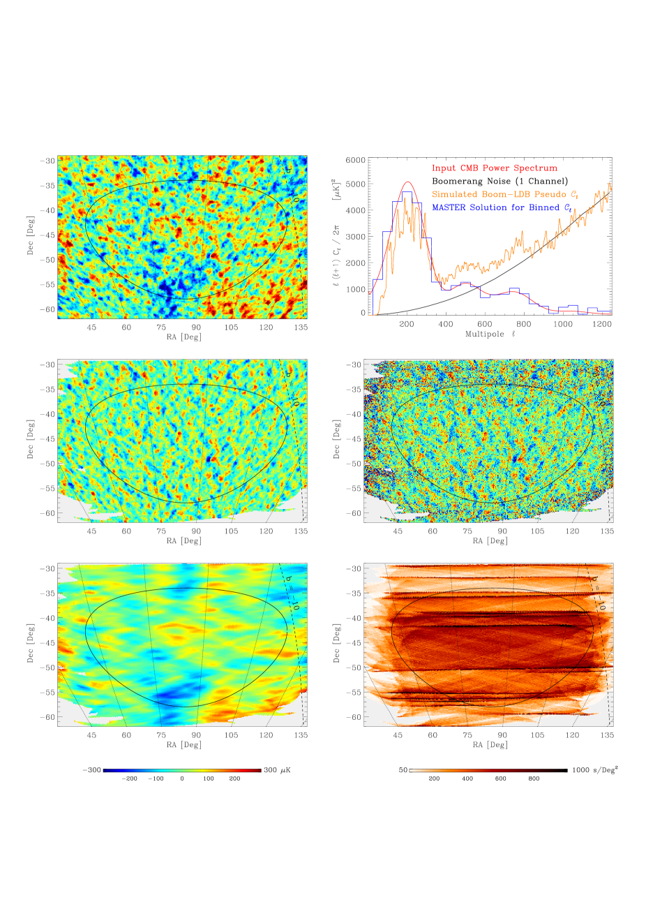
Figure 1: Simulation of the Boom-LDB experiment and application of MASTER to extract the CMB angular power spectrum. The oval contour on the maps shows the ellipse (distorted by projection) within which the power spectrum is estimated (${f_{\rm sky}}=1.8\%$ of the sky). Top left panel: A random realisation of the CMB sky from the theoretical model described by the power spectrum shown in the top right panel (red line). Middle left panel: A noiseless map of the same region of the sky made from the TOD with actual Boom-LDB pointing and processed with the 100 mHz high-pass filter (see text). Bottom left panel: the difference between the two CMB sky maps shown above, which shows the component of the sky signal lost due to the combination of Boomerang scanning and data processing. Middle right panel: A simulation of the same Boomerang CMB sky map with the instrumental noise included. Bottom right panel: Integration time per pixel for the actual scanning of the Boom-LDB  channel B150A; the average integration time is about 500s/Deg². Top right panel: The input power spectrum smoothed by the beam and pixel window function (red line); The average angular power spectrum of the instrumental noise (black line); The pseudo $C_{\ell}$-s directly measured on the sky map shown in the middle right panel and divided by ${f_{\rm sky}}$ (orange line); The binned MASTER estimate of the full sky power spectrum after removal of noise contribution and correction of the effect of the high pass filtering and mode-mode coupling (blue histogram).

A sky temperature fluctuation map $\Delta T({\bf{n}})$ on which a window $W({\bf{n}})$ is applied can be decomposed in spherical harmonics coefficients

$$\tilde{a}_{\ell m} = \int d{\bf{n}}\Delta T({\bf{n}})W({\bf{n}})Y^{*}_{\ell m}({\bf{n}})$$ (11)

$$\approx \Omega_{p}\sum_{p}\Delta T(p)W(p)Y^{*}_{\ell m}(p),$$ (12)

where the integral over the sky is approximated by a discrete sum over the pixels that make the map, with an individual surface area $\Omega_{p}$.

The pseudo power spectrum $\widetilde{C}$ can be defined as

$$\widetilde{C}_{\ell}=\frac{1}{2\ell+1}\sum_{m=-\ell}^{\ell}\left|{\tilde{a}_{\ell m}}\right|^{2}.$$ (13)

The computation of Eq. (12) for each $(\ell,m)$ up to $\ell={\ell_{\rm max}}$ performed on an arbitrary pixelisation of the sphere would scale as ${N_{\rm pix}}{\ell_{\rm max}}^{2}$. However, if one uses an adequate lay out of the pixels to exploit the symmetries of Spherical Harmonics, such as for example the ECP (Muciaccia et al. 1997), HEALPix (Górski et al. 1998), or Igloo (Crittenden and Turok 1998) this computation actually scales like ${N_{\rm pix}}^{1/2}{\ell_{\rm max}}^{2}$. In our implementation of the MASTER method, after application of the window function on the map, the program anafast from the package HEALPix was used to compute the pseudo power spectrum.

Wandelt, Hivon & Górski (2000) showed that the marginalised likelihood $P(\widetilde{C}_{\ell}|{C^{\rm th}},N)$ of the pseudo $\widetilde{C}_{\ell}$ for a given underlying theory ${C^{\rm th}}$ and a given noise covariance $N$ can be computed analytically in ${\mathcal{O}}({N_{\rm pix}}^{1/2}{\ell_{\rm max}}^{2})$ operations, under conditions of axisymmetric sky window function and (non necessarily uniform) white noise. Under these assumptions $P(\widetilde{C}_{\ell}|{C^{\rm th}})$ can be used to perform a maximum likelihood fit of the cosmological parameters to the observed data set. Hansen et al (2001) extend this approach by using the full pseudo $\widetilde{C}_{\ell}$ covariance matrix. We will now build, starting from the measured $\widetilde{C}_{\ell}$, and under more general conditions on the noise properties and shape of the observing window, a new estimator of the full sky power spectrum that can be compared directly to ${C^{\rm th}}$.

3 From Pseudo Power Spectrum to Full Sky Power Spectrum Estimator

The pseudo power spectrum $\widetilde{C}_{\ell}$ rendered by the direct spherical harmonics transform of a partial sky map, Eq. (13), is clearly different from the full sky angular spectrum $C_{\ell}$, but their ensemble averages can be related by

$$\langle{\widetilde{C}}_{\ell}\rangle=\sum_{\ell^{\prime}}M_{\ell\ell^{\prime}}\langle C_{\ell^{\prime}}\rangle,$$ (14)

where $M_{\ell\ell^{\prime}}$ describes the mode-mode coupling resulting from the cut sky. As described in the appendix, this kernel depends only on the geometry of the cut sky and can be expressed simply in terms of the power spectrum ${\mathcal{W}}_{\ell}$ of the spatial window applied to the survey (see Eq. (A43) and Eq. (A14) for the spherical and planar geometry, respectively).

The effect of the instrumental beam, experimental noise, and filtering of the TOD stream can be included as follows

$$\langle{\widetilde{C}}_{\ell}\rangle=\sum_{\ell^{\prime}}M_{\ell\ell^{\prime}}F_{\ell^{\prime}}B^{2}_{\ell^{\prime}}\langle C_{\ell^{\prime}}\rangle+\langle\widetilde{N}_{\ell}\rangle,$$ (15)

where $B_{\ell}$ is a window function describing the combined smoothing effects of the beam and finite pixel size, $\langle\widetilde{N}_{\ell}\rangle$ is the average noise power spectrum, and $F_{\ell}$ is a transfer function which models the effect of the filtering applied to the data stream or to the maps. The determination of each of these terms will be described below.

It is often assumed that the $\chi^{2}_{\nu=2\ell+1}$ distribution of $C_{\ell}$-s on the full sky can be generalised to cut sky observations by scaling $\nu$ to the number of dof effectively available. Given the large value of $\nu$ the central limit theorem is also invoked to further simplify this to a Gaussian of the same mean and variance. From these successive (and excessive) simplifications we will only retain, as a rule of thumb, that the rms of $C_{\ell}$ averaged over a range $\Delta\ell$ is approximately

$$\Delta C_{\ell}\approx\left(C_{\ell}+\frac{N(\ell)}{B^{2}(\ell)}\right)\sqrt{\frac{2}{\nu_{\ell}}},$$ (16)

with

$$\nu_{\ell}=(2\ell+1)\Delta\ell{f_{\rm sky}}\frac{w_{2}^{2}}{w_{4}},$$ (17)

where the factor $w_{2}^{2}/w_{4}$ accounts for the loss of modes induced by the pixel weighting. We will show in section 4 how this compares to the results of Monte Carlo simulations.

3.1 Mode-mode Coupling Kernel

The resolution in $\ell$ of the measured power spectrum is ultimately determined by the extent of the oberved area of the sky, its geometrical shape, and the pixel weighting $W({\bf{n}})$ applied to the survey (see Hobson & Magueijo 1996, and Tegmark 1996). Although we only tested numerically the method on a circular or elliptically shaped window, nothing prevents the use of a more complex window, specially for a pixel starved experiment with a nonconvex survey area, for which a well designed apodisation could help improving the achievable spectral resolution. We will show in section (4) how the choice of window changes the estimated $C_{\ell}$ spectrum.

3.2 TOD Filter Transfer Function

The transfer function $F_{\ell}$ introduced in Eq. (15) describes the effect of any filtering applied to the TOD stream or to the map on the angular power spectrum. A specific example of the latter is the removal of parallel stripes extending along a direction different from the scanning direction observed in some channels of the Boom-LDB  data (Netterfield et al. 2001, Contaldi et al. 2001). The filtering of the TOD has broader applications, however, and can take the form of a high pass filtering that serves several purposes, as follows:

• reduce the contribution of the low frequency noise (1/f noise) to the map, specially if the scanning strategy and/or the map making technique used do not optimize the removal of these modes,

• reduce the scan or spin synchronous noise, which may appear at the scan frequency and its harmonics,

• remove from the signal the contribution from the large scale anisotropies, which are poorly constrained on an incomplete sky survey, and are likely to contaminate the estimated power spectrum at all the smaller scales.

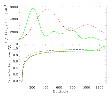
Figure 2: Transfer function of the measured angular power spectrum corresponding to the sharp high pass filtering at 100 mHz of the Boom-LDB TOD is shown here derived for for two different input CMB anisotropy power spectra. The upper panel shows the two input spectra corresponding to a flat Universe (green solid line), and an open Universe (red dashed line). The bottom panel shows the respective transfer functions, which differ by less than 1% up to $\ell=1000$. The black dotted line shows the analytical prediction for a toy model of parallel scans (Eqs. B11, B12).

It should be noted that the validity of Eq. (14) for any sky window relies on the fact that the statistical properties of the full sky temperature fluctuations are isotropic, as implied by Eq. (7). This assumption is broken by the high pass filtering of the data stream which creates a preferred direction on the sky. Therefore the introduction of the single scalar function $F_{\ell}$ in Eq. (15) should be seen as a simplifying ansatz for a more complex reality. We can numerically test the validity of this ansatz by showing for instance that $F_{\ell}$ depends weakly on the choice of the underlying power spectrum.

Given an input CMB power spectrum ${C_{\ell}^{\rm th}}$, a number, ${{N_{\rm MC}^{\rm(s)}}}$, of noise-free full sky realizations of this spectrum can be simulated (using for example the program synfast from HEALPix). These maps are then “observed” using the actual scanning strategy, the resulting model TODs projected back on the sky using Eq. (3), and their individual power spectra $\widetilde{C}_{\ell}$ are extracted using Eqs. (12) and (13).

Equation (15) can then be applied to the average $\langle{\widetilde{C}}_{\ell}\rangle_{MC}$ of these measurements to determine the transfer function. In order to avoid inverting the kernel $M_{\ell\ell^{\prime}}$ this system can be solved iteratively. In the case of a scanning experiment, such as Boomerang, Appendix B shows how a model of parallel scan can render a first order solution ${F^{(0)}}$. In the more general cases, a starting solution could be $F^{(0)}_{\ell}=\langle{\widetilde{C}_{\ell}}\rangle_{MC}/({f_{\rm sky}}w_{2}B^{2}_{\ell}{C_{\ell}^{\rm th}})$. If $\langle{\widetilde{C}}_{\ell}\rangle_{MC}$ is replaced by its running average $S(\langle{\widetilde{C}}_{\ell}\rangle_{MC})$ (typically computed over $\Delta\ell=50$ points) it appears that one iteration is sufficient to obtain a stable estimate of the transfer function

$$F_{\ell} = F^{(0)}_{\ell}$$

$$+ \frac{S\left(\langle{\widetilde{C}}_{\ell}\rangle_{MC}\right)-\sum_{\ell^{\prime}}M_{\ell\ell^{\prime}}F^{(0)}_{\ell^{\prime}}B^{2}_{\ell^{\prime}}\langle C_{\ell^{\prime}}\rangle}{B^{2}_{\ell}\langle C_{\ell}\rangle{f_{\rm sky}}w_{2}}.$$

We used Eq. (3.2) to compute the transfer function in Monte Carlo simulations of Boom-LDB  observations on an elliptically shaped region which comprises 1.8% of the sky (see section 4 for details) for two different input power spectra; the first one corresponding to a flat universe with a first peak at $\ell_{\rm peak}\simeq 220$, and the other one corresponding to an open universe with $\ell_{\rm peak}\simeq 420$. Figure 2 shows that the resulting $F_{\ell}$-s are almost identical, with a discrepancy smaller than 1% in the range $50<\ell<1000$. This justifies the use of the simple ansatz (15) as a model of the effect of the time filtering on the angular power spectrum and demonstrates that the determination of the transfer function can be done nearly independently of any assumptions about the actual CMB power spectrum.

Using approximation (16) one expects that the error $\delta F_{\ell}$ done on the MC estimation of the transfer function decreases as

$$\frac{\delta F_{\ell}}{F_{\ell}}\approx\sqrt{\frac{2}{(2\ell+1)\Delta\ell f_{\rm sky}}}\frac{1}{\sqrt{{N_{\rm MC}^{\rm(s)}}}}.$$ (19)

So if $\Delta\ell f_{\rm sky}\simeq 1$ and $\ell>100$, an estimate of the transfer function better than 1% can be obtained in ${N_{\rm MC}^{\rm(s)}}\mathrel{\mathchoice{\vbox{\offinterlineskip\halign{\hfil$\displaystyle#$\hfil\cr<\cr\vskip 1.5pt\cr\sim\cr}}}{\vbox{\offinterlineskip\halign{\hfil$\textstyle#$\hfil\cr<\cr\vskip 1.0pt\cr\sim\cr}}}{\vbox{\offinterlineskip\halign{\hfil$\scriptstyle#$\hfil\cr<\cr\vskip 0.5pt\cr\sim\cr}}}{\vbox{\offinterlineskip\halign{\hfil$\scriptscriptstyle#$\hfil\cr<\cr\vskip 0.5pt\cr\sim\cr}}}}100$ realisations.

The computation of the transfer function $F_{\ell}$ is required because of the filtered map making technique used (Eq. 3), which alters the signal in low frequency modes. However, even if a more sophisticated map making were used, the map obtained is usually not an unbiased representation of the true sky because of various systematic effects present in the data, and the computation of $F_{\ell}$ is still necessary.

If several detectors with different beams are analysed simultaneously, the realisation of the same sky with a different smearing can be used as an input to the TOD simulation of each detector. In the analysis of the coadded map an effective beam window function $B(\ell)$ can be modeled as the weighted average of all individual beams (see Wu et al. 2001). If the actual effective beam were different from this model the difference would be reflected in the transfer function $F$.

3.3 Noise Power Spectrum

From the point of view of modeling the CMB experiment the simplest form of instrumental noise is the stationary, white, Gaussian process. Reality however is usually not as simple, the actual experimental noise is often non-stationary, “coloured”, sometimes non-Gaussian, and correlated to some internal variables of the instrument, such as its acceleration, the cold plate temperature, the orientation relative to the sun, to the balloon or to the ground. For many of those reasons the noise often can not be efficiently averaged out. However, if these noises can be modeled to a reasonable accuracy, they can be included, at little or no extra cost, in the Monte-Carlo pipeline described here, and their effect on the measured $C_{\ell}$-s can be assessed, and possibly removed.

As mentioned in §2.1 an estimate of the noise time correlation function $N_{tt^{\prime}}$ and its time power spectrum can be extracted from the actual data stream. Using this information a fake Gaussian “noise stream” can be simulated and projected on the sky with the actual scanning strategy using Eq. (3), with the same high pass filtering $f$. The power spectrum $\widetilde{N}(\ell)$ of the resulting noise map is extracted according to Eqs. (12), and (13) and the whole process is reproduced as many times as necessary to obtain a Monte-Carlo estimate of the average noise angular power spectrum, $\langle\widetilde{N}(\ell)\rangle_{MC}$. If several detectors are analysed simulatenously, and their noise is known to be correlated, these correlations can be included in the noise stream simulations.

3.4 Estimated Power Spectrum

In order to reduce the correlations of the $C_{\ell}$-s induced by the cut sky, and also to reduce the errors on the resulting power spectrum estimator, it is convenient to bin the power spectrum in $\ell$. The slowly varying “flattened” spectrum $\mathcal{C}_{\ell}\equiv\ell(\ell+1)C_{\ell}/2\pi$ is a preferable candidate for such binning. For a set of ${n_{\rm bins}}$ bins, indexed by $b$, with respective boundaries $\ell_{\rm low}^{(b)}<\ell_{\rm high}^{(b)}<\ell_{\rm low}^{(b+1)}$, one can define the binning operator $P$ as follows

$$P_{b\ell} = \frac{1}{2\pi}\frac{\ell(\ell+1)}{\ell_{\rm low}^{(b+1)}-\ell_{\rm low}^{(b)}},\quad{\rm if}\quad 2\leq\ell_{\rm low}^{(b)}\leq\ell<\ell_{\rm low}^{(b+1)}$$ (20)

$$= 0,\quad{\rm otherwise}$$

and the binned power spectrum is ${\mathcal{C}}_{b}=P_{b\ell}C_{\ell}$. The reciprocal operator (corresponding to a piece-wise interpolation) then reads

$$Q_{\ell b} = \frac{2\pi}{\ell(\ell+1)},\quad{\rm if}\quad 2\leq\ell_{\rm low}^{(b)}\leq\ell<\ell_{\rm low}^{(b+1)}$$ (21)

$$= 0,\quad{\rm otherwise}.$$

The two operators above are defined for the flat band, disjoint bins. They can be easily modified to account for an $\ell$ dependent weighting within each bin (for example designed to enhance the less noisy multipoles) without changing the rest of the discussion.

Rewriting Eq. (15) as

$$\langle{\widetilde{C}}_{\ell}\rangle=K_{\ell\ell^{\prime}}\langle C_{\ell^{\prime}}\rangle+\langle{\widetilde{N}}_{\ell}\rangle$$ (22)

we then look for a solution to

$$P_{b\ell}K_{\ell\ell^{\prime}}\langle C_{\ell^{\prime}}\rangle=P_{b\ell}\left(\langle{\widetilde{C}}_{\ell}\rangle-\langle{\widetilde{N}}_{\ell}\rangle\right).$$ (23)

This system has ${\ell_{\rm max}}$ unknowns for ${n_{\rm bins}}$ equations. We seek the solution such that $\langle\mathcal{C}_{\ell}\rangle=\ell(\ell+1)\langle C_{\ell}\rangle/2\pi$ is a piece-wise constant. If we replace $\langle C_{\ell}\rangle$ by $Q_{\ell b}P_{bl^{\prime}}\langle C_{\ell^{\prime}}\rangle=Q_{\ell b}\langle\mathcal{C}_{b}\rangle$ then

$$\langle\mathcal{C}_{b}\rangle=K_{bb^{\prime}}^{-1}P_{b^{\prime}\ell}\left(\langle{\widetilde{C}}_{\ell}\rangle-\langle{\widetilde{N}}_{\ell}\rangle\right),$$ (24)

where

$$K_{bb^{\prime}} = P_{b\ell}K_{\ell\ell^{\prime}}Q_{\ell^{\prime}b^{\prime}},$$ (25)

$$= P_{b\ell}M_{\ell\ell^{\prime}}F_{\ell^{\prime}}B^{2}_{\ell^{\prime}}Q_{\ell^{\prime}b^{\prime}}.$$

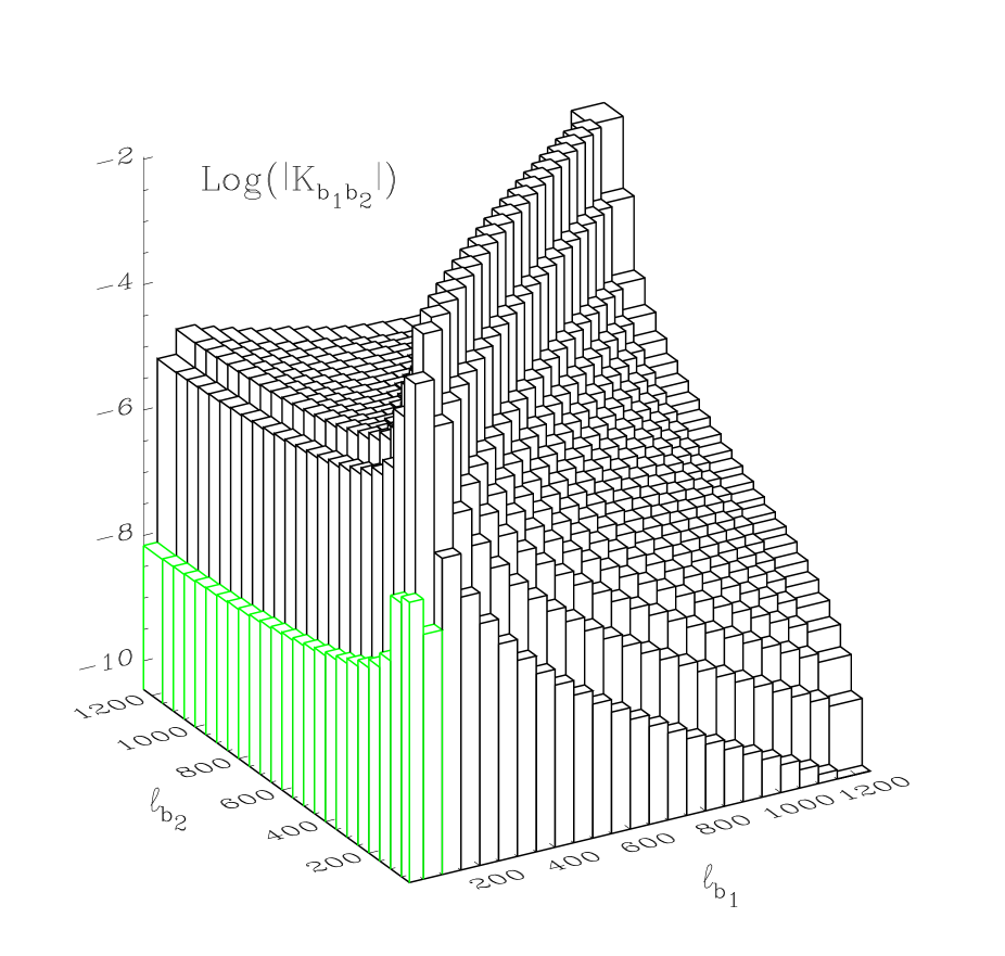
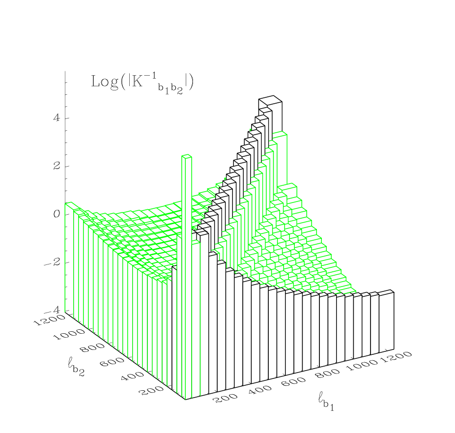
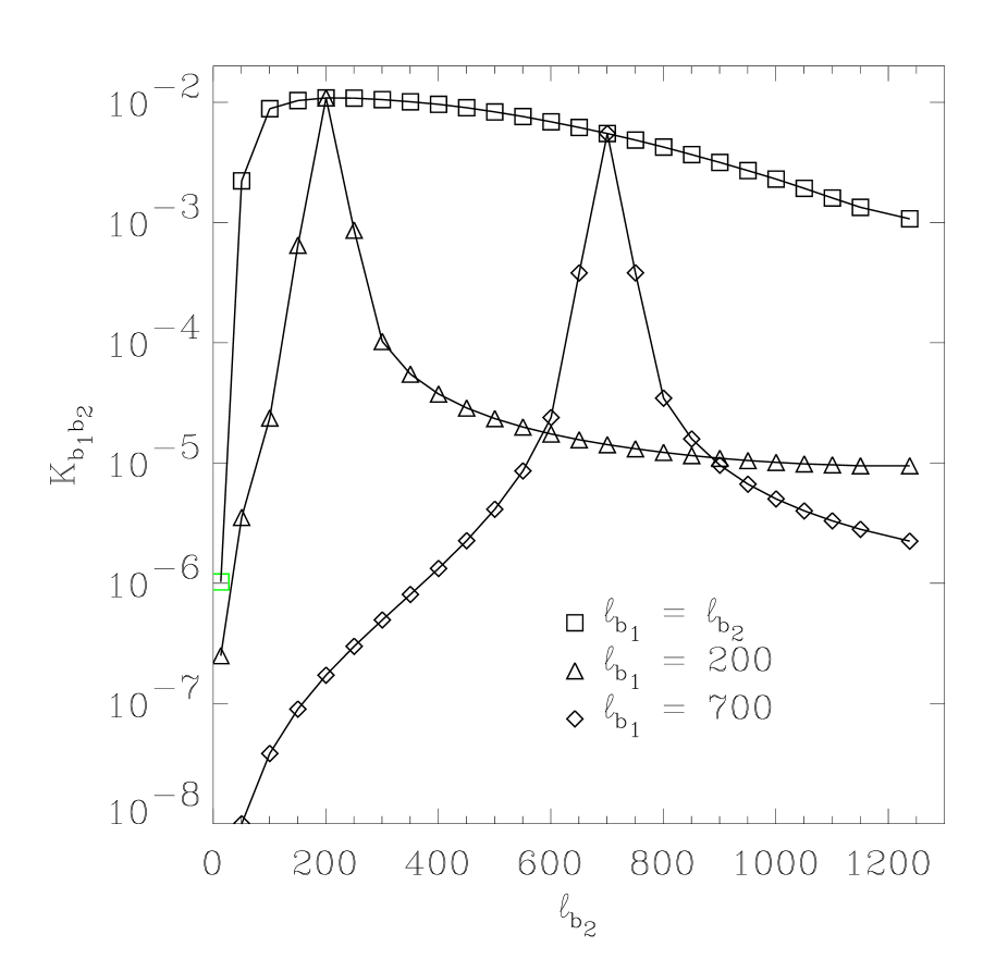
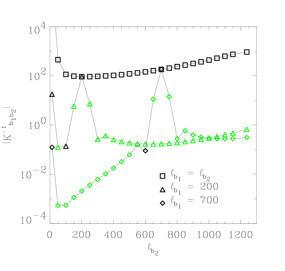
Figure 3: Binned power spectrum coupling kernel $K_{bb^{\prime}}$ and its inverse (absolute values shown, with green color indicating the negative elements) for an elliptically shaped top hat sky window covering 1.8% of the sky. Binwidth is $\Delta\ell=50$, except for the last bin, for which $\Delta\ell=150$. The diagonal elements and the $\ell_{b_{1}}=200,\,{\rm and}\,700$ rows of both matrices are shown in the bottom panels.

An unbiased estimator ${\widehat{\mathcal{C}}}_{b}$ of the whole sky power spectrum is then given by

$$\widehat{\mathcal{C}}_{b}=K_{bb^{\prime}}^{-1}P_{b^{\prime}\ell}\left({\widetilde{C}}_{\ell}-\langle{\widetilde{N}}_{\ell}\rangle_{\rm MC}\right).$$ (26)

An estimator of the noise “on the sky” can also be introduced

$$\widehat{\mathcal{N}}_{b}=K_{bb^{\prime}}^{-1}P_{b^{\prime}\ell}\langle{\widetilde{N}}_{\ell}\rangle_{\rm MC}.$$ (27)

Figure 3 shows the kernel $K_{bb^{\prime}}$ and its inverse for the configuration described in section 4.

It should be noted that the binning of the $\ell$ space is performed at the last stage of the analysis and can be chosen after the MC simulations are done.

3.5 Covariance Matrix of the Estimated Power Spectrum

In order to be able to extract the cosmological parameters from the power spectrum estimated as described above, one needs to know the errors on each ${\mathcal{C}}_{b}$, and the correlations between the bins. This information is contained in the covariance matrix of the estimated power spectrum, which can be estimated as follows. A smooth interpolation of $\widehat{\mathcal{C}}_{b}$ is used as the underlying CMB power spectrum, and a new set of Monte Carlo simulations, including both signal and noise, as well as all the experiment peculiarities, is generated, analysed, and reduced in the same way as the real data. This generates a set of binned power spectrum estimators $\{{\widehat{\mathcal{C}}}_{b}\}$. The elements of the correlation matrix are defined as

$${\bf C}_{bb^{\prime}}=\left\langle\left({\widehat{\mathcal{C}}}_{b}-\langle{\widehat{\mathcal{C}}}_{b}\rangle_{MC}\right)\left({\widehat{\mathcal{C}}}_{b^{\prime}}-\langle{\widehat{\mathcal{C}}}_{b^{\prime}}\rangle_{MC}\right)\right\rangle_{MC}.$$ (28)

The error bars on ${\widehat{\mathcal{C}}}_{b}$ are then given by the square root of the diagonal elements of ${\bf C}$

$$\Delta{\widehat{\mathcal{C}}}_{b}={\bf C}_{bb}^{1/2}.$$ (29)

3.6 The Algorithm

Assuming that for a given CMB experiment the instrumental beam and the time domain power spectrum of the instrumental noise are known, the process of estimation of the full sky power spectrum from the noisy observations of CMB temperature fluctuations can be summarised as follows.

The required tools are :

• a simulation facility for generation of the random realisations of the CMB sky (e.g. synfast from HEALPix),

• a software model of the experiment which simulates observations of the sky using the appropriate scanning strategy (Eq. 1), and generates the model CMB signal TOD streams,

• a noise simulator that can generate random realisations of the noise with an appropriate power spectrum; possible non-gaussian noise features or cross-correlations between detectors should be added at this stage,

• a fast map making facility, which implements Eq. (3), and accounts for any alterations of the observed TOD stream and/or the produced map,

• a software to compute the pseudo power spectrum (Eqs. 12, and 13) from a given apodised cut sky map (e.g. anafast from HEALPix).

After the choice of the sky window apodisation function is made the procedure of estimation of the power spectrum involves the following steps:

1. Eq. (A43) is used to evaluate the $C_{\ell}$ coupling kernel $M_{\ell\ell^{\prime}}$, which accounts for the effects of limited sky coverage and apodisation;

2. a number ${N_{\rm MC}^{\rm(s)}}$ of noise free Monte Carlo simulations of the observed TOD (produced with (a) and (b1), projected on the sky with (b3), and analysed with (c)) are used to estimate the transfer function $F_{\ell}$ of any filtering that is applied to the actual TOD stream;

3. a number ${N_{\rm MC}^{\rm(n)}}$ of pure noise Monte Carlo simulations of the TODs (made with (b1) and (b2), and then projected and analysed with (b3) and (c)) are used to estimate the angular power spectrum $\langle\widetilde{N}\rangle_{MC}$ of the noise projected on the sky;

4. the experimental TOD is coverted into a map using (b3) and its pseudo power spectrum ${\widetilde{C}}_{\ell}$ is obtained with (c);

5. next a set of $\ell$-bins is defined, and an estimate of the underlying full sky binned power spectrum is computed using Eq. (26); according to Eq. (24) this is an unbiased estimator — $\langle{\widehat{\mathcal{C}}_{b}}\rangle=\langle{{\mathcal{C}}_{b}}\rangle$; this will be demonstrated in section 4 with simulated Boomerang observations in which the input spectrum is known;

6. the covariance matrix ${\bf C}_{bb^{\prime}}$ (Eq. 28) is computed from ${N_{\rm MC}^{\rm(s+n)}}$ simulations of the whole experiment, and the error bars on the binned power spectrum are obtained from its diagonal elements (Eq.29).

We assumed the physical beam to be close enough to axisymmetric so that its smoothing effect on the temperature map is independent of the payload attitude along the line of sight. It it were not the case, a direct integration of the temperature over the beam would have to be performed for each time sample in Eq. (1). This operation could be very intensive for extremely structured beams, unless some symmetries in the scanning strategy, such as the one expected for satellite missions, allow for a fast convolution implementation (Wandelt & Górski 2000, Challinor et al, 2000)

On the other hand, the effect of a pointing inacurracy, whether it is axisymmetric or not, can easily be included in the method by modifying Eq. (1) accordingly.

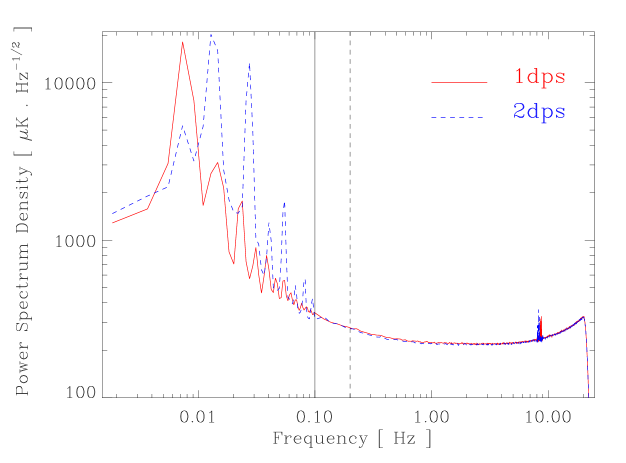
Figure 4: Spectral densities of the noise measured for one of the Boom-LDB channels is shown for the two scanning speeds (1 and 2 degrees per second) of the actual CMB observations. These spectra were used to generate the simulated observations. A sharp high-pass filter was applied to the measured and simulated TODs at 100 and 200 mHz, respectively.

3.7 Computational Scaling

The algorithm is maximally parallelisable as each Monte Carlo cycle of the algorithm can be performed on a separate CPU. Therefore the total time required for completion of the estimation of the power spectrum from the single detector CMB observations, with ${{N_{\rm MC}}}={{N_{\rm MC}^{\rm(s)}}}+{{N_{\rm MC}^{\rm(n)}}}+{{N_{\rm MC}^{\rm(s+n)}}}$ cycles run on ${n_{\rm CPU}}$ processors, is given by

$$T_{\rm~{}total}=\frac{{N_{\rm MC}}}{n_{\rm CPU}}T_{\rm~{}MC~{}cycle}$$ (30)

with $T_{\rm~{}MC~{}cycle}=T_{(a)}+T_{(b)}+T_{(c)}$, where (a),(b), and (c) refer to the CPU time consumption by the simulation tools described in section 3.6 (CMB map synthesis, observation simulation and map making, and map analysis, respectively). In the case of joint multi-detector analysis the stage (b) has to be repeated for each detector, whereas the stage (a) only has to be repeated for each different beam. In our own implementation (see section 4 for detailed specifications) the MASTER method is executed on personal computers (PCs) equipped with 850 MHz AMD Athlon CPUs, the following performance is achieved (on each processor):

$$T_{(a)}=T_{(c)}\simeq 300\ {\rm s}\ \left(\frac{{N_{\rm pix}}}{3\ 10^{6}}\right)^{1/2}\left(\frac{{\ell_{\rm max}}}{1300}\right)^{2},$$ (31)

and

$$T_{(b)}\simeq 300\ {\rm s}\ \left(\frac{{N_{\tau}}}{5\ 10^{7}}\right)\left(\frac{\log{N_{\rm FFT}}}{\log(5\ 10^{5})}\right),$$ (32)

where ${N_{\rm pix}}$ is the number of pixels over the whole sky at the chosen map resolution (not in the cut sky map), ${N_{\tau}}$ is the number of time samples in the TOD set used, and ${N_{\rm FFT}}$ is the typical number of time samples on which the required FFTs are computed. This leads to an overall CPU time requirement of

$$T_{\rm total}=0.5\ {\rm day}\ \left(\frac{{N_{\rm MC}}}{300}\right)\left(\frac{8}{n_{\rm CPU}}\right).$$ (33)

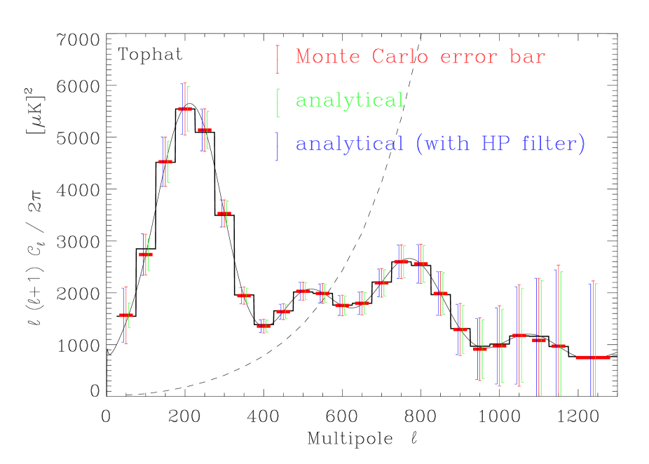
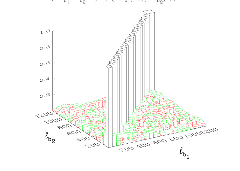
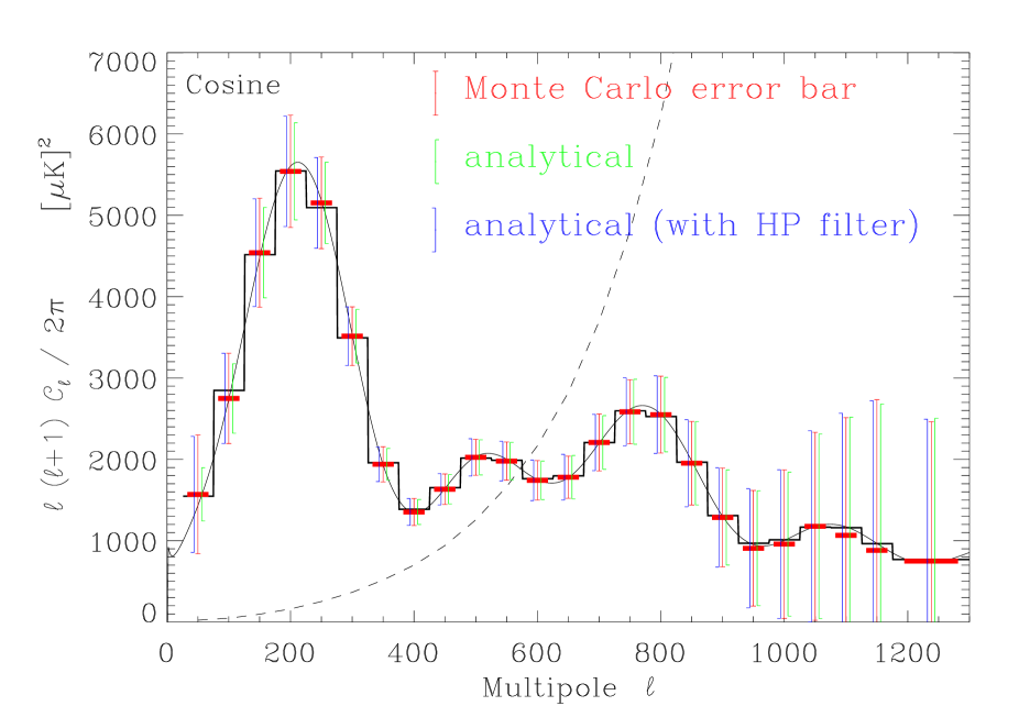
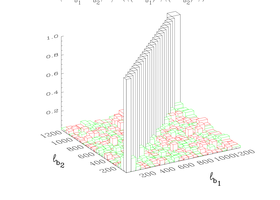
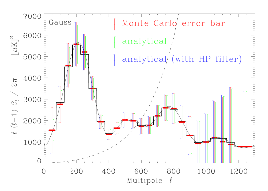
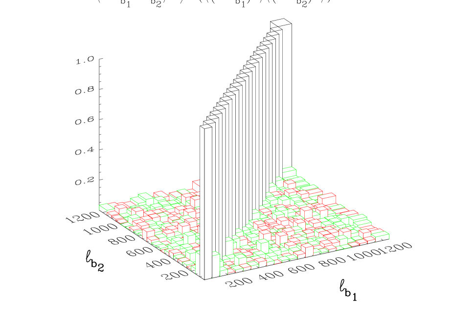
Figure 5: Results of the test of accuracy of our method of estimation of the CMB power spectrum are shown in application to the simulated Boom-LDB  data (with known input power spectrum) with three different sky window apodisations (top hat, cosine and Gaussian from top to bottom panels). We used an ensemble of 1352 Monte Carlo simulations. Left panels: The input power spectrum is shown as a solid black line, and the black histogram shows its bin-averaged values. The dashed lines show the average spectra of the simulated noise. The red histogram shows our MASTER ensemble mean values of the estimated bin-averaged power spectra, which are in perfect agreement (to an error on the mean) with the input bin-averaged theory. For each spectral bin three error bars are shown, all centered vertically on the mean values of the MASTER estimates, $\langle{\widehat{\mathcal{C}}_{b}}\rangle_{MC}$, and, for clarity, spread around the $\ell$-centers of the bins. The central (red) error bars show the rms values of the MASTER ensemble of estimates, while the right-, and left-shifted (green and blue, respectively) ones show the theoretical error estimates based on Eqs. (35, 36) derived, respectively, without and with an inclusion of the effect of the TOD high-pass filter related spectral transfer function $F_{\ell}$. Right panels: absolute value of normalized binned spectrum correlation matrix ${\bf C}_{bb^{\prime}}/\left({\bf C}_{bb}{\bf C}_{b^{\prime}b^{\prime}}\right)^{1/2}$ (see text). Elements with value in $\left[-0.2,0\right]$ are represented in green, those with value in $\left[0,0.2\right]$ in red and those larger than 0.2 in black.

These timing estimates could be easily improved if some repetitive tasks, such as the translation from sky coordinates to pixel index in (b), or the evaluation of Legendre polynomials in (a) and (c) are precomputed and stored on disc.

NB: The most daunting challenge currently foreseen for CMB anisotropy analysis arises in the process of reduction and interpretation of the data that will be collected during the ESA Planck mission (currently scheduled for launch in 2007). Let us recompute our CPU time requirements to match the parameters which describe some of the Planck High Frequency Instrument specifications. One channel of the HFI with a beam resolution of 5 arcmin should, during one year of observations, return ${{N_{\tau}}}\simeq 5.6\times 10^{9}$ TOD points, which will be used to make a HEALPix full sky map with ${N_{\rm pix}}=5\times 10^{7}$ pixels (of average size of 1.7 arcmin) and which in turn should allow us to estimate the angular power spectrum of the sky signals up to ${\ell_{\rm max}}=3000$. With these specifications, and assuming ${N_{\rm FFT}}\simeq 1.5\times 10^{7}$ (one day), the CPU time required for execution of our current implementation of MASTER becomes

$$T_{\rm~{}total}\simeq 24\ {\rm days}\ \left(\frac{{N_{\rm MC}}}{300}\right)\left(\frac{8}{n_{\rm CPU}}\right)$$ (34)

on currently available PCs. Since dedicated computer servers with 32, or more, processors at least twice as fast as the PCs that we used are already presently available, the quoted total execution time for the MASTER method can be reduced to about 3 days. The extra speed up of the CPUs between now and the launch of Planck (a factor of $\sim 16$ according to Moore’s law) should enable the simultaneous analysis of several Planck channels, with more sophisticated map making and a larger number of MC cycles to improve the power spectrum estimation accuracy, in a total time of a few days. This means that the MASTER approach is fully practical from the point of view of demands related to scientific analysis of the Planck data.

4 MASTER Tests on Simulated Boomerang Observations

4.1 Simulations of CMB Observations During The Long Duration Baloon Flight of Boomerang Experiment

The MASTER method was tested for application to the extraction of the CMB anisotropy power spectrum from the data collected by the Boom-LDB  experiment. These CMB observations comprise a total of about $50\ 10^{6}$ samples which cover about 4.4% of the sky, and were acquired at two different azimuthal sky scan rates of 1 and 2 deg per second (for more details on the Boom-LDB flight see Crill, 2001).

We have modeled these CMB observations of the simulated CMB sky with a scanning pattern identical to that of one of Boom-LDB channels. The instrumental noise generated in this channel was assumed to be Gaussian with a time power spectrum identical to the one measured during the observations. The characteristic features of this noise power spectrum include a $\sim 1/f$ behavior at low frequency, a knee-frequency of about 100mHz, a white noise level of 130 $\mu$K.s^1/2, a series of lines located at the harmonics of the scanning frequency (8 mHz at 1dps, and 16 mHz at 2dps), and some microphonic artifacts at 8 Hz (see fig 4). Angular resolution of this channel was FWHM $\approx 10$ arcmin, and we used the actual measured beam profile in the calculations.

The high-pass filtering applied during the process of map-making (Eq.3) was a sharp cut off at 100 mHz for the 1dps scan rate, and 200 mHz for the 2dps scan rate.

The sky maps where pixelised using HEALPix with 7 arcmin pixels ($N_{\rm side}=512$). The power spectrum was computed from a subset of the data on an elliptically shaped region of semi-axes $a=20$ and $b=12$ deg, which covers ${f_{\rm sky}}=1.82\%$ of the sky and is centered on the best observed region of the Boom-LDB  flight. As shown in Fig. 1 the sky coverage in this area, and therefore the noise per pixel, is nonuniform. The number of observations per pixel varies between 50 and 1510, with an average of 370, and a standard deviation of 120. The CMB dipole was not included in the sky simulations as the high pass filtering used in map making reduces its rms residual variation in the observed region of the sky to less than 0.3 $\mu$K, negligible compared to the rms amplitude of $\sim 150\,\mu$K of the intrisic small scale CMB fluctuations.

The input CMB anisotropy spectrum used for the CMB sky model was chosen to fit the results of the joint Maxima-Boomerang data analysis (Jaffe et al. 2001): $\Omega=1$, $\Lambda=0.7$, $h=.82$, $\Omega_{b}h^{2}=0.03$ and $n_{s}=0.975$.

The number of MC simulations performed to estimate the noise, the high-pass filter related transfer function, and the $C_{\ell}$ statistics was, respectively, ${N_{\rm MC}^{\rm(n)}}=450$, ${N_{\rm MC}^{\rm(s)}}=250$ and ${N_{\rm MC}^{\rm(s+n)}}=1350$. Such high numbers of MC simulations are not necessary in practice, but were executed here to test accurately for possible biases, and to measure to a good precision the statistical distribution of the $C_{\ell}$ estimates. Three different apodisations of the analysed sky region, described in Table 1, were used for power spectrum estimation.

Apodisation	$W(r\leq\rho(\phi))$	$w_{2}^{2}/w_{4}$
Top-hat	$1$	$1$
Cosine	$\cos\left(\frac{\pi\ r}{2\ \rho(\phi)}\right)$	$0.514$
Gaussian	$\exp\left({-\frac{1}{2}\left(\frac{3r}{\rho(\phi)}\right)^{2}}\right)$	$0.223$

Table 1: Apodisation applied to the elliptically shaped region of the sky used for extraction of the CMB anisotropy power spectrum. $\rho(\phi)=a/\sqrt{1+(a^{2}/b^{2}-1)\sin^{2}\phi}$ is the radius of the ellipse in a direction $\phi$, and $w_{i}=\int d{\bf{n}}W({\bf{n}})^{i}/4\pi{f_{\rm sky}}$

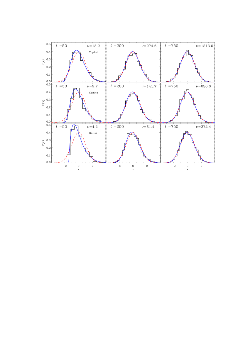
Figure 6: Statistical distribution of the MASTER estimates of the binned full sky CMB anisotropy power spectrum are shown for the bins centered at $l=50,\ 200,\ {\rm and}\ 750$. The results of application of three different sky window apodisations, the Tophat, Cosine, and Gaussian, are shown in top to bottom panels, respectively. The abscissa shows the values of the binned spectrum estimates, ${\widehat{\mathcal{C}}}_{b}$, centered and normalised with the theoretical values used in the MASTER simulations: $x=({\widehat{\mathcal{C}}}_{b}-{\mathcal{C}}_{b}^{\rm th})/\Delta{\widehat{\mathcal{C}}}_{b}$ (see Eq. 36). The histogram shows the distribution derived from the MASTER simulations, the (blue) solid line is derived from the $\chi^{2}_{\nu}$ model where $\nu$ is given by Eq. (35), and the (red) dashed line a Gaussian of same mean and variance.

4.2 Statistics of Binned Spectrum Estimates

Figure 5 shows the Monte Carlo averages and errors on the estimated ${\widehat{\mathcal{C}}}_{b}$-s, computed with the binwidth $\Delta l=50$ for the three used sky window apodisations.

Clearly, the average recovered power spectrum is very close to the input one both at small $\ell$-s, where the signal is dominant, and at large $\ell$-s, where the signal to noise ratio is very low. This demonstrates that the estimator (26) is not biased. The error bars obtained from the Monte Carlo simulations (Eq. 29) can be compared to the “naive” ones (Eq. 16) corrected for the transfer function $F_{\ell}$. This effect decreases the effective number of modes at each $\ell$ to

$$\nu_{b}^{f}=(2\ell_{b}+1)\,\Delta\ell\,{f_{\rm sky}}\,\frac{w_{2}^{2}}{w_{4}}F_{\ell_{b}},$$ (35)

which renders the new analytical error estimate

$$\Delta{\widehat{\mathcal{C}}}_{b}=\left({{\mathcal{C}}}_{b}^{\rm th}+{\widehat{\mathcal{N}}}_{b}\right)\sqrt{\frac{2}{\nu_{b}^{f}}}.$$ (36)

Figure 5 shows that the MC error bars are almost identical to these analytical estimates. Figure 5 also shows the spectrum estimate bin-bin correlation matrix, renormalised such that the diagonal is unity. This matrix is diagonally dominated and except for the first few bins, the off-diagonal elements are at most 10% as large as the diagonal elements.

The distribution of the MASTER ${\widehat{\mathcal{C}}}_{b}$ estimators measured in an $\ell$-bin $b$ defines the likelihood $P({\widehat{\mathcal{C}}}_{b}|{\mathcal{C}}^{\rm th})$ of measuring ${\widehat{\mathcal{C}}}_{b}$ given the input power spectrum ${\mathcal{C}}^{\rm th}$ (after likelihood marginalisation over all the other bins). This distribution was estimated from 1352 Monte Carlo simulations, and is illustrated in figure 6. The histograms show the simulated distribution together with the scaled $\chi^{2}_{\nu}$ model, where $\nu$ (given by Eq. 35) is indicated on each panel, and a Gaussian distribution with the same mean and variance, which becomes undistinguishable from the $\chi^{2}$ curve for large $\nu$. At all $\ell$-s, and specially for small values of $\nu$, the $\chi^{2}$ model, which has no free parameters, gives a much better description of the actual distribution than the Gaussian.

To estimate the cosmological parameters one seeks a theoretical model ${C_{\ell}^{\rm th}}$ defined by these parameters, for which the likelihood $P({\mathcal{C}}^{\rm th}|{\widehat{\mathcal{C}}}_{b})$ constructed for a given data set is maximised. Using the Bayes theorem, this can be rewritten as

$$P({\mathcal{C}}^{\rm th}|{\widehat{\mathcal{C}}}_{b})\propto P({\widehat{\mathcal{C}}}_{b}|{\mathcal{C}}^{\rm th})P({\mathcal{C}}^{\rm th}),$$ (37)

where $P({\mathcal{C}}^{\rm th})$ is the prior on the cosmological parameters. The term $P({\widehat{\mathcal{C}}}_{b}|{\mathcal{C}}^{\rm th})$ is often assumed to be a Gaussian function of the data ${\widehat{\mathcal{C}}}_{b}$, whereas its dependence on the theory ${\mathcal{C}}^{\rm th}$ can be approximated by an offset-lognormal function (Bond, Jaffe & Knox 2000). We see however from Fig. 6 that for experiments with small sky coverage, the likelihood $P({\widehat{\mathcal{C}}}_{b}|{\mathcal{C}}^{\rm th})$ has to be described at small $\ell$-s as $\chi^{2}$ function of ${\widehat{\mathcal{C}}}_{b}$ to avoid biasing the power spectrum estimation and the cosmological parameters extracted from it.

4.3 Monte Carlo Convergence of the Power Spectrum Estimator

We checked, in the Monte Carlo simulations described above, that the estimators for the transfer function, the noise power spectrum (on the sky), and the accuracy of the error on ${\widehat{\mathcal{C}}}_{b}$ converge with the number of MC cycles, respectively, as follows

$$\frac{\delta F_{\ell}}{F_{\ell}}\sim a\;10^{-2}\sqrt{\frac{100}{{N_{\rm MC}^{\rm(s)}}}}\sqrt{\frac{400}{\ell}}$$ (38)

with $a$ between 0.6 and 0.9, depending on the sky window used;

$$\frac{\delta{\widehat{\mathcal{N}}}_{b}}{{\widehat{\mathcal{N}}}_{b}}\sim 0.6\ 10^{-2}\sqrt{\frac{100}{{N_{\rm MC}^{\rm(n)}}}}\sqrt{\frac{400}{\ell_{b}}}\sqrt{\frac{50}{\Delta\ell}},$$ (39)

and

$$\frac{\delta(\Delta{\widehat{\mathcal{C}}}_{b})}{\Delta{\widehat{\mathcal{C}}}_{b}}\sim 0.1\sqrt{\frac{100}{{N_{\rm MC}^{\rm(s+n)}}}}.$$ (40)

The contribution of the MC based estimation of $F$ and ${\widehat{\mathcal{N}}}$ to the error on the recovered power spectrum is

$$\frac{\delta{\widehat{\mathcal{C}}}_{b}}{{\widehat{\mathcal{C}}}_{b}}=\frac{\delta F_{\ell}}{F_{\ell}}+\frac{\delta{\widehat{\mathcal{N}}}_{b}}{{\widehat{\mathcal{N}}}_{b}}\frac{\widehat{\mathcal{N}}_{b}}{{\widehat{\mathcal{C}}}_{b}}$$ (41)

and can be as low as a few percent for ${N_{\rm MC}^{\rm(s)}}\sim{N_{\rm MC}^{\rm(n)}}\sim 100$ in the signal dominated regime where ${\widehat{\mathcal{N}}}_{b}\ll{\widehat{\mathcal{C}}}_{b}$. In the noise dominated regime, the ratio of the method induced uncertainty $\delta{\widehat{\mathcal{C}}}_{b}$ to the statistical error $\Delta{\widehat{\mathcal{C}}}_{b}$ is

$$\frac{\delta{\widehat{\mathcal{C}}}_{b}}{\Delta{\widehat{\mathcal{C}}}_{b}}\simeq 0.1\sqrt{\frac{100}{{N_{\rm MC}^{\rm(n)}}}},$$ (42)

can be brought below $10\%$ in about 100 Monte Carlo simulations and analysis of pure noise TOD streams. Similarly, from Eq. (40), estimates of the indidual statistical errors of each binned $\Delta{\widehat{\mathcal{C}}}_{b}$ better than 10% can be obtained with a few hundred MC cycles. We have seen however in section 4.2 that it is possible to predict analytically these errors with great accuracy.

5 Conclusions

We have introduced a MASTER method for rapid estimation of the angular power spectrum of the CMB anisotropy from the modern CMB data sets. The method is based on direct spherical harmonic transform of the observed area of the sky and Monte Carlo simulations of the relevant details of observations and data processing. We demonstrated in an application of the MASTER method to simulated observations of Boom-LDB  that this method renders unbiased estimates of the CMB power spectrum, with error bars very close to optimal. Monte Carlo calibration of the MASTER method requires generation and analysis of $\mathrel{\mathchoice{\vbox{\offinterlineskip\halign{\hfil$\displaystyle#$\hfil\cr<\cr\vskip 1.5pt\cr\sim\cr}}}{\vbox{\offinterlineskip\halign{\hfil$\textstyle#$\hfil\cr<\cr\vskip 1.0pt\cr\sim\cr}}}{\vbox{\offinterlineskip\halign{\hfil$\scriptstyle#$\hfil\cr<\cr\vskip 0.5pt\cr\sim\cr}}}{\vbox{\offinterlineskip\halign{\hfil$\scriptscriptstyle#$\hfil\cr<\cr\vskip 0.5pt\cr\sim\cr}}}}1000$ independent simulated realisations of a given CMB experiment. We demonstrated that CPU time requirements of the MASTER approach permit succesful analysis of the largest CMB data sets that exist at the present time using very modest computer facilities, for example an inexpensive PC farm.

Because of the combination of the unsophisticated map making that we used and the aggressive high pass filtering applied to the Boomerang data stream in our numerical tests of MASTER, the estimated power spectrum at the lowest multipoles ($\ell<100$) has relatively large error bars. We are currently investigating the use of a more sophisticated map making algorithm to try to improve this situation. Ultimately, however, in the large sky coverage experiments, such as MAP or Planck, the power spectrum at low $\ell$-s can be analysed with fully fledged likelihood techniques if a coarsened pixelisation is used.

Possible improvements of the method include the modelisation of specific systematic effects, the use of more sophisticated map making techniques, and the extension to CMB polarisation measurements.

Appendix A Appendix: mode-mode coupling kernel

In this appendix we compute the mode-mode coupling kernel resulting from the cut sky analysis, both in the planar geometry case, where the arithmetics involved may be more familiar and on the sphere.

A.1 Analysis on the plane

A scalar field $\Delta T({\bf{r}})$ defined on the plane (or defined on the sphere and projected on a tangent plane) can be decomposed in Fourier coefficients as follows

$$a({{\bf{k}}})=\int d{\bf{r}}\Delta T({\bf{r}})e^{-2i\pi{\bf{k}}{\bf{r}}},$$ (A1)

and

$$\Delta T({\bf{r}})=\int d{\bf{k}}a({{\bf{k}}})e^{2i\pi{\bf{k}}{\bf{r}}}.$$ (A2)

If $\Delta T$ is the homogeneous, isotropic, Gaussian distributed temperature fluctuation, each $a({\bf{k}})$ is an independent Gaussian random variable with

$$\langle a({{\bf{k}}})\rangle=0,$$ (A3)

and

$$\langle a({{\bf{k}}})a^{*}({{\bf{k}}^{\prime}})\rangle=\delta({\bf{k}}-{\bf{k}}^{\prime})\langle C({\bf{k}})\rangle=\delta({\bf{k}}-{\bf{k}}^{\prime})\langle C(k)\rangle,$$ (A4)

where $\delta$ is the Dirac delta function.

The Fourier coefficients derived on a weighted plane are then

$$\tilde{a}({{\bf{k}}}) = \int d{\bf{r}}\Delta T({\bf{r}})W({\bf{r}})e^{-2i\pi{\bf{k}}{\bf{r}}},$$ (A5)

$$= \int d{\bf{k}}^{\prime}a({{\bf{k}}^{\prime}})K_{{\bf{k}}^{\prime}{\bf{k}}}[W].$$ (A6)

If we write $W({\bf{r}})=\int{d{\bf{k}}}w({{\bf{k}}})e^{2i\pi{\bf{k}}{\bf{r}}}$, the coupling kernel reads

$$K_{{\bf{k}}_{1}{\bf{k}}_{2}} \equiv \int d{\bf{r}}e^{2i\pi{\bf{k}}_{1}{\bf{r}}}W({\bf{r}})e^{-2i\pi{\bf{k}}_{2}{\bf{r}}}$$

$$= \int{\bf{k}}_{3}w({{\bf{k}}_{3}})\int d{\bf{r}}e^{2i\pi{\bf{r}}({\bf{k}}_{1}-{\bf{k}}_{2}+{\bf{k}}_{3})}$$

$$= \int{\bf{k}}_{3}w({{\bf{k}}_{3}})\delta({\bf{k}}_{1}-{\bf{k}}_{2}+{\bf{k}}_{3}).$$ (A8)

If the polar coordinates of the vector ${\bf{k}}_{i}$ are $(k_{i},\theta_{i})$, the following useful property of the Dirac delta function can be demonstrated:

$$\int\int{d\theta_{1}}{d\theta_{2}}\delta({\bf{k}}_{1}+{\bf{k}}_{2}+{\bf{k}}_{3}) = \int{d\theta_{2}}\delta(k_{1}-|{\bf{k}}_{2}+{\bf{k}}_{3}|)/k_{1}$$ (A9)

$$= {2\pi}J(k_{1},k_{2},k_{3}),$$

where the function $J$ is defined as follows

$$J(k_{1},k_{2},k_{3})=\frac{2}{\pi}\left(2k_{1}^{2}k_{2}^{2}+2k_{1}^{2}k_{3}^{2}+2k_{2}^{2}k_{3}^{2}-k_{1}^{4}-k_{2}^{4}-k_{3}^{4}\right)^{-1/2}$$ (A10)

for $|k_{2}-k_{3}|<k_{1}<k_{2}+k_{3}$, and $J=0$ otherwise. It follows that

$$\int d{\bf{k}}_{1}J(k_{1},k_{2},k_{3}) = \pi\int_{(k_{2}-k_{3})^{2}}^{(k_{2}+k_{3})^{2}}d(k_{1}^{2})J(k_{1},k_{2},k_{3})$$ (A11)

$$= 2\int_{-1}^{1}du(1-u^{2})^{-1/2}$$

$$= 2\pi,$$

and $J(k_{1},k_{2},0)=\delta(k_{1}-k_{2})/k_{1}$.

$$\langle\widetilde{C}_{k_{1}}\rangle \equiv \frac{1}{2\pi}\int{d\theta_{1}}\langle\tilde{a}({{\bf{k}}_{1}})\tilde{a}^{*}({{\bf{k}}_{1}})\rangle,$$

$$= \frac{1}{2\pi}\int{d\theta_{1}}\int{d{\bf{k}}_{2}}\int{d{\bf{k}}_{3}}\langle{a}({{\bf{k}}_{2}}){a}^{*}({{\bf{k}}_{3}})\rangle K_{{\bf{k}}_{1}{\bf{k}}_{2}}[W]K^{*}_{{\bf{k}}_{1}{\bf{k}}_{3}}[W]$$

$$= \frac{1}{2\pi}\int{d\theta_{1}}\int{d{\bf{k}}_{2}}\langle C_{k_{2}}\rangle\int{d\theta_{2}}\left|K_{{\bf{k}}_{1}{\bf{k}}_{2}}[W]\right|^{2}$$

$$= 2\pi\int\int k_{2}dk_{2}\,k_{3}dk_{3}\,\langle C_{k_{2}}\rangle\,{\mathcal{W}}(k_{3})\,J(k_{1},k_{2},k_{3}),$$

where ${\mathcal{W}}(k)=\int d\theta w({\bf{k}})w({\bf{k}})^{*}/2\pi$.

This equation can be rewritten as follows

$$\langle\widetilde{C}_{k_{1}}\rangle=\int k_{2}dk_{2}\,M_{k_{1}k_{2}}\langle C_{k_{2}}\rangle,$$ (A13)

where the coupling kernel is given by

$$M_{k_{1}k_{2}}=2\pi\int k_{3}dk_{3}{\mathcal{W}}(k_{3})\,J(k_{1},k_{2},k_{3}).$$ (A14)

If $C(k_{2})=N$ (the white noise spectrum) then

$$\langle\widetilde{C}_{k_{1}}\rangle=2\pi N\int k_{3}dk_{3}{\mathcal{W}}(k_{3}),$$ (A15)

where we used Eq. (A11).

A.2 Analysis on the sphere

A scalar field $\Delta T({\bf{n}})$ defined on the sphere and weighted with an arbitrary window function $W({\bf{n}})$ can be expanded in spherical harmonics as follows

$$\tilde{a}_{\ell m} = \int d{\bf{n}}\Delta T({\bf{n}})W({\bf{n}})Y^{*}_{\ell m}({\bf{n}}),$$ (A16)

$$= \sum_{\ell^{\prime}m^{\prime}}a_{\ell^{\prime}m^{\prime}}\int d{\bf{n}}Y_{\ell^{\prime}m^{\prime}}({\bf{n}})W({\bf{n}})Y^{*}_{\ell m}({\bf{n}}),$$ (A17)

$$= \sum_{\ell^{\prime}m^{\prime}}a_{\ell^{\prime}m^{\prime}}K_{\ell ml^{\prime}m^{\prime}}[W],$$ (A18)

where the kernel $K$ describes the mode-mode coupling resulting from the sky weighting. If $W$ is z-axis azimuthally symmetric, $K_{\ell ml^{\prime}m^{\prime}}=K_{\ell ml^{\prime}m}\delta_{mm^{\prime}}$. See Wandelt, Hivon & Górski (1999) for an analytical calculation of $K_{\ell ml^{\prime}m}$ in the case when $W$ is a tophat window.

Note that $\tilde{a}$ is a linear combination of Gaussian variables and is therefore Gaussian as well, but the $\tilde{a}_{\ell m}$-s are not independent.

If we use the series representaion of the window function, $W({\bf{n}})=\sum_{\ell m}w_{\ell m}Y_{\ell m}({\bf{n}})$, the coupling kernel reads

$$K_{\ell_{1}m_{1}\ell_{2}m_{2}} \equiv \int d{\bf{n}}Y_{\ell_{1}m_{1}}({\bf{n}})W({\bf{n}})Y^{*}_{\ell_{2}m_{2}}({\bf{n}})$$

$$= \sum_{\ell_{3}m_{3}}w_{\ell_{3}m_{3}}\int d{\bf{n}}Y_{\ell_{1}m_{1}}({\bf{n}})Y_{\ell_{3}m_{3}}({\bf{n}})Y^{*}_{\ell_{2}m_{2}}({\bf{n}})$$

$$= \sum_{\ell_{3}m_{3}}w_{\ell_{3}m_{3}}(-1)^{m_{2}}\left[\frac{(2\ell_{1}+1)(2\ell_{2}+1)(2\ell_{3}+1)}{4\pi}\right]^{1/2}$$

$$\quad\quad\times{\left(\begin{array}[]{lcr}\ell_{1}&\ell_{2}&\ell_{3}\\ 0&0&0\end{array}\right)}{\left(\begin{array}[]{lcr}\ell_{1}&\ell_{2}&\ell_{3}\\ m_{1}&-m_{2}&m_{3}\end{array}\right)},$$ (A24)

where we introduced the Wigner 3-$j$ symbol (or Clebsch-Gordan coefficient) ${\left(\begin{array}[]{lcr}\ell_{1}&\ell_{2}&\ell_{3}\\ m_{1}&m_{2}&m_{3}\end{array}\right)}$. Several properties of the 3-$j$ symbol will prove useful. This scalar object describes the coupling of 3 angular momentum vectors (whose squared moduli are $\ell_{i}(\ell_{i}+1)$, and projections on the same axis are $m_{i}$, for $i=1,2,3$) such that the total angular momentum vanishes. ${\left(\begin{array}[]{lcr}\ell_{1}&\ell_{2}&\ell_{3}\\ m_{1}&m_{2}&m_{3}\end{array}\right)}$ is non zero only if the triangle relation

$$|\ell_{1}-\ell_{2}|\leq\ell_{3}\leq\ell_{1}+\ell_{2}$$ (A25)

is satisfied, and

$$m_{1}+m_{2}+m_{3}=0.$$ (A26)

The orthogonality relations of the Wigner symbols read

$$\sum_{\ell_{3}m_{3}}(2\ell_{3}+1){\left(\begin{array}[]{lcr}\ell_{1}&\ell_{2}&\ell_{3}\\ m_{1}&m_{2}&m_{3}\end{array}\right)}{\left(\begin{array}[]{lcr}\ell_{1}&\ell_{2}&\ell_{3}\\ m_{1}^{\prime}&m_{2}^{\prime}&m_{3}\end{array}\right)}=\delta_{m_{1}m_{1}^{\prime}}\delta_{m_{2}m_{2}^{\prime}},$$ (A27)

$$\sum_{m_{1}m_{2}}{\left(\begin{array}[]{lcr}\ell_{1}&\ell_{2}&\ell_{3}\\ m_{1}&m_{2}&m_{3}\end{array}\right)}{\left(\begin{array}[]{lcr}\ell_{1}&\ell_{2}&\ell_{3}^{\prime}\\ m_{1}&m_{2}&m_{3}^{\prime}\end{array}\right)}=\delta_{\ell_{3}\ell_{3}^{\prime}}\delta_{m_{3}m_{3}^{\prime}}\delta(\ell_{1},\ell_{2},\ell_{3})\frac{1}{2\ell_{3}+1},$$ (A28)

where $\delta(\ell_{1},\ell_{2},\ell_{3})=1$ when the triangular relation (A25) is satisfied, and $\delta(\ell_{1},\ell_{2},\ell_{3})=0$ otherwise. Finally, several recursive or closed form relations can be used to compute the $3-j$ symbols. A useful example of the latter is

$${\left(\begin{array}[]{lcr}\ell_{1}&\ell_{2}&\ell_{3}\\ 0&0&0\end{array}\right)}=(-1)^{L/2}\left[\frac{(L-2\ell_{1})!(L-2\ell_{2})!(L-2\ell_{3})!}{(L+1)!}\right]^{1/2}\frac{(L/2)!}{(L/2-\ell_{1})!(L/2-\ell_{2})!(L/2-\ell_{3})!}$$ (A29)

for even $L\equiv\ell_{1}+\ell_{2}+\ell_{3}$ (or equal to 0 for odd $L$), with the asymptotic behaviour for $L\gg 1$

$${\left(\begin{array}[]{lcr}\ell_{1}&\ell_{2}&\ell_{3}\\ 0&0&0\end{array}\right)}^{2}\longrightarrow\frac{2}{\pi}\left(2\ell_{1}^{2}\ell_{2}^{2}+2\ell_{1}^{2}\ell_{3}^{2}+2\ell_{2}^{2}\ell_{3}^{2}-\ell_{1}^{4}-\ell_{2}^{4}-\ell_{3}^{4}\right)^{-1/2}.$$ (A30)

See Edmonds (1957) for further details on Wigner symbols.

The ensemble averaged power spectrum of the random scalar field $\Delta T({\bf{n}})$ on the sphere computed with an arbitrary weighting function $W({\bf{n}})$ can be represented as follows

$$\langle\widetilde{C}_{\ell_{1}}\rangle \equiv \frac{1}{2\ell_{1}+1}\sum_{m_{1}=-\ell_{1}}^{\ell_{1}}\langle\tilde{a}_{\ell_{1}m_{1}}\tilde{a}^{*}_{\ell_{1}m_{1}}\rangle,$$

$$= \frac{1}{2\ell_{1}+1}\sum_{m_{1}=-\ell_{1}}^{\ell_{1}}\sum_{\ell_{2}m_{2}}\sum_{\ell_{3}m_{3}}\langle{a}_{\ell_{2}m_{2}}{a}^{*}_{\ell_{3}m_{3}}\rangle K_{\ell_{1}m_{1}\ell_{2}m_{2}}[W]K^{*}_{\ell_{1}m_{1}\ell_{3}m_{3}}[W]$$

$$= \frac{1}{2\ell_{1}+1}\sum_{m_{1}=-\ell_{1}}^{\ell_{1}}\sum_{\ell_{2}}\langle C_{\ell_{2}}\rangle\sum_{m_{2}=-\ell_{2}}^{\ell_{2}}\left|K_{\ell_{1}m_{1}\ell_{2}m_{2}}[W]\right|^{2}.$$ (A32)

Upon substituting the kernel expansion in terms of Wigner symbols (A24), and reordering the sums, this expression expands to

$$\langle\widetilde{C}_{\ell_{1}}\rangle = \sum_{\ell_{2}}\langle C_{\ell_{2}}\rangle\frac{2\ell_{2}+1}{4\pi}\sum_{\ell_{3}m_{3}}\sum_{\ell_{4}m_{4}}w_{\ell_{3}m_{3}}w^{*}_{\ell_{4}m_{4}}\left((2\ell_{3}+1)(2\ell_{4}+1)\right)^{1/2}$$ (A41)

$$\times{\left(\begin{array}[]{lcr}\ell_{1}&\ell_{2}&\ell_{3}\\ 0&0&0\end{array}\right)}{\left(\begin{array}[]{lcr}\ell_{1}&\ell_{2}&\ell_{4}\\ 0&0&0\end{array}\right)}\sum_{m_{1}m_{2}}{\left(\begin{array}[]{lcr}\ell_{1}&\ell_{2}&\ell_{3}\\ m_{1}&-m_{2}&m_{3}\end{array}\right)}{\left(\begin{array}[]{lcr}\ell_{1}&\ell_{2}&\ell_{4}\\ m_{1}&-m_{2}&m_{4}\end{array}\right)},$$

which can be remarkably simplified with the aid of both the orthogonality relation of the Wigner symbols (A28), and the definition (Eq. 10)of the power spectrum of the window function, ${\mathcal{W}}_{\ell}$. The final expression reads

$$\langle\widetilde{C}_{\ell_{1}}\rangle=\sum_{\ell_{2}}M_{\ell_{1}\ell_{2}}\langle C_{\ell_{2}}\rangle,$$ (A42)

with

$$M_{\ell_{1}\ell_{2}}=\frac{2\ell_{2}+1}{4\pi}\sum_{\ell_{3}}(2\ell_{3}+1){\mathcal{W}}_{\ell_{3}}{\left(\begin{array}[]{lcr}\ell_{1}&\ell_{2}&\ell_{3}\\ 0&0&0\end{array}\right)}^{2}.$$ (A43)

The Wigner symbols can be numerically computed from (A29) or from any equivalent recurrence relations. The equation (A42) expresses the ensemble averaged angular power spectrum measured with an arbitrary window on the sky for the statistically homogeneous and isotropic fluctuations described by an arbitrary ensemble averaged power spectrum over the full sky.

If the input power spectrum is constant, $\langle C_{\ell}\rangle=N$, corresponding to the white noise distributed over the sky, Eq. (A42) can be simplified using the orthogonality relation (A27), and the measured windowed power spectrum is also a constant

$$\langle\widetilde{C}_{\ell}\rangle=N{f_{\rm sky}}w_{2}.$$ (A44)

Appendix B Appendix: transfer function for parallel scans

In the case of Boomerang, or of any scanning survey, a crude estimate of the transfer function corresponding to the high-pass filtering of the TOD, ${F^{(0)}}$ (see the Eq. 3.2), can be obtained by assuming that to first order the scans are parallel and performed at uniform angular speed. In such a case the filtering of the TOD will alter the sky signal structures parallel to scan direction, but leave unchanged the structures orthogonal to the scan direction. If the surveyed area is small enough ($\sim 20$ deg in each direction) the tangent plane approach is sufficient to model the survey. Hence, the map can be decomposed in plane waves

$$\Delta T(x,y)=\int a(k_{x},k_{y})e^{i(k_{x}x+k_{y}y)}$$ (B1)

with $k_{x}=k\cos\theta$ and $k_{y}=k\sin\theta$. The $a({\bf{k}})$ are zero-mean Gaussian variables with a variance

$$\langle a({\bf{k}})a({\bf{k}}^{\prime})^{*}\rangle=\langle P(k)\rangle\delta({\bf{k}}-{\bf{k}}^{\prime}),$$

and the map power spectrum is given by

$$P(k)=\frac{1}{2\pi}\int d\theta\ a({\bf{k}})a({\bf{k}})^{*}.$$

If the scan is performed along the x-axis the map obtained from the filtered TOD is

$$\Delta T_{\rm filt}(x,y)=\int a(k_{x},k_{y})f(k_{x})e^{i(k_{x}x+k_{y}y)},$$

and its power spectrum is

$$P_{\rm filt}(k)=\frac{1}{2\pi}\int d\theta a({\bf{k}})a({\bf{k}})^{*}f(k_{x})^{2}.$$ (B2)

The ensemble averaged filtered power spectrum is

$$\langle P_{\rm filt}(k)\rangle=\langle P(k)\rangle\frac{1}{2\pi}\int d\theta f(k\cos\theta)^{2}.$$ (B3)

Hence, the effect of the TOD filtering on the power spectrum of the map amounts to a simple transfer function given by ($\ell\sim k$)

$${F^{(0)}_{\ell}}=\frac{1}{2\pi}\int d\theta f(k\cos\theta)^{2}.$$ (B4)

If the scan is performed at an azimutal speed $v_{az}$ at an elevation $\theta_{el}$, and the high pass filter applied to the data has a Gaussian form

$$f(\nu)=1-e^{-(\nu/\nu_{c})^{2}/2}$$ (B5)

then

$${F^{(0)}_{\ell}}=2/\pi\ \int_{0}^{\pi/2}d\theta\big{(}1-e^{-(\ell\cos\theta/\ell_{c})^{2}/2}\big{)}^{2},$$ (B6)

where $\ell_{c}=2\pi\nu_{c}/(v_{az}\cos\theta_{el})$. The asymptotic forms of ${F^{(0)}_{\ell}}$ are

$${F^{(0)}_{\ell}} \rightarrow \frac{3}{32}\left(\frac{\ell}{\ell_{c}}\right)^{4},\quad\ell\ll\ell_{c}$$ (B7)

$${F^{(0)}_{\ell}} \rightarrow 1-\frac{\sqrt{8}-1}{\sqrt{\pi}}\frac{\ell_{c}}{\ell},\quad\ell\gg\ell_{c}.$$ (B8)

On the other hand, if the high pass filter is a chosen in the form of a sharp cut at the frequency $\nu_{c}$

$$f(\nu) = 0,\quad\nu<\nu_{c},$$ (B9)

$$f(\nu) = 1,\quad\nu\geq\nu_{c},$$ (B10)

then

$${F^{(0)}_{\ell}} = 0,\quad\ell<\ell_{c},$$ (B11)

$${F^{(0)}_{\ell}} = 1-2/\pi\ \sin^{-1}(\ell_{c}/\ell),\quad\ell\geq\ell_{c}.$$ (B12)

References

deBernardis et al (2000)
deBernardis, P. etal, 2000, Nature 404, 955-959
Bond (1995) Bond, J.R., 1995, Phys. Rev. Lett. 74, 4369
Borrill (1999a)
Borrill, J., 1999a, Proc. of the 3K Cosmology EC-TMR conference,
eds. L. Maiani, F. Melchiorri, N. Vittorio, AIP CP 476, 277 (astro-ph/9903204)
Borrill (1999b)
Borrill, J., 1999b, Proc. of the 5th European SGI/Cray MPP
workshop (astro-ph/9911389)
Challinor et al (2000)
Challinor, A., et al, 2000, astro-ph/0008228
Contaldi et al (2001)
Contaldi et al, 2001, in preparation
Crill (2000)
Crill, 2000, PhD thesis
Crill et al (2001)
Crill, etal, 2001, in preparation
Gorski (1997) Górski, K.M., 1997, Proceedings of
the XXXIst Rencontres de Moriond, ’Microwave Background Anisotropies’ (astro-ph/9701191)
Górski, Hivon & Wandelt (1998)
Górski, K.M., Hivon, E. and Wandelt,
B.D., in ”Analysis Issues for Large CMB Data Sets”, 1998,
eds. A.J. Banday, R.K. Sheth and L. Da Costa, ESO,
PrintPartners Ipskamp, NL, pp. 37-42
(astro-ph /9812350); see also http://www.eso.org/kgorski/healpix/
Halverson (2001)
Halverson, N.W., et al, 2001, astro-ph/0104488
Hanany (2000)
Hanany, S., et al, 2000, ApJ 545, 5
Hansen (2001)
Hansen, F., et al, 2001, in preparation