Multiwavelength Monitoring of the Narrow-Line Seyfert 1 Galaxy Akn 564. I. $ASC\!A$ Observations and the Variability of the X-ray Spectral Components

Abstract

We present a 35 day ASCA observation of the Narrow-Line Seyfert 1 galaxy Akn 564 (catalog MGC +05-53-012), yielding an on-source exposure $\sim$ 1 Ms. The ASCA observation was part of a multiwavelength AGN Watch monitoring campaign. The soft X-ray light curve binned to 256 s reveals trough-to-peak flux variations up to a factor of $\sim 16$ and changes in the fractional amplitude of variability across the observation.

Akn 564 shows small variations in photon index across the observation, with $\Gamma$ in the range 2.45–2.72. The presence of the soft hump component below 1 keV, previously detected in ASCA data, is confirmed. Time-resolved spectroscopy with $\sim$ daily sampling reveals a distinction in the variability of the soft hump and power-law components over a timescale of weeks, with the hump varying by a factor of $\sim 6$ across the 35-day observation compared to a factor 4 in the power-law. This difference in the long-term amplitudes of variation causes changes in the softness ratio across the observation. Flux variations in the power-law component are measured down to a timescale of $\sim 1000$ s and accompanying spectral variability suggests the soft hump is not well-correlated with the power-law on such short timescales. However, some correlated events are observed in the soft hump, UV flux and hard X-ray flux when all are sampled daily. No significant UV to X-ray lags are found, with upper limits $\sim 1$ day.

We detect Fe K$\alpha$ and a blend of Fe K$\beta$ plus Ni K$\alpha$, the line energies indicating an origin in highly ionized gas. Variability measurements constrain the bulk of the Fe K$\alpha$ line to originate within $\sim$ a light week of the nucleus. The large EW of the emission lines may be due to high metallicity in NLS1s, supporting some evolutionary models for AGN.

1 Introduction

Narrow-line Seyfert 1 galaxies (NLS1s) are a subclass of active galactic nuclei (AGN) with relatively narrow permitted optical emission lines (H$\beta$ ${\rm FWHM}$$<$ 2000 ${\rm km\ s}^{-1}$) and a high Fe II/H$\beta$ ratio (Osterbrock & Pogge, 1985; Goodrich, 1989). Historically, the ratio [O III]$\lambda 5007$ $/$ ${\rm H}\beta<3$ has also been used as a defining criteria for the NLS1 objects, although it now appears that this is not a good indicator (Rodriguez-Ardila et al., 2000). Such properties place these galaxies at the lower end of the line-width distribution for the Seyfert 1 population, thus distinguishing them from the bulk of Seyfert 1 galaxies (hereafter “broad-line Seyfert 1s” or BLS1s). Furthermore, Boroson & Green (1992) find NLS1s to exist as one extreme of their primary eigenvector, and conclude that the dominant source of differences in the observed optical properties of low-redshift AGN is a fundamental parameter (which balances Fe II excitation against the illumination of the narrow line region).

In the X-ray regime, NLS1s exhibit rapid and large-amplitude variability (Boller, Brandt, & Fink, 1996, hereafter BBF96). Turner et al. (1999b) showed X-ray variability to be systematically more extreme in NLS1s than in BLS1s despite both having the same luminosity distribution. For a given luminosity, NLS1s show an order of magnitude greater variability, as measured by $\sigma^{2}_{rms}$ (Turner et al., 1999b; Leighly, 1999a). Some NLS1s show X-ray flares up to a factor of 100, on timescales of days (e.g., Forster & Halpern, 1996; Boller, Brandt, & Fabian, 1997), compared to the factors of $\sim$ a few seen in BLS1s. ROSAT (0.1–2.4 keV) observations revealed that the NLS1 soft X-ray continuum slopes are systematically steeper than those of BLS1s (BBF96), the photon index $\Gamma$ (photon flux $P_{\rm E}\propto E^{-\Gamma}$) sometimes exceeding 3. This phenomenon was found to extend to higher energies using ASCA (2–10 keV) observations (Brandt, Mathur, & Elvis, 1997; Turner, George, & Nandra, 1998; Leighly, 1999b; Vaughan et al., 1999b). The very strong anticorrelation between H$\beta$ ${\rm FWHM}$ and both the X-ray spectral slope in Seyferts (BBF96) and in quasars (Laor et al., 1997) and “excess variance” (Turner et al., 1999b) suggests that the remarkable X-ray properties of NLS1s represent an extreme of Seyfert activity, possibly due to an extreme value of a fundamental physical parameter related to the accretion process.

A popular explanation of the differences in X-ray properties across the Seyfert population is that NLS1s have relatively low masses for the central black hole. Smaller black-hole masses naturally explain both the narrowness of the optical emission lines, which are generated in gas that has relatively small Keplerian velocities, and the extreme X-ray variability, since the primary emission would originate in a smaller region around the central engine (e.g., Laor et al., 1997). Given that NLS1s have comparable luminosity to that of the BLS1s, Pounds, Done, & Osborne (1995) suggested that they must be emitting at higher fractions of their Eddington luminosity, hence higher fractional accretion rates ($\dot{m}=\dot{M}/\dot{M}_{\mbox{\scriptsize Edd}}$) are also required.

The closer the luminosity to the Eddington limit (and the lower the black-hole mass), the greater the fraction of the energy emitted by the accretion disk in the soft X-rays (Ross, Fabian, & Mineshige, 1992). Thus NLS1s might be expected to show disk components which peak at higher energies than for BLS1s. Pounds, Done, & Osborne (1995) and Maraschi & Haardt (1997) noted that soft photons from the disk may Compton-cool hard X-rays from the corona, and cause the steep observed photon indices. In the case of a high accretion rate, the surface of the disk is also expected to be highly ionized (Matt, Fabian, & Ross, 1993); evidence of reflection from such a disk (from Fe K$\alpha$) is found in six NLS1s: Comastri et al. (1998), Turner, George, & Nandra (1998) for Ton S180; Vaughan et al. (1999a), Comastri et al. (2001), Turner, George, & Netzer (1999a) for Akn 564; Ballantyne, Iwasawa, & Fabian (2000) for the previous sources plus Mrk 335, NGC 4051, PG 1244+026, and PKS 0558-504. However, lines from ionized Fe are not unique to the NLS1 population, since they sometimes occur in BLS1s as well (e.g., Guainazzi et al., 1998).

Alternative explanations of the difference in observed parameters across the Seyfert population include the possibility that NLS1s have broad-line regions more distant from the nucleus than BLS1s and hence smaller Keplerian line widths (Guilbert, Fabian, & McCray, 1983), or that NLS1s are observed preferentially close to face on. The latter is disfavored by the analysis of Boroson & Green (1992), and the fact that the inner regions of BLS1s also appear to be observed close to face-on (Nandra et al., 1997a). The former possibility can be tested by measuring the size of the broad-line region using reverberation mapping.

Reverberation mapping uses measurements of the correlations between emission-line and continuum flux variations across a broad energy band to determine the size-scales of the emitting regions (Peterson, 1993). Line profiles give the kinematics of the emitting gas, and combining the size and velocity information yields an estimate of the central mass of an AGN (Wandel, Peterson & Malkan, 1999). Results obtained to date have indicated that for NLS1s $M_{\rm BH}\approx 10^{6}M_{\odot}$, as opposed to $M_{\rm BH}\approx 10^{7}-10^{8}\,M_{\odot}$ for BLS1s, while NLS1s and BLS1s appear to have broad-line regions which are comparable in size (Kaspi et al., 2000; Peterson et al., 2000).

Akn 564 (IRAS 22403+2927, MGC +05-53-012) is a bright, nearby NLS1 with $z=0.0247$, (Huchra, Vogeley & Geller, 1999); $V=14.6$ mag, (de Vaucouleurs et al., 1991), and $L_{\mbox{\scriptsize 2--10{} keV}}\approx 2.4\times 10^{43}$ ergs s^-1(from these data); hence an ideal test case for accretion disk models of AGN. ROSAT observations (Brandt et al., 1994) showed a complex soft X-ray spectrum with spectral features around $\sim 1$ keV. However, the PSPC data could not discriminate between absorption or emission as the origin of the complex form of the spectrum. Subsequent ASCA observations ($\sim 50$ ks, Turner, George, & Netzer 1999a; Vaughan et al. 1999a; Leighly 1999b) confirmed the complexity of the soft spectrum and showed a strong iron line at rest energy of about 7 keV, indicative of reflection from highly ionized material. This conclusion was supported by Vaughan et al. (1999b) who detected an edge at 8.5 keV in combined ASCA and RXTE data, attributable to reflection from a strongly irradiated disk. BeppoSAX data (Comastri et al., 2001) are also indicative of reflection from a highly ionized, optically-thick accretion disk.

The most intensive broad-band reverberation mapping program undertaken to date aimed to determine the nature of the relationship between X-ray and UV–optical continuum variations and thus obtain an estimate of the BLR size and virial mass of the central source in the NLS1 galaxy, Akn 564. This campaign was designed to obtain the first estimate for a NLS1 of the size of the region emitting the broad UV lines, and it provided the longest baseline for a quasi-continuous X-ray study of any AGN to date (i.e interrupted only by earth occultation, SAA passage etc). Akn 564 was observed by ASCA on 2000 June 1 to July 6, during a multiwavelength monitoring campaign that included observations from HST between May 9 and July 8 (Collier et al., 2001, Paper II), RXTE between June 1 and July 1 (Pounds et al., 2001; Edelson et al., 2001), and XMM (Brandt et al., 2001) June 17, and from many ground-based observatories as part of the AGN Watch project (Shemmer et al., 2001, Paper III).

In this paper we present the results from the $\sim$ 1 Ms ASCA observation of Akn 564. In § 2 we present the data; in § 3 we discuss the time variability of the source; § 4 we analyze the mean spectrum; in § 5 we discuss time-resolved spectroscopy; § 6 presents an investigation of the RMS spectrum; § 7 looks at the correlations between the X-ray parameters, and with the UV flux at 1365 Å; § 8 presents a summary of our observational results; finally, in § 9 we discuss the X-ray results.

2 Observations and Data Reduction

ASCA is equipped with four focal-plane detectors that are operated simultaneously, namely, two CCDs (the Solid-state Imaging Spectrometers SIS-0 and SIS-1, 0.4–10 keV, Burke et al. 1991) and two gas-scintillation proportional-counters (Gas Imaging Spectrometers GIS-2 and GIS-3, 0.7–10 keV, Ohashi et al. 1996, and references therein). ASCA obtained a total duration of $\sim 2.98$ Ms on Akn 564, starting from JD $=2451697.024$ (for the screened data). The data were reduced using standard techiques as described in Nandra et al. (1997a); in particular, the methods and screening criteria utilized by the Tartarus database (Turner et al., 1999b) were used. Data screening yielded an effective exposure time of $\sim 1.11$ Ms for the SISs and $\sim 1.29$ Ms for the GISs. The mean SIS-0 count rate was 1.894 $\pm 0.001$ cts s^-1 (0.6–10 keV band).

Since launch in 1993, the ASCA SIS detectors have been experiencing a degradation in efficiency at the lower energies, which is probably due to increased dark current levels and decreased charge transfer efficiency (CTE), producing SIS spectra which diverge from each other and from the GIS data. This loss in efficiency is not well understood and therefore not corrected for by any of the software (in particular, CORRECTRDD does not solve the problem), so that the discrepancy between SIS-1 and GISs can be as much as 40% below 0.6 keV for data taken in January 2000. Data from the last phase of ASCA operations, AO-8, revealed that there has been a non-linear evolution of the SIS CTE. The Akn 564 data were first calibrated using linear extrapolations of SIS gain from the last determination of CTE values on 1997 March 11. That calibration produced unacceptably large inconsistencies between the SIS and GIS instruments up to a few keV. Thus the previous solution of excluding SIS data below 0.6 keV is inadequate. We recalculated the SIS gain using the interim solution released on 2001 February 13 (using CTE file $sisph2pi\_130201.fits$). This interim solution reduced the instrument discrepancies significantly, but still necessitated the exclusion of some sections of the SIS data. For this reason, we proceed as follows. We have modelled the features which appear in both GIS and SIS detectors and ignored residuals which are in one instrument or instrument pair only (and are likely artifacts of calibration problems). We then used our simple parameterization of the data to examine the time-variability of the source spectrum.

The divergence of the SIS detectors at low energies can be partly corrected for in the spectral analysis. One approach (Yaqoob et al., 2000), is to quantify the apparent loss in SIS efficiency as a function of time throughout the mission; an empirical correction can be applied by parameterizing the efficiency loss with a time-dependent absorption (“excess N_H”). The correction for SIS-0 follows the linear relationship, $N_{\rm H}(\mbox{SIS0})=3.635857508\times 10^{-8}\;(\mbox{ {\tt T}}-3.0174828\times 10^{7})\;10^{20}$ cm^-2, where T is the average of start and stop times of the observation, based on seconds since launch. There is no simple analytical relationship that satisfies the SIS-1 excess N_H, but it is usually found that a slightly larger column can be applied to the SIS1 data to bring it into line with SIS0. Naturally, one has to be extremely conservative in interpreting spectral features derived from fits in the lower-energy region, in particular below 1 keV, once this empirical correction has been applied. For our observation, where T $=2.36\times 10^{8}$ s, $N_{\rm H}(\mbox{SIS0})=7.5\times 10^{20}$ cm^-2 and we adopted $N_{\rm H}(\mbox{SIS1})=1.05\times 10^{21}$ cm^-2.

A more conservative approach consists of only considering data above 1 keV for both SIS and GIS, where the disagreement is less dramatic. However, as we are very interested in the variability of the soft hump spectral component, in this paper, we will use the excess $N_{\rm H}{}$ correction for our fitting.

3 The Time Variability

Light curves were extracted using bin sizes of 256 s, and 5760 s in the full-band (0.7-10 keV) for the SIS, a soft-band (0.7–1.3 keV) for the SIS data, and the hard-band (2–10 keV) for both GIS and SIS data. The use of 0.7 keV as a lower limit for the SIS data was due to the high setting for the SIS lower level discriminator towards the end of the observation. In all cases we combined the data from the SIS and GIS detector pairs. The exposure requirements for the combined curves were that the bins be fully exposed in each instrument for the 256 s curves and at least 10 % exposed for the 5760s curves. The observed count rates correspond to a mean 2–10 keV flux of $2\times 10^{-11}$ ${\rm erg\ cm^{-2}\ s^{-1}}$ and 2–10 keV luminosity $2.4\times 10^{43}$ ergs s^-1 (assuming $H_{0}=75$ ${\rm km\ s^{-1}\ Mpc^{-1},}$ $q_{0}=0.5$). This mean flux level is $\sim$ 20 % brighter than that observed during a previous ASCA observation in 1996 December 23 (Turner, George, & Netzer, 1999a). Figure 1 shows the combined 0.7–1.3 keV SIS soft-band and GIS hard-band light curves in 5760 s bins. The background level in the source cell is about 4 % of the source count rate, and not plotted or subtracted. Figure 1 also shows the softness ratio, defined as the ratio between the count rates in the 0.7–1.3 and 2–10 keV bands. The spectrum hardens during the ASCA observation.

The light curves binned to 5760 s show trough-to-peak variations in flux by a factor of $\sim 10$ in the 0.7–1.3 keV band (SIS), $\sim 7$ in the 2–10 keV band (GIS). Examination of light curves binned to 256 s reveals even larger amplitudes due to fast flickering. The maximum amplitude of variability in these (256 s) curves is a factor $\sim 16$ for the SIS data in the 0.7-1.3 keV band and $\sim 14$ for the GIS data in the 2–10 keV band. In their Figure 3, Edelson et al. (2001) show the 0.7–1.3 keV and 2–10 keV light curves, in 256 s bins, for a “flare” at JD $\approx$ 2451710 (centered around 1153 ks after the start of the observation). The SIS and GIS data show rate variations of a factor of 1.4 and 1.8 (respectively) in $\Delta t=1280$ s, corresponding to a variation in luminosity of $\Delta L=1.9\times 10^{43}$ ergs s^-1. The close-up examination of that flare shows that the hard X-ray event is sharper than that in the soft band, and that there is a significant change in softness ratio on a timescale of $\sim 1000$ s (Edelson et al., 2001). Close examination of the light curve reveals other similar examples of rapid changes in spectral shape and also some flares which are not accompanied by a strong spectral change. The behavior of the source is obviously complex with some events characteristically different to others.

Here we concentrate on the search for variations in spectral parameters across the 35 day baseline of the observation to understand the nature of the spectral variability. A more detailed timing analysis is presented in a complementary paper, Edelson et al. (2001).

3.1 Fractional Variability Amplitude

The fractional variability amplitude $F_{\rm var}$ is defined in Edelson et al. (2001), as

$$F_{\rm var}=\sqrt{\frac{S^{2}-\langle\sigma^{2}_{\rm err}\rangle}{\langle X\rangle^{2}}},$$ (1)

where $S^{2}$ is the total variance of the light curve, $\sigma^{2}_{\rm err}$ is the mean error squared, and $\langle X\rangle$ is the mean count rate. The error on $F_{\rm var}$, also from Edelson et al. (2001), is

$$\sigma_{F_{\rm var}}=\frac{1}{F_{\rm var}}\sqrt{\frac{1}{2N}}\frac{S^{2}}{\langle X\rangle^{2}}.$$ (2)

The quantity $F_{\rm var}$ was calculated every $\sim$ day using even sampling and constructing light curves with 256 s bins. We examined the quantity in the soft (0.7–1.3 keV) band and the hard (2–10 keV) band. These bands were chosen to be as widely separated as possible in the energy-bandpass, but having good signal-to-noise in each curve. $F_{\rm var}$ is variable across the observation, but there appears to be no correlation between this quantity and the flux-state of the source, probably due to a random nature of the light curve. $F_{\rm var}$ appears very well correlated between the soft and hard bands. As we will demonstrate in § 4, in the mean spectrum the power-law continuum provides about 75 % of the flux in the 0.7–1.3 keV band. The rapid variations in the power-law component dominate the variability so the two bands have a correlated component of variability, making $F_{\rm var}$ appear similar, to first order, in the soft and hard bands.

$F_{\rm var}$ calculated across the whole dataset is 34.84 % $\pm$ 0.46 for the 0.7–1.3 keV band, and 33.19 % $\pm$ 0.40 for the 2–10 keV band. This quantity measures deviations compared to the mean, integrated over the entire month. The slightly greater $F_{\rm var}$ for the soft band is probably due to the relatively strong variation in the soft component occurring over a month timescale, as we will show in § 5.3.

4 The Mean Spectrum

For the spectral analysis the source counts were grouped with a minimum of 20 counts per energy bin. After examining the spectral fits separately to quantify the cross-calibration problems (as described in § 2), the data were fit allowing the relative normalization of the four instruments to be free to allow for small differences in calibration of the absolute flux, and differences in the fraction of encircled counts contained within the SIS and GIS extraction cells. The spectral fits have been performed with the XSPEC V11.0.1 package, using the response matrices released in 1997 for the GIS, and response files generated using HEAsoft v5.0.4 for the SIS.

The spectral continuum slope was first determined by fitting a power-law model modified by Galactic absorption ($N_{\rm H}=6.4\times 10^{20}$ cm^-2, Dickey & Lockman 1990), and corrected for the SIS low-energy problem as described in § 2. For this fit we used data in the bandpass 2–5 plus 7.5–10 keV data in the rest-frame ($\sim$ 1.8–4.9 keV observer’s frame). Furthermore, we excluded SIS data in the 1.7–2.5 keV regime and above 7.32 keV (both observer’s frame) due to problems in the calibration that show up in data of such high signal-to-noise. The power-law fit yielded $\Gamma=2.538\pm 0.005$ and $\chi^{2}=1403$ for 1225 degrees of freedom ($dof$). This and subsequent errors represent, unless otherwise specified, the 90 % confidence level.

The data/model ratio is shown in Figure 2, along with the good data overlaid relative to this continuum model, and also the bad (excluded) data, shown as a different point-style. A strong soft excess is evident which appears as a hump of emission, rising above the power-law continuum below 2 keV, then flattening off below 1 keV, as observed in an earlier ASCA observation (Turner, George, & Netzer, 1999a); hereafter we refer to this component as the soft hump. It is also interesting to note that the shape of the soft hump is evident in the PSPC spectrum. We constructed a data/model spectral ratio for the archival ROSAT PSPC data from 1993. The data were compared to a power-law model of the mean slope noted above. The PSPC data between 1.5–2.0 keV were used to normalize this component (there being insufficient bandpass to determine the hard X-ray slope) and the rest of the spectral data were then overlaid. The ratio is shown in the inset panel of Figure 2, demonstrating that the soft X-ray spectrum turns up again between 0.4–0.5 keV. (Even if the power-law index is different at the epoch of the PSPC observation, we could not introduce the structure observed in the soft X-ray spectral shape.) Also evident in the main panel is an excess of emission close to 7 keV, which we know to be due to an unmodeled Fe K$\alpha$ line. The overlay of the excluded bad points serves to show where the strongest problems are, due to the detector aging and calibration issues described in § 2.

4.1 The Soft Component

The status of the calibration, the degradation of the SIS energy-resolution towards the end of the mission, and the small bandpass of data available to examine the soft hump component conspire to make it impossible to achieve an unambiguous parameterization of the hump shape using these data. This led us to use a very simple parameterization of the hump in order to simply examine its flux variability.

A previous detailed study of Akn 564 (Turner, George, & Netzer, 1999a) detected the soft hump and ruled out origins solely due to the effects of emission and/or absorption from photoionized gas. Models based upon emission from thermal gas were consistent with the spectral data, but posed problems in terms of physical consistency with the picture of an AGN (Turner, George, & Netzer, 1999a). In light of the Chandra results for the NLS1s Ton S180 (Turner et al., 2001) and NGC 4051 (Collinge et al., 2001) that the hump is apparently a smooth continuum component, a variability study such as this has turned out to be a better technique to understand the nature of the soft hump than high resolution spectroscopy, as shown below in § 5.3.

The lack of constraints on the form of the soft hump lead us to use a simple Gaussian parameterization of the component. This adequately models the shape and flux of the excess in the ASCA data, and allows us to study the variability of the component using time-resolved spectroscopy. Using SIS data in the range 0.75–1.7 and 2.5–4.88 keV simultaneously with GIS data in the range 1.0–4.88 and 7.32–9.76 keV (observer’s frame), the Gaussian model which best fits the excess has a peak energy $E=0.57\pm 0.02$ keV, width $\sigma=0.36\pm 0.01$ keV and normalization $n=1.25^{+0.12}_{-0.17}\times 10^{-2}$ ${\rm photons\ s}^{-1}\;{\rm cm}^{-2}$ corresponding to a mean equivalent width (EW)$=110^{+11}_{-15}$ eV.

4.2 The Fe K$\alpha$ Regime

A significant Fe K$\alpha$ emission line is evident in the ASCA spectrum (Figure 2). The line profile is asymmetric with a marked red wing, as observed in Seyfert 1 galaxies (Nandra et al., 1997b), but with a peak close to 7 keV. These basic properties of the line will be robust to refinements to the instrument calibrations.

We utilized SIS data in the range 2.5–7.32 keV simultaneously with the GIS data in the range 1.8–9.76 keV. A narrow Gaussian component is an inadequate model for the line profile, but allows us to determine that the line peak is at an observed energy of 7.1 keV. The asymmetry of the line led us to fit the data with a disk-line model profile (Fabian et al., 1989). The model assumes a Schwarzschild geometry and we assumed an emissivity law $r^{-q}$ for the illumination pattern of the accretion disk, where $r$ is the radial distance from the black hole. We assume the line originates between 6 and 1000 gravitational radii ($R_{\rm g}$) and we constrained the rest-energy of the line to lie between 6.4 and 7 keV (as this first test is for Fe K$\alpha$ and this range represents the rest-energies possible for this line, depending on ionization-state of the reprocessing gas). The inclination of the system is defined such that $i=0$ is a disk oriented face-on to the observer. This model gave $\chi^{2}=6584$ for 2481 $dof$ for a fit including the full range of good data. The rest-energy of the line was $E=7.00^{+0.00p}_{-0.13}$ keV, i.e. the energy pegged at the upper limit allowed in the fit. The inclination was $i=26\pm 2$ degrees, emissivity index was $q=5.7\pm 0.9$ and normalization $n=4.80\pm 0.50\times 10^{-5}$ photons s^-1 cm^-2. The equivalent width was EW$=351^{+29}_{-37}$ eV. The index was $\Gamma=2.541^{+0.006}_{-0.004}$ in this model, i.e. consistent with that obtained by fitting for the continuum alone. While the fit is statistically poor, the contributions to $\chi^{2}$ are dominated by a few areas where the data from the four instruments diverge, due to problems with the calibration for data from this epoch. No systematic residuals remain which are present in all instruments.

Next we tested a model for the line profile assuming a Kerr metric, as implemented by Laor (1991), for a maximally rotating black hole which will have the most intense gravitational effects. In this case we fixed the innermost radius as the last stable orbit for a Kerr hole, and the outer radius at the maximum value allowed by the model, 400 $R_{\rm g}$. The Kerr model provides a fit-statistic $\chi^{2}=6573$ for $2481\ dof$, an improvement (at 95 % confidence) over the Schwarzschild model. The rest-energy of the line was $E=6.99^{+0.01p}_{-0.13}$ keV, inclination was $i=17^{+11}_{-17}$ degrees, emissivity index was $q=3.25\pm 0.14$ and normalization $n=8.04\pm 0.50\times 10^{-5}$ photons s^-1 cm^-2. The equivalent width was EW$=653\pm 85$ eV. The photon index was $\Gamma=2.583^{+0.019}_{-0.003}$.

Analysis of previous short ASCA observations revealed some ambiguity as to whether the Fe K$\alpha$ line arose from ionized material, or a disk highly inclined to the line-of-sight (Turner, George, & Nandra, 1998), therefore we explicitly tested for an origin in neutral material. If the line energy is fixed at 6.4 keV, but all other parameters are allowed to vary, then the fit-statistics are $\chi^{2}_{\rm Schwarz}=6653/2482\ dof$ for the Schwarzschild model, and $\chi^{2}_{\rm Kerr}=6607/2482\ dof$ for the Kerr model. These fits are significantly worse than those which show a line energy close to 7 keV, thus we conclude that the Fe K$\alpha$ (Ly$\alpha$) emission in Akn 564 does originate in highly ionized material, dominated by emission from Fexxvi (H-like) ions. The line energies derived are indicative that H-like Fe dominates more than He-like Fe. However, we consider this to be an area which requires revisiting with the forthcoming improvements to GIS and SIS calibration, and drawing firm conclusions on the relative importance of He-like and H-like ions would be premature with the calibration used here.

The residuals to the Kerr fit are shown in Figure 3. There is a significant excess of emission suggestive of an additional emission line just above 8 keV (this shows up in both the GISs whose data we used, and examination of the disguarded SIS data in this range also revealed the line component). Using a narrow Gaussian model to fit this excess revealed a line energy $E=8.15^{+0.10}_{-0.12}$ keV, with equivalent width $63^{+54}_{-38}$ eV. The addition of this line to the model improves the fit by $\Delta\chi^{2}=41$. This excess is identified as a combination of the K$\beta$ line of Fexxvi (Ly$\beta$) and the K$\alpha$ line of Ni (Ni Ly$\alpha$; see discussion). The addition of this line-blend to our models does not change significantly the implied parameters of the rest of the fit. This line blend has a width consistent with that of the Fe K$\alpha$ line, although line widths should be revisited with the final ASCA calibration. Allowing an additional narrow line component within rest energy-range 6.4–7.0 keV did not improve upon the fit obtained with the Kerr model, $\Delta\chi^{2}<1$. The 90 % upper limit on a narrow line with rest-energy between 6.4–7.0 keV is $\sim 80$ eV.

In light of the evidence for ionized material, we also tested for the presence of an Fe K edge. The fit did not improve on addition of this model component ($\Delta\chi^{2}=0$). In order to make a direct comparison with Vaughan et al (1999) we calculated the 90 % confidence upper limit on an edge at 8.76 keV (from He-like Fe), which is $\tau<0.09$. In light of the strong emission features it is difficult to understand the apparent absence of an Fe edge. We suspect the edge is present, and that the improved calibration of ASCA may later make it easier to precisely model this complex region of the spectrum.

4.3 X-ray and UV Absorption

The spectral-energy-distribution of Akn 564 is relatively depressed in the optical and UV regime leading Walter & Fink (1993) to suggest that the unusual UV ($\lambda 1375$) to 2 keV flux ratio in Akn 564 could be due to absorption of the UV continuum. Crenshaw et al. (2001) use the observed Heii $\lambda 1640/4686$ ratio and the continuum shape in the UV/optical regime to derive a E(B-V) = 0.17 (Galactic =0.03, intrinsic=0.14) as the total reddening for Akn 564. For a Galactic dust-to-gas ratio this implies a column $\sim 9\times 10^{20}$ cm^-2 of absorption in the X-ray band. We found this column of gas to be consistent with the X-ray data, and the presence of some absorber would lead to attenuation in the soft X-ray regime, and could thus explain the significant curvature (flattening) of the soft hump component below 1 keV (§ 4.1). However, again we stress that the absolute form of the soft hump is not the primary goal of this paper, rather the insights obtained from the variability of the component.

5 Spectral Variability

5.1 Method and Selection Details

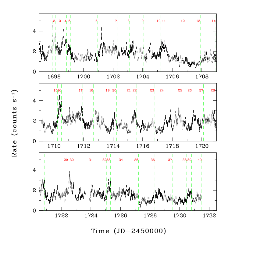
Figure 4: Combined SIS 0.7–1.3 keV light curve in cts s^-1 and in 256 s bins. The background level in the source cell is about 4 % of the source count rate, and not plotted. The vertical dashed lines delineate our 40 time intervals within which spectra were extracted, as described in § 5.

In order to construct a complete picture of the multi-waveband variability of an AGN, one must consider the variations of X-ray spectral parameters. Simple flux-flux correlations can miss important clues to the emission and reprocessing mechanisms at work. In order to study the spectral evolution of Akn 564, we created 40 time-selected spectra across the 35 day observation. We sampled throughout the light curve following flares and dips using Xselect V2.0. The resulting average baseline for each time-selected spectrum was $\sim 75$ ks, and the average on-source exposure time was $\sim 25$ ks. (We note that the spectral variations which we will demonstrate and discuss were also evident when the data were sampled evenly, although such a sampling seemed to average out some interesting fluctuations). Figure 4 shows our choice of intervals as vertical dashed lines plotted over the combined SIS light curve. We set the background, ancillary response, and response matrix files to be those of the mean spectrum, as the background spectrum and flux did not vary significantly during the observation, and we wished to attain the best possible signal-to-noise in the subtracted data. We also grouped the source counts with a minimum of 20 counts per energy bin as before. All fits were performed fixing the scaling factors for instrument normalization among the 4 datasets (SIS and GIS) and the corrections for the SIS low-energy problem (see § 2) to the best-fit values from the mean spectrum. We consistently modified our models with Galactic absorption by a column $N_{\rm H}=6.4\times 10^{20}$ cm^-2. The time stamps of the light curves shown in this section are in JD-2450000 and refer to the mid-point of the observation. Figure 5 shows the results from this analysis, described in full below.

5.2 Variability of the Continuum

For each of the 40 time-selected spectra we fitted the SIS data in the range 2.5–4.88 keV simultaneously with the GIS data in the ranges 1.8–4.88 and 7.32–9.76 keV (all observers frame) using a simple power-law model (the same data exclusions as for the mean fit to the continuum slope, § 4). Figure 5 shows the light curves for the (model) continuum flux and the best-fit photon index $\Gamma$. Significant (see § 7) but small variations are observed in $\Gamma$, which has a full range 2.45–2.72, (i.e. $\Delta\Gamma=0.27$) across the 35 days. Some significant changes are apparent down to timescales of $\sim 1$ day (Figure 5). Fitting the photon indices to a constant model yields $\chi^{2}=67/39\ dof$. In addition to changes in slope, we note that the power-law component dominates the 2–10 keV band, thus rapid flux variations observed down to timescales of $\sim 1000$ s in that band are attributable to flux changes in the power-law continuum.

As an illustrative way of examining these spectral variations we constructed a plot to highlight the different aspects of the spectral evolution. Figure 6 shows ratio plots obtained by comparing the best-fit model for the first spectrum to the following 39 spectra. No fitting was performed. The plot is constructed to illustrate the variations of the spectrum and flux compared to the first day of data. Strong variations in both flux and continuum slope are present, as well as a strongly varying soft hump. We note that the soft hump is always evident above the power-law continuum, although it appears to change in absolute strength and relative to the power law. The data show a hint of variations in the Fe K$\alpha$ line, which we investigate in more detail in § 5.4.

5.3 Variability of the Soft X-ray Hump

To examine the variability of the soft hump we utilized SIS data in the range 0.75–1.7 and 2.5–4.88 keV simultaneously with GIS data in the range 1.0–4.88 and 7.32–9.76 keV (observer’s frame). The lower limit of the SIS was based on the level of agreement achieved between the two CCDs using our methods of correction, as described in § 2. The model was a simple power-law plus a broad Gaussian for the soft hump, with Gaussian peak and width fixed at the values noted in § 4.1, while normalization of the soft hump, plus that of the continuum power law and the power-law slope were all left free. To avoid an overly complex model (which can result in false or local minima being found) we excluded data in the Fe K$\alpha$ regime (4.88-7.32 keV) for these fits. Figure 5 shows the time series for the normalization of the soft hump. The soft hump shows a marked decrease in flux across the 35-day observation. Fitting a constant model to the flux of the soft hump yields $\chi^{2}=870/39\ dof$. The hump shows a flux range of a factor $6.44\pm 3.30$ while the 2–10 keV flux (when binned the same way) has a range of a factor $3.97\pm 0.06$. An alternative measure to the trough-to-peak was obtained by averaging the first and last three of the 40 points for each component, this method avoids the numbers being dominated by a single strong event. This shows that the power-law falls by a factor $1.68\pm 0.01$ and the soft hump by a factor $2.81\pm 0.24$ from the start to the end of the ASCA observation. The different amplitudes of variability of the power-law and hump explain the gross change in softness ratio across the observation (Figure 1). By eye, it is clear that some of the flares in the hard X-ray flux are also evident in the soft hump. We discuss the detailed correlation between X-ray parameters in § 7.

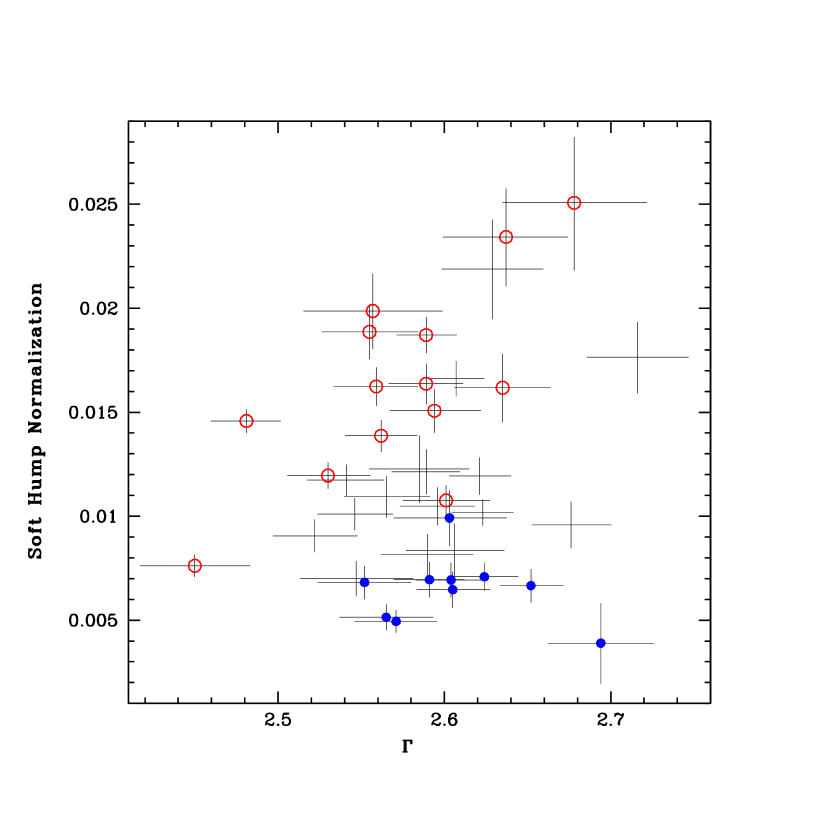
Figure 8: The strength of the soft hump plotted against photon index $\Gamma$, with high-state (open circles) and low states (filled circles) overlaid.

To confirm this result, we split the data into “hard” and “soft” states based upon the softness ratio. We chose T $<10^{6}$ s for our soft-state spectrum, and T $>2.23\times 10^{6}$ s for our hard-state spectrum where T is the time from the start of the observation (see Figure 1). Fits were performed on each state, in the same way as for the 40 individual spectra. Contour plots were generated for the normalization of the soft hump versus the photon index, $\Gamma$. Figure 7 shows the contours for both states, confirming a significant decrease in the strength of the soft hump across the observation. The clear separation of contours illustrates that this is not confused with changes in the photon index, which are too small to explain the observed spectral changes anyway. $\Gamma$ is also plotted against the strength of the soft hump component, showing no evidence for a correlation between the two (Figure 8). Another concern is that one might expect to see an anti-correlation between the fluxes of the hump and power-law if they were difficult to separate in the spectral fit. However, Figure 8 demonstrates that the high-state data have a systematically higher strength for the soft hump than the low-state. This suggests that the two spectral components are well-separated in the fitting process, and that the two components have a close physical connection.

Figure 6 indicates that the hump undergoes changes in shape on timescales down to days, as evident (for example) by comparison of panels for time-cuts 13 and 35. However, the changes are small relative to the variations in flux of the hump, thus our model with fixed shape for the hump parameterizes most of the flux in the hump at each epoch. Thus, the evidence for some variation in hump shape does not compromise our approach in fixing the shape when testing for flux variability.

We performed a final test, to check our result was not due to variations in the SIS soft response on timescales of weeks. While the SIS degradation is thought to be progressing slowly, the accelerated deterioration evident in data taken during calendar year 2000 led us to look to the GIS for confirmation of the variability in the soft hump. Thus we excluded all SIS data below 1 keV, and used the GIS data down to 0.8 keV to determine the hump flux at each of the 40 epochs. This test strongly confirmed our result, that the soft hump flux falls during the course of this observation, and that this cannot be attributed to any instrumental effects in the ASCA data.

5.4 Variability of the Fe Emission Line

In order to investigate the variability of the Fe emission line, we utilized SIS data in the range 2.5–7.32 keV simultaneously with the GIS data in the range 1.8–9.76 keV. The model was a simple power-law plus the best-fitting profile to the Fexxvi K$\alpha$ line using the Kerr geometry, and the Gaussian model to the Fe K$\beta$/Ni K$\alpha$ blend, the latter was linked to the flux of the K$\alpha$ line, using the observed ratio from the mean spectrum. The shape parameters of the Kerr (K$\alpha$) line were assumed to be constant. As a crude test of this assumption, we split the data using an intensity division equivalent to an SIS0 count rate of 2 cts s^-1, that yielded high- and low-state spectra with similar signal-to-noise in each. We then fit for the mean continuum slope as described in § 4 and overlaid the data in the 4.88-7.32 keV band relative to the local power-law slope in each case. The two line profiles are shown as data/model ratios in Figure 9. The profiles appear similar, although there is some evidence for a slightly higher equivalent width in the low state. Using the high and low-state data we calculated contours of line flux versus $\Gamma$. Figure 10 shows overlapping contours, thus this division of the data reveals no evidence for significant flux variability. We return to the variability of the line EW later.

Returning to the 40 time-selected spectra, we fit those data with a model having free parameters of photon index, the normalization of the power law, and the normalization of the line complex (using the shape parameters from the Kerr fit to the mean profile), no model component was included for the soft hump, as the soft-band data were excluded for this test. Figure 5 shows the time series for the K$\alpha$ line. Fits to a constant model yield $\chi^{2}=36/39\ dof$. Thus the line does not show significant changes in flux when sampled on this timescale.

As an alternative test we split the data into 8 intervals, to sample an intermediate timescale of several days per integration. The intervals each cover several of the original 40 time periods as follows: 1–6; 7–10; 11–17; 18–21; 22–26; 27–29; 30–35; 36–40, and were chosen to follow apparent trends in line flux from Figure 5. A model was constructed using the mean Fe line profile complex from § 4.2 and now assuming the line flux also is constant. The soft-band data were excluded, as for all the Fe line fits performed to date, and so the only free parameters in the fit were photon index and normalization of the power law. If the line is a constant flux component on top of the power-law throughout the observation, then by fitting for the local continuum slope and flux in each interval, one should be able to obtain an acceptable fit for each of the eight intervals. Figure 11 shows the data/model for each fit. While some of the spectra show consistency with the mean line flux, several do not. For example, in interval 1, the line flux is significantly lower than the mean, while in interval 2, and 4, it is higher. The shortest timescale on which one can see some indication for line variability is in comparison of the first two intervals (Figure 11), taking the start time of the first interval, and stop time of the second then this constrains the line to arise in a region $<700,000$ light seconds, or $\sim$ 1 light week in size. Taking the intervals with strongest contrast in residuals (1 and 4), we again calculated contours of line strength versus $\Gamma$. Figure 12 shows these contours, which provide supporting evidence for line variability down to timescales of $\sim$ days. As an example, the difference in fit statistic for a line of fixed versus free strength for interval 2 is $\Delta\chi^{2}=14$, indicating the variability in line flux to be significant at $>$ 99 % confidence.

This result is supported by comparison of the Fe K$\alpha$ line in the soft-state versus hard-state data (defined in § 5.3); a significant difference in line flux and EW is evident between those two states. For the soft-state we found EW${}_{\rm soft}=491^{+103}_{-95}$ eV, with line normalization $n_{\rm soft}=6.2^{+1.5}_{-1.2}\times 10^{-5}$ photons s^-1 cm^-2; for the hard-state EW${}_{\rm hard}=887^{+97}_{-114}$ eV, $n_{\rm hard}=9.6^{+1.1}_{-1.2}\times 10^{-5}$ photons s^-1 cm^-2. This variation cannot be an artifact of confusion with a change in photon index, as the soft and hard states are defined by the strength of the soft hump, and apparently unrelated to $\Gamma$. This result confirms that the line flux and equivalent width both vary during this ASCA observation. There cannot be a simple correlation between soft hump flux and Fe line strength, if that was the case, we would expect to see a gradual decrease in line strength (in Figure 11) as the hump strength went down dramatically across the observation; a correlated drop in line strength is not observed. We note the appearance of some absorption-type features at some epochs (e.g. interval 2), we do not investigate these apparent minor changes to line profile, as such small effects are best investigated when the final ASCA calibration is made available.

6 RMS Spectra

In optical/UV spectroscopy of AGN, it is easy to obtain a series of spectra of sufficiently high S/N to perform time-resolved spectroscopic analysis. In this case, a useful way to isolate variable features is to construct a root-mean-square (rms) spectrum. This ASCA long look has allowed us to use our 40 individual time-selected spectra described in § 5 in analogous way. For each detector the 40 spectra have been rebinned so that each bin has at least a 5-sigma detection (but up to a maximum of 10 adjacent bins were combined to achieve a signal-to-noise ratio of 5 within a bin) then they were degraded to the resolution of the worst spectrum (i.e. the spectrum with worst S/N determined the actual bin widths for them all). We created mean and rms spectra by calculating the simple mean and rms flux in each bin. The choice of a simple mean as opposed to a weighted mean was dictated by the fact that we did not want to weigh in favor of high state spectra.

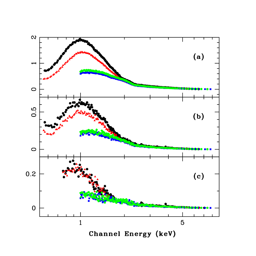
Figure 13: The top panel shows the mean spectrum obtained from our 40 time-selected spectra (in units of counts s^-1 keV^-1, errorbars in the vertical direction are included); the middle panel shows the rms spectrum, that isolates the variable parts of the spectrum; the bottom panel shows the rms spectrum after the power-law continuum is subtracted. Circles refer to the SIS-0 spectrum; triangles to the SIS-1; squares to the GIS-2; pentagons to the GIS-3.

The top panel in Figure 13 shows the mean spectrum, the middle panel, the rms spectrum. The bottom panel shows the rms spectrum after the power-law continuum is subtracted (hence only the energy bands used in the fits are plotted). This shows that the most pronounced variability occurs in the soft-X band, consistent with our results of § 3.1, and that the variations in the Fe line are of low significance with this division of the data into 40 intervals.

7 Cross-correlation Results

The X-ray light curves in different energy bands (Figure 1) exhibit visually similar characteristics, suggesting a short time delay between the variations in each curve. In order to quantify any correlations, we undertook a cross-correlation analysis using the interpolation cross-correlation function (ICCF) method of Gaskell & Sparke (1986) and Gaskell & Peterson (1987) as implemented by White & Peterson (1994).

We first considered a simple flux–flux correlation. We calculated the CCFs of the total hard-flux in the 2–10 keV band with respect to the total soft-flux in the 0.7–1.3 keV band (binned to 5760 s). The maximum value of the correlation coefficient is $r_{\rm max}=0.942$ and the ICCF centroid $\tau_{\rm cent}=0.012^{+0.003}_{-0.011}$ d, less than 0.02 d at 95 % confidence. The CCF is sampled at a resolution of 0.005 day, and the centroids are computed using all points near the peak of the CCFs with values greater than 0.8 $r_{\rm max}$. The 1-$\sigma$ uncertainties quoted for $\tau_{\rm cent}$ are based on the model-independent Monte Carlo method described by Peterson et al. (1998). Given the $\sim$ 500 points in our light curves, there is a $\ll$ 0.1 % chance of exceeding $r_{\rm max}\approx 0.3$ from uncorrelated samples. The power-law component provides $\sim$ 75 % of the flux in the 0.7–1.3 keV band (in the mean spectrum) and so rapid variability in the power-law flux is dominating the soft/hard flux correlation. To understand the physics, we also need to examine the spectroscopically-separated components.

The cross-correlations between X-ray spectral parameters are summarized in Table 1. We calculated the CCFs of the light curves listed in Column (1) of Table 1 relative to the light curves shown in the first line, namely, the hard X-ray continuum, the soft X-ray hump, and the photon index $\Gamma$. The maximum value of the correlation coefficient $r_{\rm max}$ and the ICCF centroid $\tau_{\rm cent}$ relative to the hard X-ray continuum are given in Columns (2) and (3); the ones relative to the X-ray soft hump are given in Columns (4) and (5); and the ones relative to the photon index are given in Columns (6) and (7), respectively. The CCFs are defined such that a positive lag means that the light curves listed in Line (1) of Table 1 are leading the light curves listed in Column (1). The number of points in the X-ray light curves is 40; the number of points in the overlapping portion of the X-ray and 1365 Å light curves is 34. The CCFs are sampled at a resolution of 0.1 day, and the centroids are computed using all points near the peak of the CCFs with values greater than 0.8 $r_{\rm max}$. The 1-$\sigma$ uncertainties quoted for $\tau_{\rm cent}$ are based on the model-independent Monte Carlo method described by Peterson et al. (1998). For our 40 points there is a 0.1 % chance of exceeding $r_{\rm max}=0.5$ from uncorrelated samples. Figure 5 shows the light curves and the CCFs calculated relative to the hard X-ray continuum, and the hard X-ray continuum autocorrelation function (ACF).

We see a strong correlation with no significant lag between the 2–10 keV flux and soft hump flux. The soft hump flux is distinct from the total soft-band flux (which is the sum of power law plus soft hump counts), as it was obtained by spectral fitting. The use of quantities derived from spectral fitting limits the finest time resolution to $\sim$ a day. The correlation is good because events on timescales of $\sim$ a day occur in both the hump and power-law components. Also, while the soft hump shows a $\sim$ 50 % stronger decline over the 35 day observation than that which occurs in the 2–10 keV flux, both components show a gradual correlated decline. We also showed that the power-law flux varies down to timescales of $\sim 1000$ s and rapid changes in softness ratio (Edelson et al., 2001) indicate this occurs without a comparable change in the soft hump. Thus the strength of the correlation between the spectral components depends on the timescale of sampling.

The final panel of Figure 5 compares the UV light curve at 1365 Å with the hard X-ray flux. The correlation is strong, and the lag of the UV relative to the hard X-rays is consistent with $\sim$ 0, with an upper limit of 1.0 d at 95 % confidence. The Fe K$\alpha$ line does not show significant correlations with any X-ray quantity (and thus is not shown in the Table or Figure) as the error on each of the 40 measurements is very large. It is also important to note that $\Gamma$ is not well correlated with the UV flux or the soft hump flux (Table 1), ruling out simple models where a steepening of the photon index can explain observed properties in the UV and soft X-ray regimes.

The strong correlation between the hard X-ray and UV curves leads us to make a direct comparison of the soft hump flux and UV light curve. The CCF of 1365 Å  relative to the soft X-ray hump is shown in Figure 14. There is a good correlation between soft hump and UV 1365 Å flux, with the UV–soft hump lag consistent with 0 days and less than 1.0 d at 95 % confidence. Most notably, the bright X-ray flare around day 1710 is evident in the hard X-ray, soft hump and UV light curves. The difference between the correlation coefficients obtained for the hard-flux–1365 Å  versus hump–1365 Å is not significant, so we cannot distinguish which is the primary link.

8 Summary of Observational Results

• Akn 564 shows flux variations by factors up to 16 in the 0.7–1.3 keV band, 14 in the 2–10 keV band when sampled on 256 s timescales over a 35-day baseline.

• Fractional variability amplitude changes with time with no clear correlations with flux or spectral parameters.

• The mean photon index is $\Gamma\sim 2.54$ in the hard band, with variations of $\Delta\Gamma=0.27$ and significant changes observed down to a timescale of $\sim$ a day.

• A separate soft hump component detected below 1 keV is found to be variable down to timescales of $\sim$ a day, ranging by a factor of $\sim$ 6 in normalization over the observation, but always being present. Some changes in hump shape are evident down to timescales of days.

• The photon index does not appear to be significantly correlated with any of the other X-ray parameters and is not confused with soft hump strength.

• The powerlaw and hump are not well correlated on timescales of 1000 s Sharp variations occur in the power-law component, but examination of the softness ratio during those times (Edelson et al., 2001) indicates that comparable rapid changes do not occur in the soft hump flux.

• The soft hump shows $\sim$ 50 % larger variation in amplitude than the power-law component over a baseline of weeks, when sampled $\sim$ daily. This difference causes changes in the softness ratio across the observation.

• The UV 1365 Å flux is well correlated with the soft hump and hard X-ray flux. Correlated events (of different amplitudes) appear in all three light curves on timescales of $\sim$ a day. We detect no significant lag between the UV and X-ray bands.

• Fe K$\alpha$ emission is detected in addition to a line representing a blend of Fe K$\beta$ emission and Ni K$\alpha$, all from H-like ions, confirming that the reprocessor is highly ionized.

• The flux and EW of the Fe K$\alpha$ line vary, down to timescales of $\sim$ a week.

9 Discussion and Conclusions

Akn 564 shows large amplitude and rapid X-ray variability, with a trough-to-peak range of a factor of $\sim$ 16 sampled in the 0.7–1.3 keV band using 256 s bins over this 35 day ASCA observation. The 2–10 keV band also shows rapid and large amplitude variability with a maximum range a factor of 14 (using 256 s bins) and factors of $\sim$ several change over a few thousand seconds. While the fractional variability changes with time, this does not appear to be well correlated with flux. Furthermore, the fractional variability does not appear to be correlated with any X-ray, UV or optical parameter at zero lag (see Paper III for the X-ray–optical correlations, Shemmer et al., 2001). It is difficult to understand the apparent lag of the peak in flickering behavior ($F_{\rm var}$ lags by 3 days relative to the big X-ray flares). The BLS1 NGC 7469 also shows variations in $\sigma^{2}_{\rm rms}$ which do not appear to correlate with X-ray spectral parameters of UV flux in any clear way. Akn 564 does not show the strong anti-correlation between fractional variability and UV flux indicated for NGC 7469 (Nandra et al., 2000).

The photon index $\Gamma\sim 2.54$ is steep for a NLS1 galaxy compared to measurements of other such sources (Brandt, Mathur, & Elvis, 1997; Turner, George, & Nandra, 1998; Leighly, 1999b; Vaughan et al., 1999b). The photon index varies between 2.45–2.72, comparable to the variability in $\Gamma$ observed in the BLS1 NGC 7469 ($\Delta\Gamma=0.32$, Nandra et al., 2000). This may indicate that the disk corona shows a similar degree of fluctuation in temperature and/or optical depth in BLS1s and NLS1, although the absolute conditions appear to be very different. In contrast to NGC 7469, there appears to be no correlation between photon index and UV flux (Figure 5). In addition, the extrapolation of the hard X-ray power law overpredicts the UV and optical fluxes (Walter & Fink, 1993). Thus the hard X-ray power law does not appear to simply extrapolate into the UV band in Akn 564, and the component must terminate or turn over at wavelengths shorter than 1365 Å.

A distinct soft hump is observed in addition to the power-law continuum. The component rises above the power-law below 2 keV, and shows a distinct spectral flattening below 1 keV, rising again below 0.5 keV. This hump was first detected in an earlier ASCA observation of Akn 564 (Turner, George, & Netzer, 1999a). The soft hump shows flares which are correlated with those in the power-law component, down to timescales of days (the shortest timescale we can reliably probe the hump spectroscopically using these data), the flares are not generally of the same amplitude in the soft and hard bands. There is a distinction in the soft hump and power-law variability over a timescale of weeks, with the former varying by a factor of $\sim 6$ across the 35-day baseline of the observation compared to a factor 4 in the power-law (when sampled $\sim$ daily). This difference in amplitudes of variation causes changes in the softness ratio across the observation.

We can infer something about the rapid variability of the hump only by using an indirect method. Some spectral changes on timescales of $\sim$ 1000 s (Edelson et al., 2001) are clearly due to sharper changes in hard than soft X-ray flux suggesting the soft hump does not vary as fast as the power-law. In this case, the overall larger measure of $F_{\rm var}$ in the soft band is most likely due to the relatively strong changes in hump-flux on timescales of weeks.

We note that the pronounced variability of the soft hump immediately rules out an origin as starburst emission. Chandra results from another NLS1, TonS180 (Turner et al., 2001), have shown no absorption lines, indicating the shape of the hump in that case is unlikely to be due to a combination of absorption effects and a steepening continuum form. Akn 564 is more likely to show a soft component which is modified in shape by absorption, as the UV data indicate the presence of a column $\sim 9\times 10^{20}{\rm cm^{-2}}$ (Crenshaw et al., 2001). However, the fact that the ASCA spectra of Akn 564 and TonS180 look very similar has led us to consider the soft hump in Akn 564 likely to be a continuum component or broadened reprocessed component from the accretion disk, as suggested for TonS180. Collinge et al. (2001) find a soft hump in NGC 4051 of similar form to that in Akn 564 and TonS180 and this may also be attributable to a smooth continuum-like component. This good correlation between the UV flux and the soft hump and the upper limit to the lag of $\sim 1$ d indicates a contribution to both bands by the same physical component, perhaps emission from the accretion disk. The UV/soft hump correlation and the apparent association of the soft hump with NLS1s appears consistent with the idea that the disk peaks at a higher temperature in NLS1s than BLS1s, as expected if we are viewing thermal emission from a disk which is more highly ionized in the NLS1 case (Ross, Fabian, & Mineshige, 1992). Unfortunately these data do not allow us to distinguish whether the soft hump is due to reflected radiation from an ionized disk, thermal emission from the disk or a combination of both. The changes in the shape of the hump may indicate that it is the superposition of several different components of emission/reflection, which possess differing timescales of variability.

In general, we find disk-corona models to be challenged by the lack of correlation of $\Gamma$ with the strength of the soft hump, presumably the seed photon source, which should cool the corona and cause a steepening in the power law as it increases in strength. One possibility is that the corona cooling is saturated, i.e. that even a significant reduction in the soft hump leaves a large enough soft-photon reservoir that the resulting spectrum is always strongly cooled. We defer a more detailed discussion of the multiwaveband lags and correlations, and reprocessing models, to Paper III (Shemmer et al., 2001).

An Fe K$\alpha$ line of high equivalent width is detected and clearly attributable to highly ionized material. These are strong observational results which are robust to the current inaccuracies in calibration. Analysis using the current calibration suggests a dominance of Fexxvi ions in Akn 564 (yielding Ly$\alpha$), although a blend of emission from several states is most likely. An additional line of equivalent width $63^{+54}_{-38}$ eV is detected, close to a rest energy of 8.2 keV. Lines consistent with this energy are the K$\beta$ line from H-like Fe (Ly$\beta$) and the K$\alpha$ line from H-like Ni (Ly$\alpha$). Assuming solar abundances then the predicted equivalent width of Fe K$\beta$ is 77 eV, and that of Ni K$\alpha$ is 35 eV, based on the strength of the Fe K$\alpha$ line. Thus we attribute the line at 8.2 keV to a blend of these two, and the total observed equivalent width is consistent with such a sum. A previous short ASCA observation of Akn 564 showed ambiguity between ionization-state of the reprocessor and inclination angle of the disk system (Turner, George, & Netzer, 1999a), however, these data show that an ionized reprocessor is clearly present in this source. The discovery of ionized reprocessors in some BLS1s (e.g., Guainazzi et al., 1998) indicates that the luminosity of the central source may be as important as accretion rate in creating an ionized surface to the disk.

The equivalent widths for the Fe lines are huge (with EW$=653\pm 85$ eV for Ly$\alpha$) compared to those observed in Seyfert 1 galaxies (e.g. Nandra et al., 1997a). Similarly large values have been noted in previous ASCA observations of this and other NLS1s (Turner, George, & Nandra, 1998; Comastri et al., 1998). The large EWs may be partly explained by the relatively large line fluxes expected from He-like and H-like ions compared to neutral material. Another possibility is that NLS1s have high Fe abundance. Noting the high EWs of Fe K$\alpha$ and the strong Feii emission in NLS1s Turner, George, & Netzer (1999a) suggested that high Fe abundance might be a general property of NLS1s; furthermore, high metallicities are expected in some evolutionary models for NLS1s (Mathur, 2000). The high EW cannot be due to a large solid angle for the reprocessor or a hidden hard X-ray component, as, in either of these cases we would observe a detectable flattening to high energies due to the presence of the associated Compton hump. The ASCA data show variations in the Fe K$\alpha$ flux by a factor $\sim 2.4$ on timescales $<7\times 10^{5}$ light seconds, indicating the bulk of the iron line originates within $\sim$ a light week of the nucleus.

Figure 1: Light curves for the ASCA data taken between 2000 June 1 and July 6, in cts s^-1 and in 5760 s bins. The top panel is the SIS soft band (0.7–1.3 keV) light curve; the middle panel the GIS hard band (2–10 keV) and the bottom panel is the ratio of 0.7–1.3/2–10 keV. The background level in the source cell is about 4 % of the source count rate, and not plotted. The times are reported both in seconds from the start of exposure (top axis) and in JD-2450000 (bottom axis). The horizontal lines show the periods referred to as the soft and hard states.

Figure 2: Data/Model where the model is a simple power law fit to the 2–5 plus 7.5–10 keV data (rest-frame). The rest of the ASCA data are then overlaid, revealing a strong soft hump and Fe emission line. The data used in our spectral analysis are shown as filled circles, the data disguarded due to problems with the current ASCA calibration are overlaid, as open circles. The inset panel shows the ROSAT PSPC data compared to the continuum power-law, demonstrating the shape of the soft hump to lower energies.

Figure 3: Data/Model where the model is a power law plus soft hump plus Kerr model for the Fe K$\alpha$ line. The data show the presence of an additional component, due to a blend of Fe K$\beta$ and Ni K$\alpha$ emission at a rest-energy $\sim$ 8.2 keV.

Figure 5: Spectral and timing parameters obtained from fits to the individual time-resolved spectra (left-hand column) and CCFs (right-hand column, discussed in § 7). From the top, the light curves are the model continuum flux in the hard band, the photon index $\Gamma$, the soft hump normalization, the ${\rm K}\alpha$ normalization, the fractional variability $F_{\rm var}$ in the soft and hard bands, the continuum flux at 1365 Å from Collier et al. (2001). The X-ray continuum fluxes are in units of $10^{-11}$ ergs s^-1 cm^-2, the soft hump normalization and the ${\rm K}\alpha$ normalization are in units of $10^{-4}$ photons s^-1 cm^-2, the UV continuum in units of $10^{-15}$ ergs s^-1 cm^-2. The CCFs are calculated relative to the hard X-ray continuum (top, left), and the top panel on the right is the hard X-ray continuum ACF.

Figure 6: Ratio plots obtained by fitting the best-fit model for the first spectrum to the following 39 spectra. Energy ranges and instrument utilized are described in § 5.2.

Figure 7: The $\Delta\chi^{2}=2.3,4.61,9.21$ contour levels for the soft hump normalization (in units photons s^-1 cm^-2) vs. photon index $\Gamma$. The dashed contours correspond to the soft state, the full contours to the hard state, and the best-fit values are indicated by crosses.

Figure 9: Data from the Fe K regime compared to the continuum model, with high-state (open circles) and low states (filled circles) overlaid.

Figure 10: The $\Delta\chi^{2}=2.3,4.61,9.21$ contour levels for Fe K-shell line intensity (in units photons s^-1 cm^-2) vs. photon index $\Gamma$. The dashed contours correspond to the low state, the full contours to the high state, and the best-fit values are indicated by crosses.

Figure 11: Data from the Fe K regime compared to the continuum model plus fixed line profile from the mean spectrum, sampled every few days. The systematically high or low residuals indicate line variability, see § 5.4 for more details.

Figure 12: The $\Delta\chi^{2}=2.3,4.61,9.21$ contour levels for Fe K shell line intensity (in units photons s^-1 cm^-2) vs. photon index $\Gamma$. The dashed contours correspond to interval 1 the full contours to interval 4, as described in § 5.4.

Figure 14: Light curves (left-hand column) and CCFs (right-hand column). From the top, the light curves are the X-ray soft hump normalization, and the UV continuum at 1365 Å. The X-ray soft hump normalization is in units of ${\rm photons\ s}^{-1}\;{\rm cm}^{-2}$, and the UV fluxes in units of $10^{-15}$ ergs s^-1 cm^-2 Å^-1. The CCF is calculated relative to the X-ray soft hump (top, left), and the top panel on the right is the X-ray soft hump ACF. Positive peaks mean that the X-ray soft hump is leading. UV data from Collier et al. (2001).

Table 1: X-Ray and UV Cross-Correlation Results

	F${}_{2-10\;\,{}{\rm keV}}$		Soft Hump		$\Gamma$
	$r_{\rm max}$	$\tau_{\rm cent}$	$r_{\rm max}$	$\tau_{\rm cent}$	$r_{\rm max}$	$\tau_{\rm cent}$
(1)	(2)	(3)	(4)	(5)	(6)	(7)
$\Gamma$	0.389	-0.05${}^{+0.10}_{-0.35}$	0.058	0.00${}^{+0.04}_{-0.59}$	$\cdots$	$\cdots$
Soft Hump	0.675	0.00${}^{+0.20}_{-0.10}$	$\cdots$	$\cdots$	$\cdots$	$\cdots$
$F_{\rm var}$ (0.7–1.3 keV)	0.584	$2.94^{+0.31}_{-0.15}$	0.232	3.00${}^{+1.10}_{-0.15}$	0.153	-0.95${}^{+2.25}_{-0.84}$
$F_{\rm var}$ (2–10 keV)	0.557	$2.85^{+0.30}_{-0.10}$	0.405	3.05${}^{+2.26}_{-0.10}$	0.239	-0.00${}^{+3.89}_{-5.54}$
Fλ (1365 Å)	0.683	0.39${}^{+0.26}_{-0.84}$	0.633	0.35${}^{+0.35}_{-0.44}$	0.112	$0.70^{+0.30}_{-0.30}$

References

- Ballantyne, Iwasawa, & Fabian (2000) Ballantyne, D. R., Iwasawa, K., & Fabian, A. C. 2000, MNRAS, in press (astro-ph/0011360)
- Blandford & McKee (1982) Blandford, R., & McKee, C. 1982, ApJ, 255, 419
- Boller, Brandt, & Fink (1996) Boller, Th., Brandt, W. N., & Fink, H. 1996, A&A, 305, 53
- Boller, Brandt, & Fabian (1997) Boller, Th., Brandt, W. N., & Fabian, A.C. 1997, MNRAS, 289, 293
- Boroson & Green (1992) Boroson, T. A. & Green, R. F. 1992, ApJS, 80, 109
- Brandt et al. (1994) Brandt, W. N., Fabian, A. C., Nandra, K., Reynolds, C. S., & Brinkmann, W. 1994, MNRAS, 271, 958
- Brandt, Mathur, & Elvis (1997) Brandt, W. N., Mathur, S., & Elvis, M. 1997, MNRAS, 285, L25
- Brandt et al. (2001) Brandt, W. N., et al. 2001, in preparation
- Burke et al. (1991) Burke, B. E., Mountain, R. W., Harrison, D. C., Bautz, M. W., Doty, J. P., Ricker, G. R., Daniels, P. J. 1991, IEEE Trans. ED-38, 1069
- Collier et al. (2001) Collier, S. J., et al. 2001, ApJ, submitted (Paper II)
- Collinge et al. (2001) Collinge, M. J., Brandt, W. N., Kaspi, S., Crenshaw, D. M., Elvis, M., Kraemer, S. B., Reynolds, C. S., Sambruna, R., Wills, B., 2001, ApJ, submitted
- Comastri et al. (1998) Comastri, A., et al. 1998, A&A, 333, 31
- Comastri et al. (2001) Comastri, A., et al. 2001, A&A, in press (astro-ph/0010476)
- Crenshaw et al. (2001) Crenshaw, M., et al. 2001, in preparation
- de Vaucouleurs et al. (1991) de Vaucouleurs, G., de Vaucouleurs, A., Corwin, H. G., Buta, R. J., Paturel, G., & Fouque, P. 1991, S&T, 82, 621
- Dickey & Lockman (1990) Dickey, J. M., & Lockman, F. M. 1990, ARA&A, 28, 215
- Edelson et al. (2001) Edelson, R., et al. 2001, in preparation
- Fabian et al. (1989) Fabian, A. C., Rees, M. J., Stella, L., & White, N. E. 1989 , MNRAS, 238, 729
- Forster & Halpern (1996) Forster, K. & Halpern, J. 1996,ApJ, 468, 565
- Gaskell & Sparke (1986) Gaskell, C. M., & Sparke, L. S. 1986, ApJ, 305, 175
- Gaskell & Peterson (1987) Gaskell, C. M., & Peterson, B. M. 1987, ApJS, 65, 1
- Goodrich (1989) Goodrich, R. W. 1989, ApJ, 342, 234
- Guainazzi et al. (1998) Guainazzi, M., Piro, L., Capalbi, M., Parmar, A.N., Yamaguchi, M., & Matuoka, M. 1998, A&A, 339, 327
- Guilbert, Fabian, & McCray (1983) Guilbert, P. W., Fabian, A. C., & McCray, R. 1983, ApJ, 266, 466
- Huchra, Vogeley & Geller (1999) Huchra, J. P., Vogeley, M. S., & Geller, M. J. 1999, ApJS, 121, 287
- Kaspi et al. (2000) Kaspi, S., Smith, P. S., Netzer, H., Maoz, D., Jannuzi, B. T., & Giveon, U. 2000, ApJ, 533, 631
- Laor (1991) Laor, A. 1991, ApJ, 376, 90
- Laor et al. (1997) Laor, A., Fiore, F., Elvis, M., et al. 1997, ApJ, 477, 93
- Leighly (1999a) Leighly, K. M. 1999a, ApJS, 125, 297
- Leighly (1999b) Leighly, K. M. 1999b, ApJS, 125, 317
- Maraschi & Haardt (1997) Maraschi, L., Haardt, F. 1997, in IAU Colloq. 163, Accretion Phenomena and related Outflows, ed. D. Wickramasinghe, L. Ferrario, & G. Bicknell, Publ. Astron. Soc. of Australia Press
- Mathur (2000) Mathur, S. 2000, MNRAS, 314, L17
- Matt, Fabian, & Ross (1993) Matt, G., Fabian, A. C., & Ross, R.R. 1993, MNRAS, 264, 839
- Nandra et al. (1997a) Nandra, K., George, I. M., Mushotzky, R. F., Turner, T. J., & Yaqoob, T. 1997a, ApJ, 477, 602
- Nandra et al. (1997b) Nandra, K., George, I. M., Mushotzky, R. F., Turner, T. J., & Yaqoob, T. 1997b, ApJ, 476, 70
- Nandra et al. (2000) Nandra, K., Le, T., George, I. M., Edelson, R. A., Mushotzky, R. F., Peterson, B. M., & Turner, T. J. 2000, ApJ, 544, 734
- Ohashi et al. (1996) Ohashi, T., et al. 1996, PASJ, 48, 157
- Osterbrock & Pogge (1985) Osterbrock, D. E., & Pogge, R. W. 1985, ApJ, 297, 166
- Peterson (1993) Peterson, B. M. 1993, PASP, 105, 207
- Peterson et al. (1998) Peterson, B. M., Wanders, I., Horne, K., Collier, S., Alexander, T., Kaspi, S., & Maoz, D. 1998, PASP, 110, 660
- Peterson et al. (2000) Peterson, B. M. et al. 2000, ApJ, 542, 161
- Pounds, Done, & Osborne (1995) Pounds, K. A., Done, C. & Osborne, J. P. 1995, MNRAS, 277, L5
- Pounds et al. (2001) Pounds, K. A., Edelson, R., Markowicz, A., & Vaughan, S. 2001, ApJ, in press (astro-ph/0101542)
- Rodriguez-Ardila et al. (2000) Rodriguez-Ardila, A. Binette, L., Pastoriza, M. G., Donzelli, C. J. 2000, ApJ, 538, 581
- Ross, Fabian, & Mineshige (1992) Ross, R., Fabian, A. C., & Mineshige, S. 1992, MNRAS, 258, 189
- Shemmer et al. (2001) Shemmer, O., et al. 2001, ApJ, submitted (Paper III)
- Turner, George, & Nandra (1998) Turner, T. J., George, I. M., & Nandra, K. 1998, ApJ, 508, 648
- Turner, George, & Netzer (1999a) Turner, T. J., George, I. M., & Netzer, H. 1999, ApJ, 526, 52
- Turner et al. (2001) Turner, T. J., et al. 2001, ApJ, 548, L13
- Turner et al. (1999b) Turner, T. J., et al. 1999b, in Proceedings of the 19th Texas Symposium on Relativistic Astrophysics and Cosmology, ed. J. Paul, T. Montmerle, & E. Aubourg (Saclay: CEA), E441
- Vaughan et al. (1999a) Vaughan, S., Pounds, K. A., Reeves, J., Warwick, R., & Edelson, R., 1999, MNRAS, 308, L34
- Vaughan et al. (1999b) Vaughan, S., Reeves, J., Warwick, R., & Edelson, R. 1999, MNRAS, 309, 113
- Walter & Fink (1993) Walter, R. & Fink, H. H. 1993, A&A, 274, 105
- Wandel, Peterson & Malkan (1999) Wandel, A., Peterson, B.M., & Malkan, M. 1999, ApJ, 526, 579
- White & Peterson (1994) White, R. J., & Peterson, B. M. 1994, PASP, 106, 879
- Yaqoob et al. (2000) Yaqoob, T., et al. 2000, ASCA GOF Calibration Memo, ASCA-CAL-00-06-01, v1.0