Four Extreme Relic Radio Sources in Clusters of Galaxies

Abstract

We describe the results of the highest-resolution radio observations yet made of four relic radio sources in the Abell clusters A13, A85, A133 and A4038. Our VLA images at 1.4 GHz with 4^′′ resolution and a noise level of 1 $\sigma\sim$ 20 $\mu$Jy beam^-1 (1.1 K) show a remarkable variety of fine structure in the form of spectacular arcs, wisps, plumes and loops. Their integrated radio flux densities fall very rapidly with frequency, with power-law slopes, $\alpha$, between 2.1 and 4.4 near 1.4 GHz (where $S_{\nu}\propto(\nu/\nu_{0})^{-\alpha}$). The relics possess linear polarization levels ranging between 2.3 % (A133) and 35 % (A85); the higher polarization fractions imply a highly ordered magnetic field in the fine structure and low differential Faraday rotation in the intervening cluster gas.

The optical identification of a host galaxy formerly associated with a relic remains problematic. In A85, A133 and A4038 the travel times for the brightest cluster galaxies are significantly longer than the modeled ages of the relics; there is always at least one nearby relatively bright elliptical that provides a better match.

Excess X-ray emission in the 0.5 keV-to-2 keV band was found near the relics in A85 and A133. The surface brightness was too high to be attributed to the inverse-Compton mechanism alone.

We found excellent fits to the broad-band radio spectra using the anisotropic (KGKP) model of spectral ageing, and we have extended the model to include diffusion of particles between regions of different field strength (the Murgia-JP, or MJP, model). The steep radio spectra imply ages for the relics of $\sim 10^{8}$ yr, at the start of which period their radio luminosities would have been $\sim 10^{25}$ W Hz^-1 at 1.4 GHz, and so their progenitors were on the boundary between FR I and FR II radio galaxies and hence among the most luminous 7 % of radio galaxies.

We find that the relics are in approximate pressure equilibrium with the surrounding intra-cluster gas, which has probably limited their free expansion and prevented them from fading by adiabatic cooling.

1 Introduction

About one in ten rich clusters of galaxies observed with comparatively low-resolution radio telescopes contains a diffuse steep-spectrum source with no optical identification (Giovannini, Tordi & Feretti 1999). Some of these sources take the form of a halo near the cluster centre with a diameter of 1 Mpc to 2 Mpc; the prototype is the halo in the Coma cluster (Willson 1970). Others with various morphologies (sometimes arc-like or with multiple components) are situated further from the cluster centre (Slee & Reynolds 1984) or even out near the cluster perimeter (Röttgering et al. 1997); such non-central sources are termed “relics”. In the clusters Coma (Enßlin et al. 1998), A1300 (Reid et al. 1999), A2255 (Feretti et al. 1997), A2744 (Govoni et al. 2001) and possibly in the cluster 1E 0657$-$56 (Liang et al. 2000), both a halo and a relic have been found.

Recently, Slee & Roy (1998) found much fine structure at 4^′′ resolution in the relic in A4038. This relic is most likely the remnant of a radio galaxy whose progenitor is now some 18 kpc to the relic’s east, though surprisingly the structure does not look like a relaxed plasma in which no further electron reacceleration is taking place.

Various schemes for the production of halos and relics include the remnants of de-energised radio galaxies, adiabatic recompression of old, expanded radio lobes (Enßlin & Gopal-Krishna 2001), the turbulent wakes of galaxies that once passed through the region, reacceleration of electrons in shock fronts caused by cluster mergers, and reacceleration of electrons in shocks caused by the accretion of gas by the cluster potential. Most of these proposals possess the common feature that adiabatic expansion of the radio plasma has been prevented by the pressure of the hot intra-cluster gas for $\sim$ 10⁸ yr, allowing the inverse-Compton and synchrotron losses to steepen the electron-energy spectrum and thus the radio spectrum (Goldshmidt & Rephaeli 1994). Detailed modeling of the spectral evolution can then yield estimates of the relic’s age and magnetic field strength and, if a direct detection of the inverse-Compton X-rays is made, of the magnetic field strength independent of the usual equipartition arguments.

This paper describes the results of further higher-resolution observations with the Very Large Array (VLA) of the relics A13_6a/b/c, A85_25a/b/c and A133_7a/b. These relics were first identified in the VLA and Molonglo Observatory Synthesis Telescope (MOST) maps of Slee & Reynolds (1984), who demonstrated their extremely steep ($\alpha\geq\,$2) spectra and lack of optical host galaxies (where S${}_{\nu}\propto(\nu/\nu_{\circ})^{-\alpha}$). Better VLA images were presented by Slee, Roy & Savage (1994) of these and other relics that were found during their survey of 58 clusters drawn from the Abell cluster sample (Abell, Corwin Jr., & Olowin 1989). Here, we present new images at 4^′′ resolution of three of these relics, which is the highest resolution yet achieved in imaging such sources, and give further measurements from the images of A4038_9 (Slee & Roy 1998). Basic properties of the clusters are given in Table 1, where the nomenclature is that of Slee, Roy & Savage (1994).

Throughout this paper we adopt $H_{\circ}$ = 75 km s^-1 Mpc^-1 and $q_{\circ}$ = 0.5.

2 The Observations

We observed the four relics with the VLA at 1.425 GHz in the BnA configuration (A13, A133, A4038) or the B configuration (A85) for 8 h and 9 h, respectively. A13 and A133 were observed on 1998 June 25, A85 on 1998 September 1 and A4038 on 1997 January 26. We obtained higher resolution (4^′′) than that of our earlier survey observations (15^′′) (Slee, Roy & Savage 1994). We used four 50 MHz bands, recording left- and right- and cross-circular polarization products. Calibration and imaging were done with AIPS, using standard methods. The flux-density scale was calibrated assuming that 3C 48 had flux densities of 16.36 Jy at 1.385 GHz and 15.67 Jy at 1.465 GHz. The polarization calibrators were 3C 286 for A13 and A133 and 3C 138 for A85 and A4038. Nearby phase calibrators were observed every 35 min throughout the observation for initial phase calibration. The data were then self-calibrated and separate images were made for the two frequency bands using uniform and natural weighting. The dirty images were deconvolved using the CLEAN algorithm, with component subtraction from the ungridded ($u$, $v$) data as implemented in the AIPS task MX, and the images were restored using beams of $\sim$ 4^′′ and $\sim$ 6^′′ for the uniformly- and naturally-weighted images, respectively. The $1\,\sigma$ noise in the final images ranged from 17 $\mu$Jy beam^-1 to 21 $\mu$Jy beam^-1 in a 4^′′ beam (1.0 K to 1.2 K), which is $\sim$ 50 % above the thermal noise limit.

To measure the spectral index, we used flux densities from the 1.385 and 1.465 GHz images which, although closely spaced in frequency, yielded useful values of spectral index for these steep spectrum sources.

The ($u$, $v$) data were polarization-calibrated, and polarized intensity images were made from the resulting images of Stokes parameters Q and U. The instrumental polarization varies with time, limiting the minimum believable polarization fraction to nominally 0.15% for the VLA.

3 Results

3.1 Radio Images

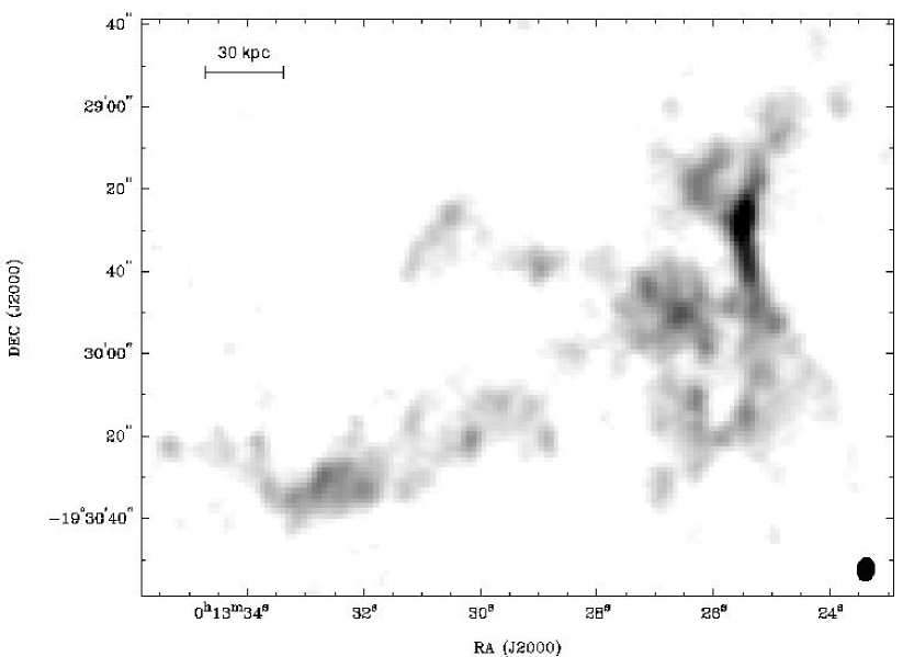
Figure 1: VLA naturally-weighted image of the relic in A13 at 1.425 GHz. The FWHM restoring beam in the lower right corner is 5.9${}^{\prime\prime}\times 4.4^{\prime\prime}$ in PA = $-$8^∘. The surface brightness varies from 40 $\mu$Jy beam^-1 to 240 $\mu$Jy beam^-1 (1.4 K to 8.1 K) and the r.m.s. noise level outside the source is 16.7 $\mu$Jy beam^-1 (0.59 K). The horizontal bar indicates the linear scale, using the redshift from Table 1.

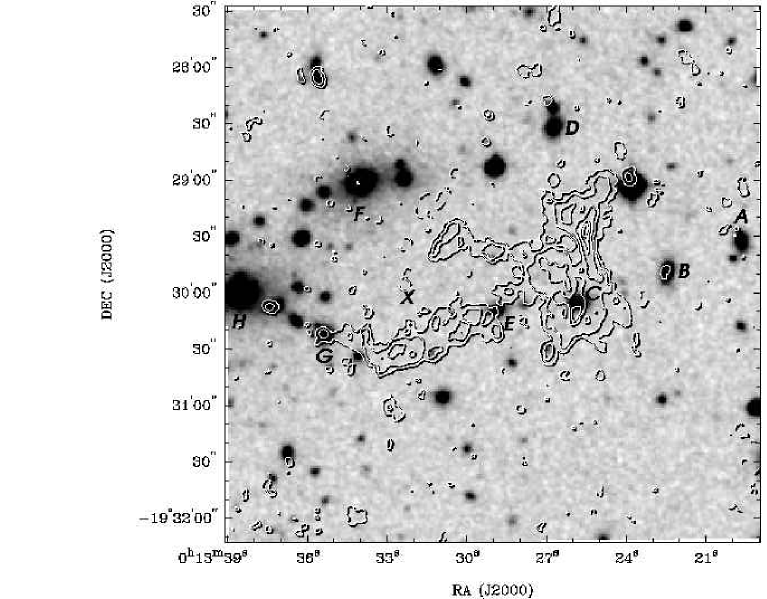
Figure 2: Radio contours of the relic in A13, corresponding to the grey-scale image in Fig. 1, are overlaid on a red DSS-2 image of the area. The contour levels are ($-$43 (dashed), 43, 86, 173, 303, 389) $\mu$Jy beam^-1 or ($-1.47,1.47,2.9,5.8,10.2,13.0$) K. The labelled galaxies are discussed in §3.4.

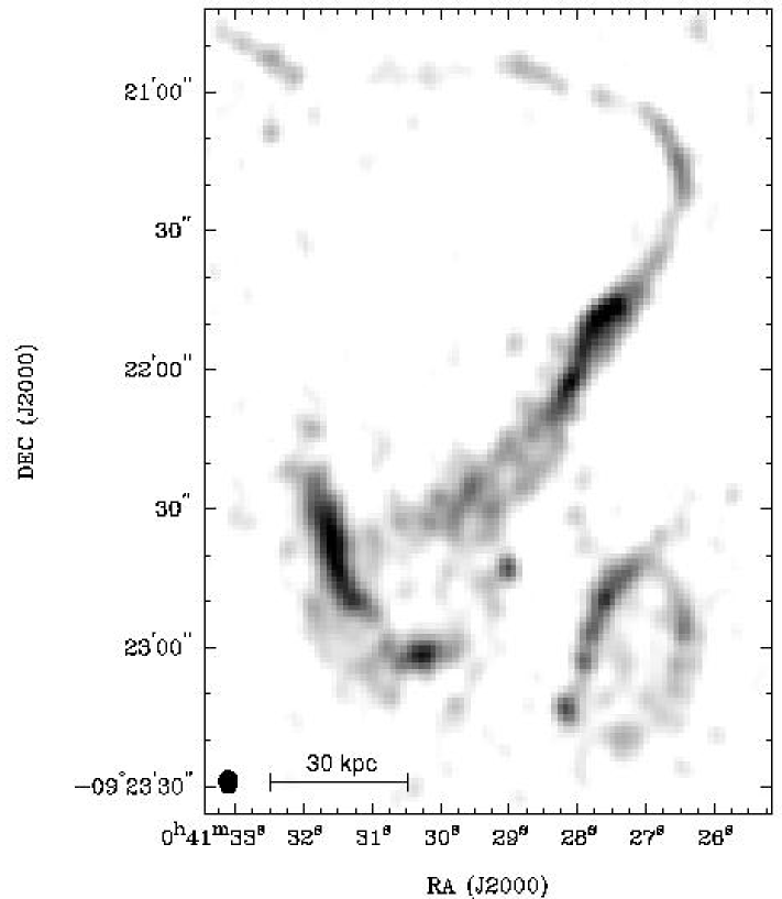
Figure 3: VLA uniformly-weighted image of the relic in A85 at 1.425 GHz. The FWHM restoring beam in the lower left corner is 5.0${}^{\prime\prime}\times 4.2^{\prime\prime}$ in PA = 5^∘. The surface brightness varies from 30 $\mu$Jy beam^-1 to 300 $\mu$Jy beam^-1 (1.3 K to 12.5 K), and the r.m.s. noise level outside the source is 17.4 $\mu$Jy beam^-1 (0.75 K). The horizontal bar indicates the linear scale, using the redshift from Table 1.

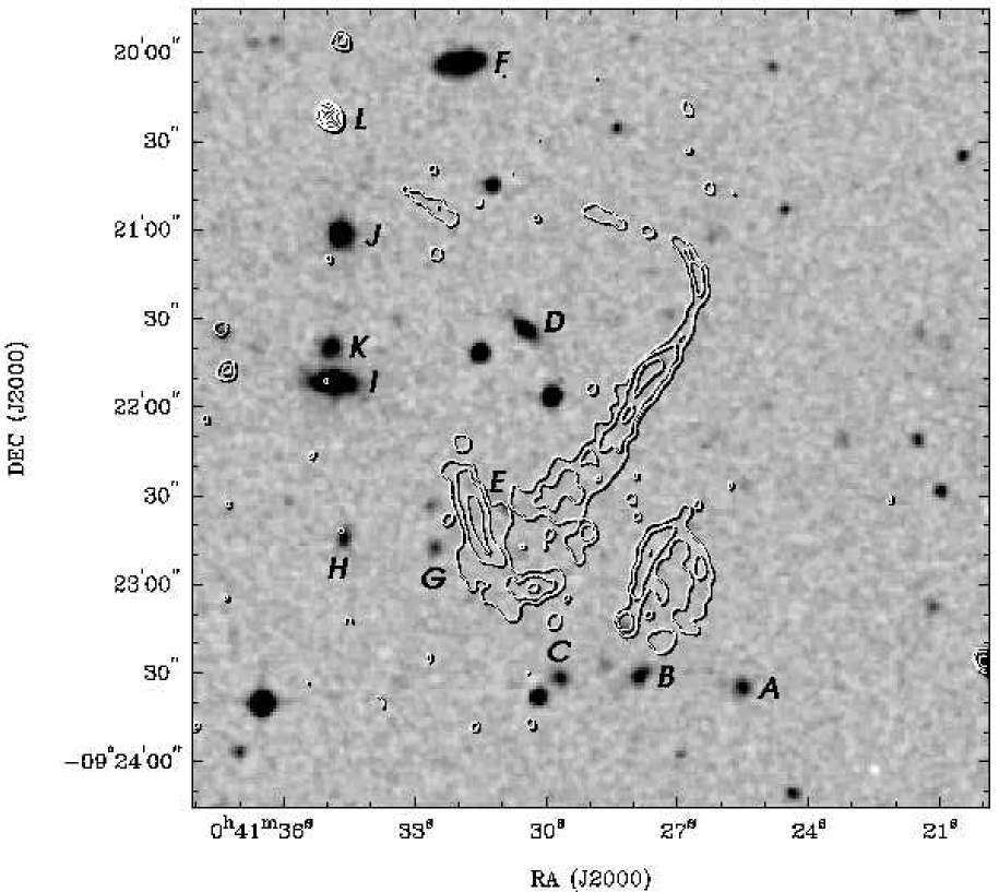
Figure 4: Radio contours of the relic source in A85, corresponding to the image in Fig. 3, are overlaid on a red DSS-2 image of the area. The contour levels are ($-$43 (dashed), 43, 85, 171, 239, 307) $\mu$Jy beam^-1 or $(-1.8,1.8,3.6,7.1,9.9,12.7)$ K. The labelled galaxies are discussed in §3.4.

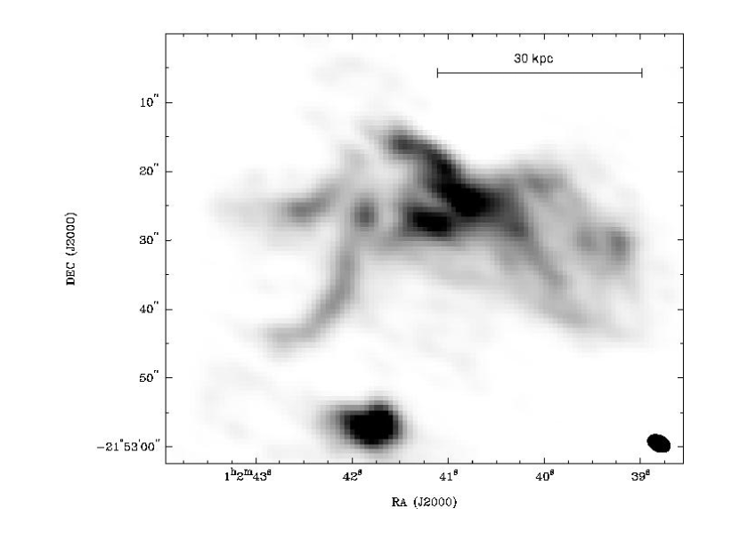
Figure 5: VLA uniformly-weighted image of the relic in A133 at 1.425 GHz. The FWHM restoring beam in the lower right corner is 3.5${}^{\prime\prime}\times 2.4^{\prime\prime}$ in PA = 64^∘. The compact image at the bottom is the source identified with the cD galaxy at the cluster centroid. The surface brightness varies from 25 $\mu$Jy beam^-1 to 3000 $\mu$Jy beam^-1 (2.6 K to 310 K) and the r.m.s. noise level outside the source is 21.1 $\mu$Jy beam^-1 (2.21 K). The horizontal bar indicates the linear scale, using the redshift from Table 1.

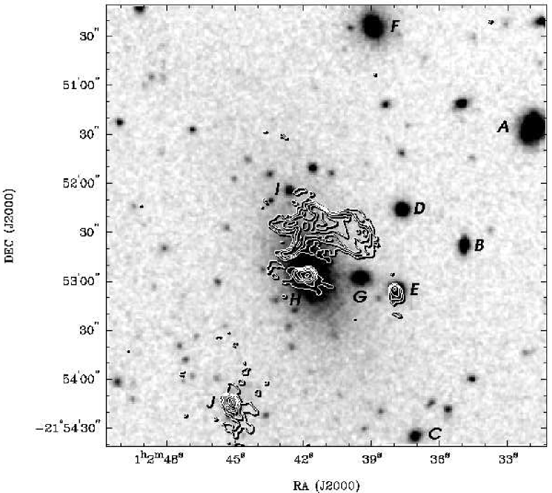
Figure 6: Radio contours of the relic source in A133, corresponding to the image in Fig. 5, are overlaid on a red DSS-2 image of the area. The contour levels are ($-$95 (dashed), 95, 237, 475, 950, 2137, 3325, 4275) $\mu$Jy beam^-1 or $(-9.9,9.9,24.5,49.1,98.2,221,344,442)$ K. The labelled galaxies are discussed in §3.4.

Figs. 1, 3, and 5 show the relics in A13, A85 and A133, respectively. Figs. 2, 4, and 6 overlay the radio images on red images from the Digitized Sky Survey (DSS-2). The corresponding images of A4038 are shown by Slee & Roy (1998). The relics show a remarkable variety of fine structure that takes the form of arcs, filaments and loops of enhanced surface brightness. Most of the arcs and filaments are barely resolved (5 kpc) in their transverse directions, but can have projected lengths of up to 100 kpc. The largest projected linear size of the relics (assuming that they lie within the clusters) varies from 55 kpc (in A133 and A4038) to 260 kpc (in A13). There is no consistent morphology among the relics; in A133 (Fig. 5), four arc-like features appear to radiate from the high-brightness centre of the relic, and in A13 and A85 the structures have various orientations. The arcs and loop in A85, for example, undergo large changes in direction, the loop in the south-west structure showing a reversal of $\sim$ 180^∘. The relic in A4038 (Slee & Roy 1998) has a morphology that is most similar to that of A85.

The A85 relic has been imaged by Giovannini & Feretti (2000) at 333 MHz with 20^′′ resolution. Their image shows low-brightness extensions to the north-east (NE) and south-east (SE) of our 1.425 GHz image, although a conspicuous void is centred south of galaxy $D$ in our Fig. 4. Galaxy $J$ lies within the tip of the NE extension. Our high-resolution image shows some contribution from the NE extension, and also from the SE extension when we lower the grey-scale image to the 2 $\sigma$ level rather than the 3 $\sigma$ level of Fig. 3.

We compute from Giovannini and Feretti’s average surface brightness of about 20 mJy beam^-1 at 333 MHz that we would not have detected these extensions at the 3 $\sigma$ level if the spectral index of this diffuse radiation were $\geq$ 2.1. Since they measure a spectral index over the whole relic of $\alpha$ = 2.5 to 3.0, which is steeper than this limit, we do not expect to detect the extensions seen in their image because it will be below our brightness sensitivity. Thus, it is not necessary to invoke a lack of low spatial frequencies in our high-resolution image to explain the apparent absence of the diffuse emission in Fig. 3.

The extensions are also seen at poorer resolution in the 1.4 GHz image from the NRAO-VLA Sky Survey (NVSS, Condon et al. 1998), which has better brightness sensitivity than our high-resolution image. This diffuse emission must still be contributing to our measured flux density in Table 2, which shows that there is no significant deficit in our value with respect to NVSS.

Rizza et al. (2000) suggest that their less-sensitive, lower-resolution VLA image of the relic in A133 shows a narrow bridge of emission between the cD and the relic with brightness $\sim$ 1 mJy beam^-1 at 1.4 GHz. They interpret this as a perturbed jet propagating through a cooling flow, giving rise to an amorphous radio lobe. Our image (Fig. 5) does not support the presence of this jet. The average 1.425 GHz brightness in the gap between the south-east filament (which itself is curving away from the cD) and the cD is only 26 $\mu$Jy beam^-1, not far above the rms noise level in regions well away from radio sources. When we convolved our image with Rizza et al’s beam, there was still no convincing connection of the form that is shown in their image.

The referee suggests that the relic in A133 might actually be the lobe of a normal radio galaxy whose jet is approaching us at a small angle to the line of sight, and that the counterlobe lies in the south-east part of the NVSS image. However, the suggested counterlobe in the SE of the NVSS image is predominantly due to the source identified with galaxy $J$ in Fig. 6. The relic and the source coincident with the cD could be the approaching and counter lobes of a radio galaxy (with the cD as the host), provided one is prepared to accept that both lobes possess unusually steep spectra (spectral indices of 2.1 in Table 2), and that the lobes differ by a factor of $\simeq 6$ in flux density and linear size. Since other cluster radio galaxies do not possess such extreme differences in lobe parameters (Slee et al. 1998, Table 2), we propose that the relic is not the lobe of a conventional radio galaxy that is associated with the cD. The referee further suggests then that the relic could be a wide-angle tail radio galaxy seen close to side-on and so is seen with the tails projected onto each other, although again the observed spectral index is unusually steep for a conventional radio galaxy. One might be able to test this proposal observationally since the relatively long lines of sight through the radio-emitting plasma should produce a large Faraday depolarization.

3.2 The Flux Densities and Radio Spectra

3.2.1 The High-Resolution Images

We measured the integrated flux density within a rectangular box surrounding each relic and, to estimate the uncertainties due to thermal noise and residual sidelobes of incompletely cleaned field sources, we executed the process 11 times, varying the box sizes and locations around the relic centroids. Systematic errors were estimated to be 3 % for the flux-density scale, 1 % for the flux-density bootstrapping and 3 % for the deconvolution, estimated by repeated deconvolution with various values of the deconvolution control parameters. When added in quadrature, the total uncertainty on our flux-density measurements was 4.5 % to 5.0 %, and the resulting flux densities are given in Table 2.

To estimate the integrated spectral index, we measured the integrated flux density over the relic 11 times at 1.385 GHz and 1.465 GHz within a rectangular box that was varied in area by a factor of four and with box centers that were offset in the E-W and N-S directions from the relic centroid, but always included the whole of the relic. From each pair of measurements we derived the spectral index. Thus we made 11 experimental observations of a constant value, and the measurements differ slightly from each other due to differing contributions of thermal noise, and sidelobes, depending on the box size. Systematic errors are virtually identical at both frequencies. From the 11 measurements we determined the sample mean. The precision of the sample mean was estimated by the standard error of the mean. The integrated spectral indices at the central frequency of 1.425 GHz were in the range 2.1 to 4.4.

We estimated the potential missing flux density due to resolution effects by measuring flux densities from the images in the NVSS. The survey has a beamwidth of $45^{\prime\prime}$ and so suffers less from missing flux density but suffers more from confusion with nearby unrelated sources. We measured flux densities from the NVSS images in the same manner as explained above, but then subtracted the contributions of unrelated sources that are clearly seen and measurable in our higher-resolution images. These 1.40 GHz flux densities from the NVSS are listed in Table 3 and are discussed further in §3.2.2. The flux density missed from each relic by our present high-resolution observations was computed by subtracting the flux-density measurement at high resolution (Table 2; corrected for the frequency difference) from the flux-density measurement from the NVSS, and the largest difference amounted to 17 % of the corrected NVSS flux density. The flux-density differences are given in Table 2. The uncertainties in these values are large because they are small differences between large quantities. Our flux-density estimates are not significantly lower than those of the NVSS.

We attempted to measure the variation in spectral index over each relic, but found when we subdivided the relic, the signal-to-noise ratio dropped to such an extent that, with a frequency base of only 80 MHz, the uncertainty on the spectral indices was too large for the spectral index measurements to be useful.

3.2.2 The Integrated Spectra

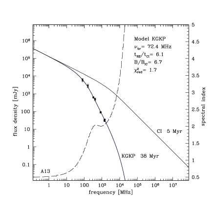
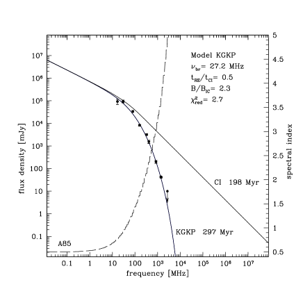
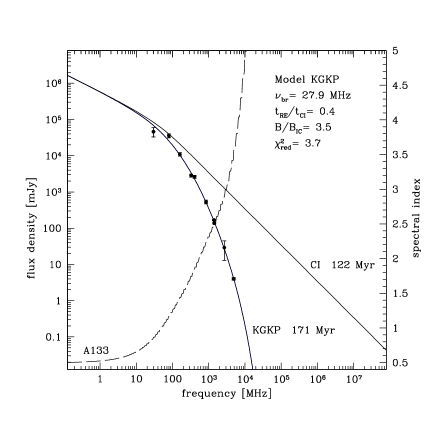
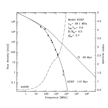
Figure 8: KGKP model fits to the spectra of four relic sources, based on spectral data from Table 3. The Abell name is indicated in the lower-left corner of each panel. The continuous lines are the best-fitting spectra from the KGKP model and expected CI spectrum at the cessation of injection (left-hand axis); the dashed line is the KGKP model spectral index (right-hand axis). Along with the model names, the CI phase duration and the total source age are indicated.

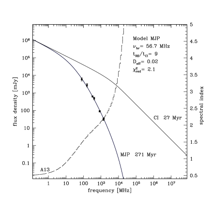
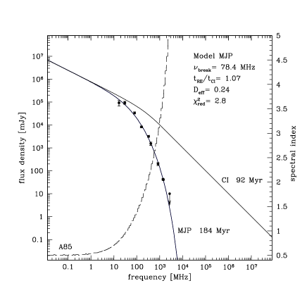
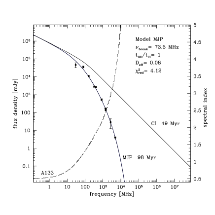
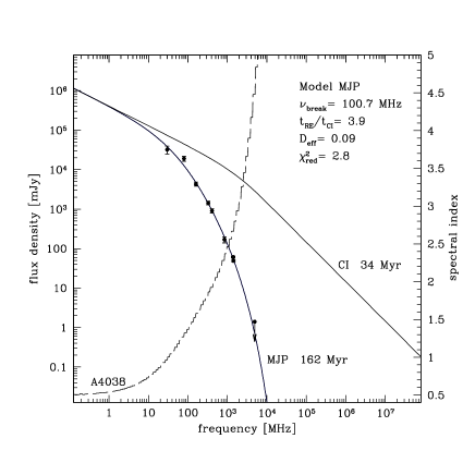
Figure 9: MJP model fits to the spectra of four relic sources, based on spectral data from Table 3. The Abell name is indicated in the lower-left corner of each panel. The continuous lines are the best-fitting spectra from the MJP model and expected CI spectrum at the cessation of injection (left-hand axis); the dashed line is the MJP model spectral index (right-hand axis). Along with the model names, the CI phase duration and the total source age are indicated.

Additional flux-density measurements at other frequencies from the literature were used to plot the broad-band spectra of the relics in Figs. 8 and 9, using the data in Table 3. The details of these measurements are given in the following notes, which are numbered in column 10 of Table 3.

(1) The 16.7 MHz measurements were made by Braude et al. (1981) with a FWHM beam of 40${}^{\prime}\times$80^′. The excess flux density included in their value (column 3) from the many other sources within their beam was estimated by summing the flux densities from the 1.4 GHz sources in NVSS that fell within this beam and extrapolating that value to 16.7 MHz with an assumed average spectral index of 0.80 $\pm$ 0.1; the error in the excess flux density reflects the range of assumed spectral indices. Braude et al. made an absolute calibration of their flux-density scale, which is close to the extrapolated scale of “KPW” (Kellermann, Pauliny-Toth & Williams 1969). The authors give a flux-density error that includes the effects of noise and confusion, although they could not have included the contributions of the many sources within their beam, as we have outlined above.

(2) The 29.9 MHz measurements of Finlay & Jones (1973) were made with a FWHM beam of 50${}^{\prime}\times$50^′ at the zenith. The corrections for the excess flux densities of the numerous sources within their beam (columns 3, 5, 7) were made as explained above. The authors made an absolute calibration of their flux-density scale, which they found was $\sim$ 5 % above the extrapolated KPW scale.

(3) The 80 MHz measurements of Slee (1995) were made with a FWHM beam of 3.75^′ at the zenith. The only correction for confusion necessary was for the source A133_8 (Slee et al. 1994, present paper), which has a well-determined spectrum. The flux-density scale was that of KPW and the random errors (Slee & Higgins 1973) depend on the flux density and number of measurements contributing to the average. The total error varied between 12 % and 20 %, including a contribution of 10 % for uncertainty in the flux-density scale.

(4) The 160 MHz measurements of Slee (1995) were made with a FWHM beam of 1.85^′ at the zenith. No corrections for confusion were necessary. The flux-density scale was that of KPW and the errors are discussed in Slee (1977).

(5) The 408 MHz measurements of Reynolds (1986) and Slee & Reynolds (1984) were made with a FWHM beam of 2.6${}^{\prime}\times$2.9^′ at the zenith. Small corrections for confusion were needed for A133_8, and A4038_10, A4038_11 (Slee et al. 1994) using a flux density extrapolated from 1.5 GHz. An absolute calibration of the 408 MHz flux-density scale was made by Wyllie (1969), and Reynolds (1986) suggests that errors of $\sim$ 15 % are appropriate for these flux densities.

(6) The 843 MHz measurements of Reynolds (1986) and Slee and Reynolds (1984) were made with a FWHM beam of $40^{\prime\prime}\times 40^{\prime\prime}$ cosec($\delta$). Corrections for confusion were necessary only for A4038_10 and A4038_11 (Slee et al. 1994) using the extrapolated flux densities from 1.5 GHz. Reynolds (1986) suggests that errors of $\sim$ 7 % are appropriate.

(7) The 1.4 GHz flux densities from NVSS (Table 3) were used rather than our measured values from Table 2, to include any flux density that our high-resolution measurements may have failed to detect. The NVSS FWHM beam of 45^′′ includes the sources A133_8, A4038_10, A4038_11; we have corrected the NVSS total flux densities by subtracting the VLA flux densities given in Table 2 for those sources. The NVSS flux-density scale is that of Baars et al. (1977) and has an error of 3 % to 4 %, and the combined error is unlikely to exceed 5 % to 10 %, depending on the flux density.

(8) The 2.7 GHz measurements of Andernach et al. (1986) and Reuter & Andernach (1990) were made with a FWHM pencil beam of 4.4^′. A substantial correction was made for A133_8 by extrapolating from our present 1.425 GHz flux using the known spectral index from Slee et al. (1994). The flux-density scale is that of Baars et al. (1977) and the total error quoted by the authors for the relic in A133 was 30 %.

(9) The 4.9 GHz measurement of the relic in A133 from Slee et al. (1994) was made with the VLA with a FWHM beam of 21${}^{\prime\prime}\times$14^′′. No corrections for confusion were needed. The flux-density scale was that of Baars et al. (1977) and the total error was 7.5 %. The upper limit for A4038 was based on multiplying the 3 $\sigma$ brightness limit by the number of beam areas subtended by the source.

We believe that the flux densities in Table 3 are free of errors associated with the inclusion of field sources within the beam of the low-resolution telescopes, and that the quoted errors include the uncertainties in the flux scales adopted by various observers.

The broad-band spectra in Figs. 8 and 9 show a characteristic curvature with pronounced flattening at the low-frequency end; at frequencies below $\sim$ 100 MHz the slopes of the spectra are flatter than $\alpha$ = +1, whilst near 1.425 GHz the spectra are much steeper with spectral indices given in Table 2. The significance of the high degree of curvature seen in these spectra will be explored using spectral-ageing models developed in §5.

As a consistency check, we compared the spectral index at 1.425 GHz from the broad-band spectra to the spectral index at 1.425 GHz from the high-resolution images, using model fits to the broad-band spectra from §5 to interpolate between the data points of the broad-band spectrum taking into account the spectral curvature over a broad frequency range. We found serious discrepancy only for A13. Details of the comparison are in §5.4.

3.3 Polarization

When estimating the average polarization fraction, we subdivided each relic into between ten and 16 approximately equal regions, each containing about 20 beam areas. The polarized flux density and total intensity were measured for each region, resulting in ten to 16 values for the polarized fraction. The average polarization fraction over each relic was determined using the sample mean. The polarization fraction varies systematically within the relics by an amount that is large compared to the random noise in the image and so, in contrast to the case of the spectral index measurement, the sample standard deviation quantifies an interesting property of the relics, that is, how much the polarization fraction differs from the mean from region to region. We quantify this variation by using the standard deviation. The average polarization percentages with their standard deviations are listed in Table 2. The position angle of the electric vector at the source is not known for any of these relics because we lack the higher-frequency image with similar angular resolution with which to determine the rotation measure.

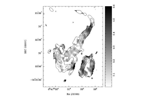
Figure 10: Radio contours from the naturally-weighted image of the A85 relic are overlaid on the naturally-weighted grey-scale image of fractional polarization at 1.425 GHz. Pixels are blanked when the polarized flux is $\leq$ four times the r.m.s. noise level. The polarized fraction is given by the vertical scale on the right-hand side. The radio contours are at (92, 185, 369, 738) $\mu$Jy beam^-1 or $(3.1,6.2,12.4,24.7$) K.

The high value of the standard deviation of the polarization fraction in A85 reflects a significant variation in different parts of the relic. Figure 10 shows that the polarization varies between $\sim$ 35 % in the north-west area, $\sim$ 25 % in the south-west loop and 5 % to 10 % in the south-eastern arc. There is no clear correlation between polarization and total intensity. Unfortunately, the lack of comparable accuracy in the measurement of spectral index prevents our searching for a relationship between polarized fraction and spectral index.

The polarization varies significantly among these three relics. A85 is highly polarized in some areas at 1.425 GHz, implying that the fields are not highly tangled and that Faraday depolarization is low. Conversely, A133 and A4038 have low fractional polarization. Whether this is due to tangled fields and/or Faraday depolarization can be determined only when a higher-frequency image of similar angular resolution becomes available.

3.4 Optical Identifications

The identification of galaxies with which these relics may be associated is an uncertain pursuit, but one can make some progress. First, if the relics are the remnants of conventional radio galaxies, then the former host should be a bright elliptical with $M_{\mathrm{R}}\leq-21.0$ (cf. Ledlow & Owen 1995; Slee, Roy, & Andernach 1998). Second, the galaxy should be close enough to the relic that it could have moved to its present distance in the lifetime of the relic. The brightest cluster member (BCG) is naturally the prime suspect, provided that it satisfies the distance criterion. Note, however, that these travel-time arguments are uncertain because of the use of projected spacings and velocities, which vary respectively as the cosine and sine of the angle with respect to the plane of the sky. The distance criterion can also be affected strongly by intracluster winds, which are known to shape the tails of many tailed sources in clusters and which might exceed 1000 km s^-1 (Burns 1998). Such a wind could carry a relic away from the host faster or slower than expected from the peculiar motion of the host galaxy, depending on the vector addition of wind and host velocities. We have, unfortunately, no knowledge of wind speeds or directions in any of these four clusters, and so the travel times we derive are probably rather uncertain. The identification should also allow for displacements between the host galaxy and radio centroid that are commonly seen in radio galaxies in clusters. For example, the median differences in projected positions between the radio centroid and optical host in the cluster sample of Slee et al. (1994, 1996) yields medians of 5” for 25 doubles, 13” for seven wide-angle-tail sources and 13” for 13 narrow-angle-tail sources, at an angular resolution of 14”.

A13 - The galaxies identified in Fig. 2 have redshifts compatible with membership of A13 and satisfy the luminosity criterion for a former host galaxy, except galaxy $E$ for which we have no redshift measurement. Travel times for these galaxies from the centroid of the radio relic (10^′′ NW of galaxy E) range from $0.58\times 10^{8}$ yr (galaxy $C$) to $6.6\times 10^{8}$ yr (galaxy $B$), assuming that the velocity vector is at $45^{\circ}$ to the plane of the sky. Only galaxy $C$ has a travel time that is within a factor of two of the relic’s age of $t_{\rm RE}=0.33\times 10^{8}$ yr from the KGKP model of §5; the remaining galaxies have travel times $\geq 1.1\times 10^{8}$ yr, which are better matched by the relic age derived using the MJP model ($t_{\rm RE}\geq 2.44\times 10^{8}$ yr). However, the differences between relic ages from the KGKP and MJP models make it difficult to use the travel times alone to select one of the bright galaxies as a former host.

One could argue that galaxy $C$ is the active host to a source reminiscent of wide-angle-tail radio galaxy with tails stretching to the north and north-east. If so, then the linear structure stretching to the east-south-east could equally well be interpreted as another tailed radio galaxy with active host either galaxy $E$ or $G$ (though it is not certain that $E$ is in A13). However, the extreme spectral indices of both radio structures ($\simeq 4.4$) make it very unlikely that these are active radio galaxies.

The BCGs ($F$ and $H$) are the preferred hosts because optically luminous galaxies are the most likely hosts to radio galaxies (eg Slee et al. 1998, Fig. 18), and the travel times ($1.7\times 10^{8}$ yr and $1.2\times 10^{8}$ yr respectively) lie within the range of relic ages estimated by the KGKP model ($t_{\rm RE}=0.33\times 10^{8}$ yr) and the MJP model ($t_{\rm RE}\geq 2.44\times 10^{8}$ yr).

A85 – The BCG (a cD) lies 395 kpc to the north-east of the relic’s centroid and is well outside the optical overlay in Fig. 4. Its low peculiar velocity ($\leq$ 100 km s^-1) results in a travel time from the relic of $\geq$ 4$\times$10⁹ yr (assuming that the velocity vector is at $45^{\circ}$ to the plane of the sky), which would make the relic unreasonably old, unless the relic is due to recompression (Enßlin & Gopal-Krishna 2001).

The brighter galaxies within 2.5^′ (160 kpc) of the relic’s centroid are labelled in Fig. 4. All have measured redshifts that place them in the cluster, except galaxies $I$ and $F$ which are foreground and have recession velocities that differ from the cluster velocity by two and a half and three times the cluster velocity dispersion, and galaxies $C$, $E$, and $G$ for which no redshifts have been measured. Of the galaxies known to be in the cluster, only $J$ barely fulfils the luminosity criterion for a radio galaxy, having $M_{\mathrm{R}}=-21.0\pm 0.2$. It lies near the north-eastern tip of a low-brightness extension of the relic, which is more clearly detected in the 333 MHz image of Giovaninni & Feretti (2000) than in our high-resolution images. (However, note that the 333 MHz image confuses the compact radio source marked $L$ in Fig. 4 with the relic.) If $J$ is the former host, its projected distance from the relic centroid (128 kpc) and its peculiar radial velocity (676 km s^-1) yield a travel time from the relic of 1.8$\times$10⁸ yr, which is within a factor of two of the spectral age ($1.0\times 10^{8}$ yr) derived for the relic in §5.

We conclude that if the relic was a radio galaxy and a member of A85, then its former host is most likely to be galaxy $J$, which is still embedded in a diffuse relativistic plasma visible at 333 MHz.

A133 – the brighter galaxies within 2.5^′ of the relic’s centroid are labelled in Fig 6. The galaxies $B,C,E,F,G,H,$ and $I$ possess measured redshifts and those are consistent with cluster membership. Galaxy $J$ is identified with a radio source (A133_8 in Slee et al. 1994) and has a redshift of 0.2930, which places the galaxy well behind the cluster. This source is of interest because it is not properly resolved (if at all) from the relic and the cD in the lower-resolution observations and its contribution has been subtracted in Table 3.

Galaxy $H$ (the cD ) would normally be favoured as the former host, but the travel time to its present position of $1.5\times 10^{8}$ yr (assuming that the velocity vector is at $45^{\circ}$ to the plane of the sky) is three times the relic’s age of $t_{\rm RE}=4.9\times 10^{7}$ yr (§5). The remaining five ellipticals in Fig. 6 that have measured cluster redshifts and are bright enough to qualify as host galaxies ($B,C,E,F,$ and $G$) possess travel times that range from $4.2\times 10^{7}$ yr (galaxy $G$) to $1.6\times 10^{9}$ yr (galaxy $E$). The travel time of galaxy $G$ most closely matches the age of the relic.

In summary, the cD is unlikely to be an active host to a radio galaxy, of which the relic forms one lobe, but it could be the former host, provided one is prepared to accept that the calculated travel time and/or relic age have rather large uncertainties.

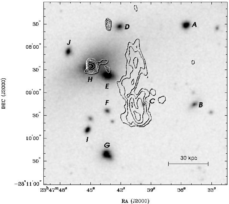
Figure 7: Radio contours of a naturally-weighted image of the relic source in A4038 are overlaid on a red DSS-2 image of the area. The contour levels are (128, 256, 642, 1284) $\mu$Jy beam^-1 or $(4.1,8.1,20.3,40.5)$ K. The FWHM restoring beam for the radio image is $6.9^{\prime\prime}\times 4.0^{\prime\prime}$ in PA$\,=\,2^{\circ}$. The labelled galaxies are discussed in §3.4. The horizontal bar indicates the linear scale, using the redshift from Table 1.

A4038 – The brighter galaxies within 4${}^{\prime}\times$4^′ of the relic’s centroid are labelled in Fig. 7. The galaxies $A,B,D,E,F,G,H,I,$ and $J$ have measured redshifts that are consistent with cluster membership. The image marked $C$ is stellar. The galaxies $A,D,E,G,H,$ and $J$ satisfy the luminosity criterion for a radio galaxy host. The cD (galaxy $H$) is the most likely candidate due to its large luminosity. It is currently host to a radio galaxy, and so if it produced the relic, it is now undergoing a second stage of activity. If the velocity vector lies at $45^{\circ}$ to the plane of the sky, it would have reached its present position from the relic centroid in $3.1\times 10^{8}$ yr. Travel times for the remaining five cluster galaxies range from $4.5\times 10^{7}$ yr to $5.5\times 10^{8}$ yr. Galaxies A,E,G and J have travel times within a factor of two of the relic ages $t_{\rm RE}$ deduced from the spectral modeling in §5, but galaxies D and H (cD) exceed the model ages by factors of at least three to five.

4 Relics and X-ray Emission

Since the pressure of the hot intra-cluster gas is likely to play a significant role in the evolution of cluster relics, it is important to compare the morphologies of radio and X-ray images to search for enhanced X-ray emission from the regions of the relics.

A connection between magnetic fields, cosmic-ray electrons and the cluster X-ray emission recently received further observational support when both Rephaeli, Gruber & Blanco (1999) and Fusco-Femiano et al. (1999) independently reported the discovery of an additional hard X-ray component in the Coma cluster emission with the Rossi X-ray Timing Explorer and BeppoSAX, respectively. Although there is some confusion from the presence of the Seyfert 1 galaxy (X Comae) in the wide field of view of their instruments, both groups find evidence for non-thermal inverse-Compton X-ray emission as predicted for clusters with extended radio sources (Rephaeli 1979). More recently, Enßlin et al. (1999), Dogiel (2000), and Liang (2001) find that the high-energy excess is not likely to be inverse-Compton emission but rather is bremsstrahlung from a non-thermal tail of the electron energy distribution. However, Petrosian (2001) disagrees and concludes that the background thermal electrons cannot be the source of the non-thermal electrons, except for a short period of less than $10^{8}$ yr.

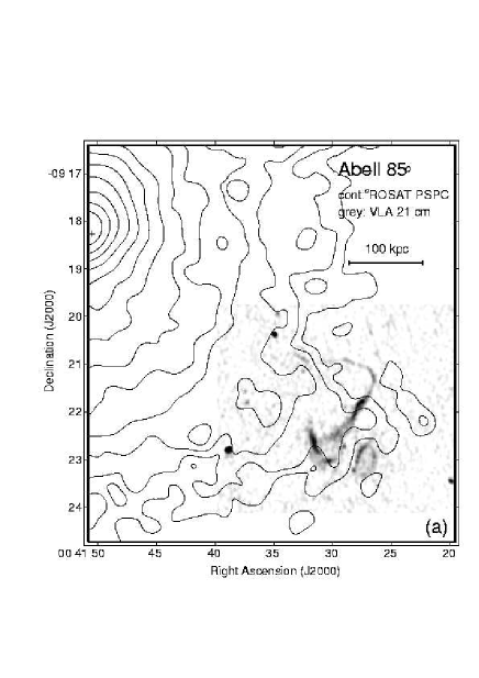
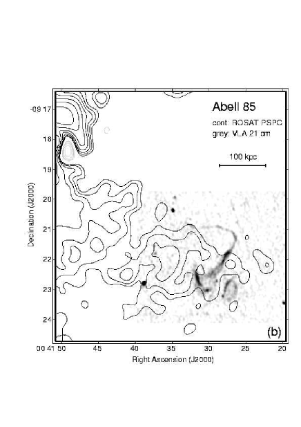
Figure 11: South-western part of A85: (a) ROSAT PSPC hard-band (0.5 keV to 2.0 keV) contours and VLA 1.4 GHz radio image from Fig. 3 as grey-scale. X-ray contours are at $(5,7.07,10,14.1,20,28.3,40,56,80,113,160,226,320)\times 10^{-3}$ count s^-1 arcmin^-2 and the peak is at $447\times 10^{-3}$ count s^-1 arcmin^-2. The resolution of the X-ray map is about 27″ FWHM. The position of the cD galaxy, at top left, is marked by a cross, and the horizontal bar indicates the linear scale, based on the redshift from Table 1. (b) As for (a) but after subtracting a circularly-symmetric three-component Gaussian model from the cluster X-ray emission to remove the cluster thermal emission and improve contrast in regions of excess X-ray emission. X-ray contours are at $(-14.1,-10,-7.07,-5,5,7.07,10,14.1,20,28.3,40)\times 10^{-3}$ count s^-1 arcmin^-2 with negative contours shown in grey and the peak is at $52.8\times 10^{-3}$ count s^-1 arcmin^-2.

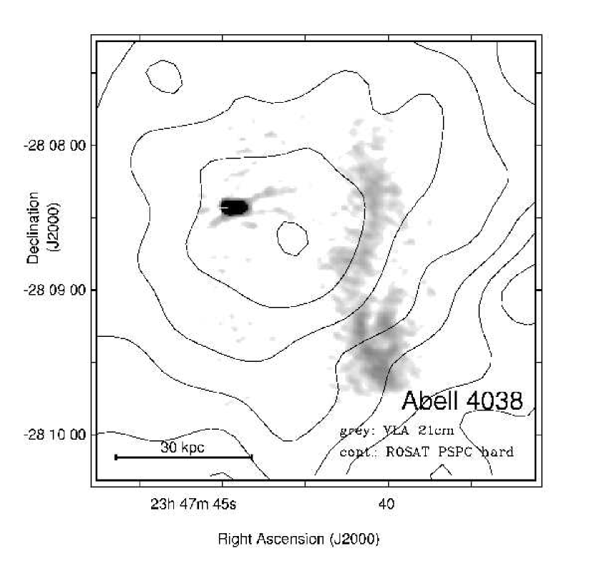
Figure 13: Inner part of A4038: ROSAT PSPC hard-band (0.5 keV to 2.0 keV) contours and VLA 1.4 GHz radio image (cf. Slee & Roy 1998) as grey-scale. X-ray contours are at (5.7, 8, 16, 22.6, 32, and $45.3)\times 3.5\cdot 10^{-3}$ count s^-1 arcmin^-2. The resolution of the X-ray map is about 27″ FWHM. The position of the cD galaxy is marked by a cross and coincides with the eastern end of the compact radio source. The horizontal bar indicates the linear scale, based on the redshift from Table 1.

Pointed X-ray observations are available in the ROSAT archive for A85, A133 and A4038, but for A13 we have only the XBACs data of Ebeling et al. (1996), based on the ROSAT All-Sky Survey (RASS). Our X-ray analysis was performed using the EXtended Scientific Analysis System EXSAS (Zimmermann et al. 1994). Several observations were merged resulting in 15.9 ks PSPC and 31.7 ks HRI exposures for A85 and A133, respectively. In the case of A4038 a single 3.3 ks PSPC data set was available. Binning the PSPC data to a pixel size of 5^′′, we produced images of the central part of the detector window out to 20^′ from the optical axis. These were exposure corrected and an energy-dependent Gaussian filter was applied to compute X-ray color images in the broad (0.1 keV to 2.4 keV), soft (0.1 keV to 0.4 keV) and hard (0.5 keV to 2.0 keV) ROSAT energy bands. Details of the image production are given in Ehle et al. (1998). The PSPC hard-band images of A85 and A4038 are shown as contour plots overlaid on grey-scale radio images of the relic sources in Figs. 11a and 13, respectively.

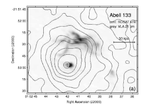
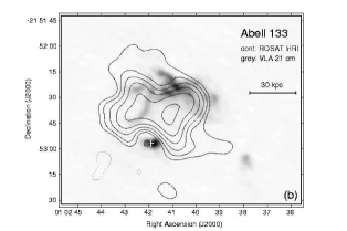
Figure 12: Inner part of A133: (a) ROSAT HRI (0.1 keV to 2.4 keV) contours and VLA 1.4 GHz radio image from Fig. 5 as grey-scale. X-ray contours are at (0.008, 0.011, 0.016, 0.023, 0.032, 0.045, 0.065, 0.091, 0.128, 0.182) count s^-1 arcmin^-2 and the peak is at 0.193 count s^-1 arcmin^-2. The resolution of the X-ray map is 12″ FWHM. The position of the cD galaxy is marked by a cross, and the horizontal bar indicates the linear scale, based on the redshift from Table 1. (b) As for (a) but after subtracting an azimuthally-averaged image of the cluster X-ray emission to remove the cluster thermal X-ray emission and improve contrast in regions of excess X-ray emission in the region of the relic. X-ray contours are at (-0.008, 0.008, 0.011, 0.016, 0.023, 0.032, 0.045) count s^-1 arcmin^-2 with negative contours shown in grey and the peak is at 0.0495 count s^-1 arcmin^-2.

To minimize the HRI instrument background on A133 (due to UV emission and cosmic rays) without degrading the X-ray sensitivity, we selected raw amplitudes from only channels 2 to 8 for our analysis (see David et al. 1993). The HRI image was constructed with a pixel size of 1^′′ and smoothed with a Gaussian filter of 12^′′ FWHM. The HRI contour map of A133 is overlaid on a grey-scale radio image of the relic source in Fig. 12a.

To improve contrast in regions of excess X-ray emission in the region of the relic, we attempted to subtract the cluster thermal emission component from A85, A133 and A4038. For A85, we achieved the lowest residuals by subtracting a simple circularly-symmetric Gaussian model consisting of three components that had a common centre point, located at the peak of the cluster X-ray emission, and that had differing widths and amplitudes. (The FWHM of the components were 110”, 310”, and 750”, and the relative peak heights were 1.0, 0.168, 0.076.) For A133 we subtracted a mask created by azimuthally-averaging the image of the cluster X-ray emission. The centre of rotation was the peak of the cluster emission, and the lower half-image only was used since we found that including the relic emission in the mask resulted in over-subtraction of the region south of the X-ray peak. For A4038 we tried subtracting various models centered on the X-ray peak, which itself was offset from the cD in the direction of the relic. No convincing feature in the residual image was associated with the relic. The resulting residual images for A85 and A133 are shown in Figs. 11b and 12b.

The plots in Figs. 11, 12 and 13 show a slightly enhanced diffuse X-ray emission in the region of the radio source (A85 and A133) or a shift of the X-ray emission centroid towards the relic (A4038). The excess X-ray emission seen in Figs. 11b and 12b is most pronounced in the hard energy band, as can be expected for inverse-Compton emission, which has a flatter spectrum than the cluster’s thermal emission, more in keeping with the radio spectral indices present in the low-frequency parts of Figs. 8 and 9. We note that in the case of A85, enhanced X-ray emission in the relic region was also reported by Bagchi, Pislar & Lima Neto (1998). However, there appears to be a difference between the spectral composition of excess X-ray emission seen in the Coma halo and the present relics. Our relics are associated with excess emission in the energy range 0.5 keV to 2 keV, while the excess in Coma is detected only above 18 keV. This could be explained most easily by a difference in the very-low-frequency spectral indices of halos and relics; relics could have a higher density of relativistic electrons radiating at the lower frequencies that most efficiently scatter CMB photons to our lower energy X-ray spectral band.

The excess X-ray flux from the region of the radio relic, measured from the residual X-ray images is $2.05\times 10^{-12}$ erg cm^-2 s^-1 for A85 and $8.97\times 10^{-13}$ erg cm^-2 s^-1 for A133, estimated for the 0.5 keV to 2.4 keV band and corrected for Galactic H I absorption. Integrating the radio flux from Table 3 between 10 MHz and 100 MHz yields integrated fluxes of $5.10\times 10^{-17}$ W m^-2 for A85 and $3.61\times 10^{-17}$ W m^-2 for A133. Assuming that the X-ray flux is from inverse-Compton scattering, the magnetic field inferred following Bagchi et al. (1998) is 0.47 $\mu$G for A85 and 0.60 $\mu$G for A133. The value for A85 differs by a factor of two from the ($0.95\pm 0.10$) $\mu$G found by Bagchi et al. At least a part of this difference is probably due to differences in the details of calibrating and measuring the X-ray and radio fluxes.

Confirmation of the presence of inverse-Compton emission in radio relics will only come from the present generation of X-ray telescopes such as XMM-Newton and Chandra. These have the angular and spectral resolution to match those of the present radio images, and are sensitive to higher energies than ROSAT, which should provide better contrast between inverse-Compton emission and the cluster thermal emission.

5 Spectral Modelling

The shape of the radio spectrum from 10 MHz to 5 GHz results from the competition between energy injection and losses due to adiabatic expansion, synchrotron emission, and inverse-Compton scattering off cosmic microwave background (CMB) photons, and a detailed understanding of these processes can yield the age of the relic, the duration of initial particle injection, and the magnetic field strength.

5.1 The Komissarov & Gubanov Models

Well-developed models of relic sources have been published by Komissarov & Gubanov (1994); they include a discussion of the relics in A85 and A133 that are presented in this paper. The authors explored the possibility that these extremely steep-spectrum radio sources could be the remnants of powerful radio sources whose nuclei have ceased to produce jets. They assumed a finite duration for the continuous injection (CI) of relativistic electrons, $t_{\rm CI}$, followed by a relic (RE) phase of duration $t_{\rm RE}$ during which the injection of relativistic electrons is switched off. During both the CI and RE phases, the electrons lose energy by synchrotron emission and inverse Compton (IC) scattering off CMB photons. They supposed that the magnetic field in the lobes is uniform and constant and calculated the broad-band synchrotron spectrum by modifying the classical Kardashev-Pacholczyk (KP) model (Kardashev 1962) and the Jaffe-Perola (JP) model (Jaffe & Perola 1973). Both the KP and the JP models consider an isotropic injection of electrons. The KP model describes the situation in which the time-scale for continuous isotropization of the electrons is much longer than the radiative lifetime, each electron maintaining its original pitch angle with respect to the magnetic field. Since the synchrotron losses depend on the magnetic field strength, $B$, and on the pitch angle, $\theta$, as $(B~{}{\rm sin}\,\theta)^{2}$, the small pitch-angle electrons save their energy and the distribution becomes anisotropic.

In contrast, the JP model allows for very efficient pitch angle scattering and the electron distribution stays isotropic. If inverse-Compton losses are taken into account, the energy $\epsilon$ of a single electron evolves at a rate given by

$$\frac{d\epsilon}{dt}=-(b_{\rm syn}+b_{\rm IC})\epsilon^{2}$$ (1)

where factors $b_{\rm syn}$ and $b_{\rm IC}$ describe synchrotron and inverse-Compton losses, respectively. The electron’s synchrotron losses for the KP model and the JP model, are given by

$b_{\rm syn}({\rm KP})=c_{2}B^{2}(\sin^{2}\theta)$

and

$b_{\rm syn}({\rm JP})=c_{2}B^{2}\cdot(2/3)$

where $c_{2}=2.37\cdot 10^{-3}$ erg^-1 s^-1 gauss^-2 is a constant (Pacholczyk 1970). Because of the isotropy of the CMB radiation field, the inverse-Compton-loss term is independent of pitch angle for both the JP and KP models

$b_{\rm IC}({\rm CMB})=c_{2}B_{\rm CMB}^{2}\cdot(2/3)$

$B_{\rm CMB}=3.25\cdot(1+z)^{2}$ ${\rm\mu G}$ (where $z$ is the source redshift) is the magnetic field strength with energy density equal to that of the CMB. Hence, adopting an effective IC magnetic field of $B_{\rm IC}=\sqrt{2/3}\cdot B_{\rm CMB}$, we combine synchrotron and inverse-Compton losses according to

$b_{\rm syn}({\rm KP})+b_{\rm IC}=c_{2}B^{2}(\sin^{2}\theta+B_{\rm IC}^{2}/B^{2})$

$b_{\rm syn}({\rm JP})+b_{\rm IC}=c_{2}B^{2}(2/3+B_{\rm IC}^{2}/B^{2})$.

Here we refer to the anisotropic and to the isotropic Komissarov & Gubanov model as the KGKP and KGJP models, respectively.

The KGKP model is characterized by five free parameters:

• the injection spectral index of the CI phase, $\alpha_{\rm inj}$,

• the total source age, $t=t_{\rm RE}$+$t_{\rm CI}$,

• the relative duration of the relic phase with respect to the CI phase, $t_{\rm RE}$/$t_{\rm CI}$,

• the ratio between the source magnetic field strength and the effective IC magnetic field, $B/B_{\rm IC}$,

• the flux normalization.

In the emission spectrum three break frequencies appear:

$\nu_{\rm br}\propto\frac{B}{(B^{2}+B_{\rm IC}^{2})^{2}}t^{-2}~{}~{},\hskip 14.22636pt\nu_{\rm br}^{\prime}=\nu_{\rm br}\cdot(1+t_{\rm CI}/t_{\rm RE})^{2}$  ,  and    $\nu_{\rm br}^{\prime\prime}\propto\frac{B}{B_{\rm IC}^{4}}t^{-2}~{}~{},$

where $\nu_{\rm br}$ is the break frequency of the first electron population injected at the beginning of the CI phase, and $\nu_{\rm br}^{\prime}$ is the break frequency of the last electron population injected just before the switch-off. The positions of $\nu_{\rm br}$ and $\nu_{\rm br}^{\prime}$ allow one to determine the durations of the CI and RE phases. The third high-frequency break, $\nu_{\rm br}^{\prime\prime}$, is due to the inverse-Compton losses of the small pitch-angle electrons. Since $B_{\rm IC}$ is known, the ratio between $\nu_{\rm br}^{\prime\prime}$ and $\nu_{\rm br}$ allows one to estimate the magnetic field strength directly.

In the emission spectrum, three asymptotic power laws ($S_{\nu}\propto(\nu/\nu_{\circ})^{-\alpha}$) can be identified:

• $\nu\ll\nu_{\rm br}$, the spectral index is $\alpha=\alpha_{\rm inj},$

• $\nu_{\rm br}\ll\nu\ll\nu_{\rm br}^{\prime}$, the spectral index is $\alpha=\alpha_{\rm inj}+0.5,$

• $\nu_{\rm br}^{\prime}\ll\nu\ll\nu_{\rm br}^{\prime\prime}$, the spectral index is $\alpha=4/3\cdot\alpha_{\rm inj}+1.$

For $\nu\gg\nu_{\rm br}^{\prime\prime}$, the spectrum cuts off exponentially. Power law b) quickly disappears after the switch-off ($t_{\rm RE}>0.05\cdot t_{\rm CI}$) and power law c) is seen clearly only if $B>30\,B_{\rm IC}$.

The KGJP model is characterized by four free parameters:

• the injection spectral index of the CI phase, $\alpha_{\rm inj}$,

• the total source age, $t=t_{\rm RE}$+$t_{\rm CI}$,

• the relative duration of the relic phase with respect to the CI phase, $t_{\rm RE}$/$t_{\rm CI}$,

• the flux normalization.

In this case, the isotropy of the electron population does not permit one to measure the source magnetic field. In the emission spectrum only two break frequencies appear:

$\nu_{\rm br}\propto\frac{B}{(2/3\cdot B^{2}+B_{\rm IC}^{2})^{2}}~{}t^{-2}$,   and     $\nu_{\rm br}^{\prime}=\nu_{\rm br}\cdot(1+t_{\rm CI}/t_{\rm RE})^{2}$.

The asymptotic power-law regions are the same as the KGKP model except for power law c) which never appears. For $\nu\gg\nu_{\rm br}^{\prime}$, the spectrum cuts off exponentially. In the limit $B\rightarrow B_{\rm IC}$ (for which inverse- Compton losses are as important as synchrotron losses) any pitch-angle anisotropy is canceled and the KGKP and the KPJP model converge to the same spectral shape.

Komissarov & Gubanov (1994) concluded that the isotropic KGKP model provides a better fit to the data for their relic sample. In this way they were able to estimate the magnetic field strength of the relics by radio observations alone. We have added to the radio spectra of the relics in A13, A85, A133 and A4038, as compiled from the literature, the new flux-density measurements at 1.425 GHz, and we have fitted the KG models using the program Synage++ (Murgia 2001, in preparation). The fitting procedure finds the best free parameters and the confidence regions using a minimum $\chi^{2}$ technique. Following Komissarov & Gubanov, we kept the injection spectral index fixed at 0.5. We confirm that the KGKP is the best model for all the relics, although for A85 both the KGKP and the KGJP models give comparable $\chi^{2}$ values. The best-fit parameters and the physical parameters obtained for the KGKP are summarized in Tables 4 and 5, respectively. The model fits are shown in Fig. 8, along with the CI spectra expected at the end of the active phase (see §5.3). The radiative ages have been calculated according to:

$$t=1060\,\frac{B^{0.5}}{B^{2}+B_{\rm IC}^{2}}((1+z)\cdot\nu_{\rm br})^{-0.5}~{},$$

where the break frequency is expressed in GHz, the magnetic field in $\mu$G and the radiative age in Myr. In the age calculation the magnetic fields resulting from the fits have been used. These are consistent with the magnetic fields derived by the minimum-energy assumption, $B_{\rm me}$, for A85 and A133 and similar values were derived by Komissarov & Gubanov (1994) for the KP model. For the cases of A13 and A4038, $B_{\rm me}$ is weaker by factors of 3.8 and 1.7, respectively.

The minimum-energy magnetic field was calculated using Miley (1980) Eq. (2) and the standard assumptions that the lower and upper cut-off frequencies are 10 MHz and 100 GHz, the ratio of energy in heavy particles to that in the electrons is unity, the filling factor in the emitting regions is unity, the angle between the magnetic field and the line of sight is 90^∘. We assumed the depth of the source, $s$, to be the linear distance corresponding to the FWHM beam diameter, $\sqrt{\theta_{x}\,\theta_{y}}$, where $\theta_{x}$ and $\theta_{y}$ are the major and minor axes of the restoring beam. The spectrum that is integrated by Miley in Eq. (2) is a single power law with spectral index $\alpha$. However, the observed relic spectra are strongly curved and are not well represented by a single power law. Instead, we treated the spectra initially as a series of piece-wise power laws between the spectral measurements in Table 3 and applied Eq. (2) of Miley to integrate the spectrum over each frequency interval. Then, to extrapolate to the full span of 10 MHz to 100 GHz using Eq. (2) of Miley, we found an “equivalent spectral index” that yielded the same result as the piece-wise integration when integrated over the same range of frequencies. For the integration of the spectrum from 10 MHz to 100 GHz this equivalent spectral index was then used in Eq. (2) of Miley, along with $F_{0}/(\theta_{x}\theta_{y})$, where $F_{0}$ is the median surface brightness of the relic at 1.4 GHz. This procedure yielded the minimum-energy magnetic field strengths listed in Tables 5 and 7. The median $B_{\rm me}=8.8$ $\mu$G is significantly lower than that derived by Slee & Reynolds (1984) for six steep-spectrum sources (including the present four relics) of $B_{\rm me}=15.5$ $\mu$G. The difference can be attributed to our weighting of the spectral indices to account for spectral curvature.

5.2 The Diffusion MJP Model

Here, we develop the KG models by including the effects of particle diffusion between regions of different magnetic field strength, to model the effect on the spectra of the filamentary structure.

An important property of the relic spectra is that the high-frequency steepening is less than exponential, which is best fit by the KGKP-based model when one assumes that the magnetic field is uniform and constant, and hence that there is no pitch angle scattering. However, the KGJP model is considered to be more realistic from a physical point of view, since an anisotropic pitch angle distribution (KP) will self-induce Alfvén waves that will scatter the electron in pitch angle (see the discussion by Carilli et al. 1991). Even if this does not occur, the pitch angle will change when the particle moves between regions of different magnetic field strength.

The detailed images of the relics presented in this work show a variety of fine structure in the form of diffuse emission and filaments. If the brightness contrast between these regions is due to a variation of the magnetic field strength then the superposition of different isotropic spectra, with a range of shifted break frequencies, can mimic the behavior of the anisotropic KGKP model. The effect is particularly noticeable for integrated spectra since all the regions of the source are seen together.

Following Tribble (1993), we explore this alternative by supposing that pitch-angle scattering occurs along with diffusion in a spatially variable magnetic field. We approximate the magnetic field strength distribution with a Maxwellian distribution characterized only by its mean value $\langle B\rangle$. The radiative losses suffered by a single electron are a combination of local losses associated with the magnetic field where the electron is radiating now, and global losses associated with the average field seen by the electron during its diffusion and with the inverse-Compton scattering. Following Tribble (1993), we introduce a “diffusion efficiency” $D_{\rm eff}$. The electron energy losses due to synchrotron radiation are proportional to a combination of the local field, $B$, and the average field:

$$D_{\rm eff}\langle B^{2}\rangle+(1-D_{\rm eff})\cdot B^{2}$$ (2)

$D_{\rm eff}$ and $(1-D_{\rm eff})$ are the fractions of a particle’s lifetime that it has spent in the average field $\langle B\rangle$ and in the actual field, $B$, respectively. For simplicity we consider the diffusion efficiency coefficient to be independent of the energy and the age of the electrons. In the extreme case $D_{\rm eff}=0$ (no diffusion) the losses are determined only by the local field. The break frequency of a particular population of electrons with the same age varies as $\nu_{\rm br}\propto B^{-3}$. When we integrate the contributions from all the different field strength regions the sharp JP cut-off is smoothed out and we see a KP-like spectrum. The other extreme corresponds to $D_{\rm eff}=1$ (strong diffusion). In this limit the electron energy spectrum is the same everywhere because the electrons have sampled all the field strengths. The break frequency varies from place to place as $\nu_{\rm br}\propto B^{-1}$. When we integrate the contributions from all the different field strength regions the sharp exponential JP cut-off is only partially dimmed and we still see a JP-like spectrum. Since $B_{\rm IC}$ acts as a global field, in the presence of inverse-Compton losses we can state a lower limit for the diffusion efficiency :

$$D_{\rm eff}\geq\frac{1}{1+\langle B^{2}\rangle/B_{\rm IC}^{2}}$$

This offers the opportunity to put a lower bound on the source magnetic field from the spectral fits.

The MJP model (Murgia 2001, in preparation) extends Tribble’s (1993) analysis to a situation in which:

• there is an injection phase (CI) of particles with a power law energy spectrum and then a switch-off followed by a relic phase,

• the pitch angle distribution is isotropic (JP),

• the magnetic field is inhomogeneous (i.e. it has fine structure),

• particles may diffuse between regions of different magnetic field strength.

There are five free parameters in the MJP model:

• the injection spectral index of the CI phase, $\alpha_{\rm inj}$,

• the total source age, $t=t_{\rm RE}$+$t_{\rm CI}$,

• the relative duration of the relic phase with respect to the CI phase, $t_{\rm RE}$/$t_{\rm CI}$,

• the diffusion efficiency, $D_{\rm eff}$,

• the flux normalization.

The best-fit parameters and the physical parameters obtained for the MJP are summarized in Tables 6 and 7, respectively. The model fits are shown in Fig. 9, along with the CI spectra expected at the end of the active phase (see §5.3). The goodness of the fits obtained for the MJP model is comparable to that of the KGKP for A85 and A4038, and slightly worse for A13 and A133. The limits inferred for the magnetic field strength are consistent with those of the KGKP. The radiative ages from the MJP model have been calculated according to:

$$t=1060\,\frac{\langle B\rangle^{0.5}}{2/3\langle B^{2}\rangle+B_{\rm IC}^{2}}((1+z)\cdot\nu_{br})^{-0.5}~{},$$

where the break frequency is expressed in GHz, the magnetic field in $\mu$G and the radiative age in Myr. We have assumed that $\langle B\rangle$ is the minimum-energy magnetic field ($B_{\rm me}$), since the field is not computed from the MJP model. The lower limits on the mean magnetic field strength obtained from the estimate of the diffusion efficiency are consistent with those estimated from the minimum-energy assumption for A85, A133 and marginally for A4038 also. In the case of A13, $B_{\rm me}$ is a factor of 3.7 weaker with respect to the lower limit estimated from the fit.

5.3 Luminosities of Progenitors

Both the KGKP and MJP models describe a scenario in which adiabatic expansion and/or compression events are neglected, the magnetic field intensity does not evolve, there is no substantial particle reacceleration and the relativistic electrons do not escape from the source. Indeed, only the radiative losses are supposed to influence the shape of the relic’s spectra after the switch-off. Under these assumptions we extrapolated the relics’ spectra back to the end of the continuous injection phase. These are the CI models shown in Figs. 8 and 9. By measuring the difference between the observed flux densities and those predicted for the CI model we have calculated the 1.4 GHz radio power expected for the progenitor sources at the switch-off instant (see Tables 5 and 7). We found that $P_{\mathrm{1.425\,GHz}}$ ranges from $10^{24.4}$ W Hz^-1 to $10^{25.5}$ W Hz^-1 and from $10^{25.1}$ W Hz^-1 to $10^{26.1}$ W Hz^-1 for the KGKP and MPJ model, respectively. The corresponding total luminosities range from 10³⁴ W to 10³⁶ W. These relatively high $P_{\mathrm{1.425\,GHz}}$ values place the progenitors on the boundary between FR I and FR II radio galaxies, and hence among the most luminous 7 % of radio galaxies (e.g. Slee et al. 1998). Therefore, it seems that only the most powerful radio galaxies in clusters have left radio relics that are detectable with the present generation of synthesis radio telescopes and explains the paucity of detected relics.

5.4 Summary of Spectral Modelling Results

We confirmed that the extremely steep spectra of the relics studied in this work are consistent with the scenario in which the injection of fresh electrons in these sources has ceased for a significant fraction of their lifetime. However, the flux-density measurements indicate that the spectral cut-offs are less than exponential. Under the simple hypothesis that the magnetic field in the relics is uniform, we found that the anisotropic KGKP model fits better than the isotropic KGJP model. In contrast, our VLA images show that the structure of the relics is quite inhomogeneous. By fitting the MJP model we demonstrated that an isotropic distribution of electrons can still reproduce the observed spectra if the brightness contrasts are due to variations of the magnetic field strength. The goodness of the MJP fits is comparable to that of the KGKP, although the KGKP is always slightly better.

The most convincing results were found for A85 and A133 because of the good frequency coverage of their integrated spectra. For these two relics, both the value of the magnetic field strength obtained from the KGKP fits and the lower limits obtained from the MJP are fully consistent with the magnetic fields estimated by minimum-energy arguments.

The integrated spectra of A13 and A4038 were not so well defined and did not allow us to constrain all the fit parameters (particularly for A13). In these cases, the estimates of the magnetic field strengths obtained from fits differ significantly from $B_{\rm me}$. The radiative ages derived from the spectral break frequencies range from $0.3\,\times\,10^{8}$ yr to $2.3\,\times\,10^{8}$ yr for the KGKP model and from $1.0\,\times\,10^{8}$ yr to $2.4\,\times\,10^{8}$ yr for the MJP model.

Finally, we compared the model spectral index at 1.4 GHz resulting from the fit with the spectral index measured from our VLA 1.4 GHz images (Table 2). The model spectral indices for A13, A85, A133 and A4038 are 2.1, 3.8, 2.5, and 2.6, and the observed spectral indices are 4.4, 3.0, 2.1, and 3.1 respectively. Both the KGKP and the MJP models predict very similar spectral indices at 1.4 GHz.

The observed spectral indices were underestimated by the models for A13 and A4038, and overestimated for A85. The spectral index of A133 is fairly well predicted. The most serious discrepancy is found for A13, and it is problematic to explain the origin of this mismatch. In fact, independent of any model, the integrated spectrum of A13 between 160 MHz and 1.4 GHz is almost a power law with a spectral index of $\alpha\sim 2$. The sudden steepening of the spectrum measured from the VLA images is difficult to reconcile with the trend of the integrated spectrum at lower frequencies. The discrepancy could be observational or a real effect. The observed spectral index from the high-resolution VLA measurement could be overestimated due to missing flux from a more extended low-brightness component. However, this seems unlikely because Table 2 shows that our flux-density measurement with the B array actually exceeds that of the NVSS with the D array. Maybe we are witnessing the onset of an exponentially steepening spectral index above 1 GHz as predicted by the JP model. The same process is also present to a lesser degree in the relics of A85 and A4038.

6 Discussion

6.1 Relic Origins and Spectral Models

The radio relics observed here show a surprising amount of fine structure at $4^{\prime\prime}$ resolution. This required us to generalize the spectral-ageing models of relics to include the diffusion of particles between regions of non-uniform magnetic field (§5.2), which yielded better success in fitting the relic spectra than did the scenario for the production of halo and edge relics that used reacceleration of seed relativistic electrons by shocks produced during cluster mergers. Although Roettiger, Burns and Stone (1999) had good success modelling the edge relics in A3667 with this latter approach, the reacceleration process cannot reproduce the much more extreme spectral indices nor the fine structure of the relics considered here. Recent work by Enßlin & Gopal-Krishna (2001) models the relic in A85 as a recompressed radio lobe that had previously expanded and cooled adiabatically, and they obtain an equally good fit to the spectra as we achieved. We shall probably be able to distinguish between the competing mechanisms of an ageing relativistic population and ageing combined with recompression, when more accurate spectral and polarization data are available.

The referee noted a similarity between our relics and the tailed radio galaxy in A3556 which has lost its source of fresh relativistic electrons and has the former host galaxy situated near one extremity of the tail (Venturi et al. 1998). This seems reasonable, however we note that the radio structures are rather different and that still needs to be explained. The tailed radio galaxy is predominantly a linear structure whereas the relics that we have imaged are more complex. The SE extension of the relic in A13 looks like a tailed remnant whose host would be galaxy $C$ or $E$ in Fig. 2, but the remainder of the structure is not linked directly to any nearby galaxy. In A85 and A4038, the likely host galaxies are much more distant from the radio structures than in A3556. The spectra of the relics are also different from the A3556 source, all four being much steeper. This can be explained naturally if our relics have aged longer than has the A3556 source. To compare the spectral ages, we have reanalysed the flux-density measurements of A3556 by Venturi et al. (1998) using the KGKP and MJP models and found the best fit with the MJP model. This model infers a mean field strength $<B>\,\simeq\,1.7\,\mu$G, which agrees well with the equipartition field strength of 1.6 $\mu$G calculated by Venturi et al., and it infers a high value for the diffusion efficiency ($D_{\rm eff}=0.75$). Since the spectrum of the A3556 source is not as steep as our relics, the duration of the relic phase in A3556, $t_{\rm RE}$, should be short compared to the active phase, $t_{\rm CI}$. In fact, the model fits found $t_{\rm RE}/t_{\rm CI}=0.1$ using the KGKP model and $t_{\rm RE}/t_{\rm CI}=0.07$ using the MJP model. These values are considerably lower than those found for our relics and confirm the recent formation of the A3556 tail as a relic. The ages found for the A3556 relic were (KGKP model) $t=520$ Myr, $t_{\rm CI}=470$ Myr and $t_{\rm RE}=50$ Myr, and using the MJP model: $t=490$ Myr, $t_{\rm CI}=458$ Myr and $t_{\rm RE}=32$ Myr. The duration age of the relic phase, $t_{\rm RE}$ is comparable to those found for our relics, but more important for the spectral steepening is that the relative value of $t_{\rm RE}/t_{\rm CI}$ is smaller for the A3556 source.

6.2 Optical Identifications

The identification of former host galaxies for our radio relics is problematic (§3.4). The identification of the relics with the BCGs is by no means certain, because of the disagreement between the modelled relic ages and the galaxy travel times. In fact, there is usually at least one other relatively bright galaxy near the relic that provides a closer match between relic age and travel time than does the BCG, and we found that the most likely identification was with those rather than the BCG for two of the four relics.

6.3 Pressure Balance

We can compare the pressure of the relativistic plasma, $p_{\rm r}$, derived from the radio emission to the pressure of the intra-cluster gas, $p_{\rm ic}$, derived from its X-ray properties, and so understand something about the confinement of the relic. We assumed approximate equipartition between field and particle energies in the radio source, and static isothermal pressure due to the intra-cluster gas. There is not enough information in existing X-ray images to determine radial temperature and electron-density profiles for A13, A133 and A4038, and so we have adopted the profiles determined for A85 by Pislar et al. (1997) and assumed that they are the same in A13, A133 and A4038.

The pressure of the relativistic plasma is $\mu_{\rm me}/3$, where $\mu_{\rm me}$, the minimum energy density, was derived from Miley (1980) Eq.(1). The thermal pressure of the intra-cluster gas is $n\,k\,T\,/\,A_{\rm r}$ dyne cm^-2, where $n$ is the electron density in cm^-3, $T$ the temperature in K, $k=$1.38$\times$10^-16 erg K^-1 and $A_{\rm r}$ = 0.62 is the relative atomic mass for a fully ionized gas containing 10 % He by number. The temperature is scaled from $k\,T\,=\,$4 keV (Pislar et al. 1997) for A85, with the assumption that $T$ $\propto$ (velocity dispersion)² (Mazure et al. 1996). The central electron density of each cluster is scaled from that of A85 on the assumption that it is proportional to the square root of the X-ray luminosity. Therefore, this assumes that the clusters have the same core radius and radial variation in electron density as A85. Model No. 2 from Pislar et al. (1997) was then used to evaluate the electron densities, $n$, at the centroid of the relic, and are given in Table 8.

Comparing the relativistic plasma pressure to the thermal pressure of the intra-cluster gas, we find that pressure equilibrium exists only for the relic in A85. In the remaining three relics, the pressure of the thermal gas is three to five times that of the relativistic plasma. However, the value of $B_{\mathrm{me}}$ in Table 8 could well be increased enough by relatively small departures in the assumptions used to calculate $B_{\mathrm{me}}$ (the square of which determines $p_{\mathrm{r}}$) to bring $p_{\mathrm{r}}$ and $p_{\mathrm{ic}}$ to near equality. We conclude that the radio plasma and intra-cluster thermal gas are approximately in pressure equilibrium, allowing the relic to age and retain its identity for at least $10^{8}$ yr.

The relics could not be significantly over-pressured or they would have expanded and faded to undetectable levels in $10^{8}$ yr. For adiabatic expansion of a relativistic magnetised plasmon, the total synchrotron emission scales as $r^{-10.4}$ for $\alpha_{\rm 1.425\,GHz}=2.1$ as in the A133 relic (e.g. Lang 1999). Expansion by a factor of only 1.6 from the present radius would reduce the flux density of our strongest relic A133, for example, from the present 168 mJy down to the 1 mJy flux-density limit of the original Slee et al. finding survey. Since this has not happened, the relics are probably confined by the external pressure, which also suggests that the standard assumptions used for calculating the relativistic plasma pressure are not too far from reality.

However, Enßlin & Gopal-Krishna (2001) propose that such expansion and cooling does actually occur and that relics fade and lurk, unseen, for long periods until they are later recompressed by shocks during subsequent cluster mergers and light up once more.

6.4 X-ray Emission Mechanisms

We found a suggestion of excess X-ray emission from the region of the radio relics in Figs. 11, 12 and 13. An excess is expected due to inverse-Compton scattering of CMB photons. However, the expected brightness, using the equipartition magnetic field strengths, should be much less than that of the observed excesses, and so the excess is probably due to other emission mechanisms. This situation has been considered in some detail in the case of the Coma halo by Enßlin et al. (1999), Dogiel (2000), and Liang (2001) who find that the high-energy excess is likely to be bremsstrahlung from a non-thermal tail of the electron energy distribution, and Liang found that the inverse-Compton component should be weaker than the bremsstrahlung by orders of magnitude. If such considerations apply to the present relics, the excess emission might be bremsstrahlung from sub-structure in the ICM or from a background cluster projected onto the relic.

Bagchi, Pislar and Lima Neto (1998) have already suggested that the excess X-ray emission in A85 (see Fig. 11) is inverse-Compton scattering and derive a field of about 1 $\mu$G. Following their approach and using our data on A85 we derive magnetic field strengths of $0.47$ $\mu$G for A85 and $0.60$ $\mu$G for A133. If the identification of the excess X-rays with inverse-Compton emission is correct, then the factors of 18 to 24 difference between the fields and the presently deduced $B$ and $B_{\rm me}$ from the spectral modelling in §5 has three implications; 1) there is a gross mismatch between field and particle energy densities; 2) the mismatch would invalidate the present modelling; 3) the relic would be under-pressured to such an extent that it could not maintain its identity against the pressure of the hot intra-cluster gas.

Alternatively, the difference between inverse-Compton and minimum-energy field strengths could be explained if the electrons that produce inverse-Compton emission stay in regions of low magnetic field strength and thus would not be visible in a high-freqeuncy radio image. The relic radio emission would be tracing only the peaks of the magnetic field strength distribution.

An inverse-Compton component is likely to be identified only in a higher energy range than that covered by ROSAT, where better contrast between the thermal cluster emission and inverse-Compton emission is expected. Such observations require enough angular resolution to see features that match the structures in our radio images and enough spectral resolution to distinguish between the various emission processes. Such experiments may be possible with the present generation of X-ray telescopes such as XMM-Newton and Chandra.

Table 1: Parameters of Observed Clusters

Cluster	R.A.  Dec.	$R$  $BM$	$<z_{\mathrm{hel}}>$	$\sigma_{\rm V}$	$R_{\mathrm{A}}$	lg $(L_{\mathrm{X}}$	$\sigma$	LLS
Field	(J2000)			/ km s-1	( ′ )	/ erg s-1)	/ $\mu$Jy beam-1	(kpc)
(1)	(2)	(3)  (4)	(5)	(6)	(7)	(8)	(9)	(10)
A  13	00 13 38.5 $-$19 30 03	2  III	0.0943	886	21.3	44.2	17	261
A  85	00 41 50.5 $-$09 18 12	1  I	0.0555	957	34.0	44.8	17	150
A 133	01 02 41.6 $-$21 52 55	1  I	0.0562	735	33.5	44.4	21	56
A4038	23 47 45.1 $-$28 08 26	2  I	0.0292	839	63.9	44.1	20	56

Note. — Col 2: Coordinates of the brightest cluster galaxy, as determined from the Digitized Sky Survey. Cols 3 & 4: Abell richness class ($R$), and Bautz-Morgan morphological type ($BM$) from Abell et al. (1989). Col 5: $<z_{\mathrm{hel}}>$ is the mean heliocentric redshift of the cluster, from (a) Mazure et al. (1996), (b) Durret et al. (1998), and (c) Way, Quintana, & Infante (1997). Col 6: $\sigma_{\rm V}$ is the cluster velocity dispersion from the same references. Col. (7) gives the Abell radius ($R_{\mathrm{A}}=2$ Mpc at the cluster distance). Col 8: $L_{\mathrm{X}}$ is the X-ray luminosity (in erg s^-1, for the band 0.1 keV to 2.4 keV) from Ebeling et al. (1996); Col. (9) gives the noise of our radio images, in $\mu$Jy beam^-1. Col. (10) gives the largest linear size of the radio relic in kpc, assuming cluster membership.

Table 2: Integrated Radio Parameters

Relic	$S_{\mathrm{1.425\,GHz}}$	lg ($P_{\mathrm{1.425\,GHz}}$	Flux Deficit	Spectral Index	Polarization
Source	/ mJy	/ W Hz-1)	/ mJy	at 1.425 GHz	(%)
(1)	(2)	(3)	(4)	(5)	(6)
A13_6a/b/c	35.5 $\pm$ 1.7	23.63	$-$7.4 $\pm$ 2.3	4.4 $\pm$ 0.4	11.6 $\pm$ 4.1
A85_25a/b/c	40.9 $\pm$ 2.3	23.32	$-$0.4 $\pm$ 3.4	3.0 $\pm$ 0.2	16.4 $\pm$ 8.8
A133_7a	137.  $\pm$ 6.	23.88	8.1 $\pm$13.6	2.1 $\pm$ 0.1	2.3 $\pm$ 1.5
A133_7b	23.0 $\pm$ 1.1	23.10		2.1 $\pm$ 0.1
A133_6	4.9 $\pm$ 0.3	22.45		1.4 $\pm$ 0.2
A133_8	26.5 $\pm$ 1.8	24.52		1.5 $\pm$ 0.1
A4038_9	49.0 $\pm$ 2.4	22.87	8.6 $\pm$ 5.5	3.1 $\pm$ 0.1	4.6 $\pm$ 2.3
A4038_10	2.3 $\pm$ 0.1			$-$0.5 $\pm$ 0.2
A4038_11	23.3 $\pm$ 1.0	22.58		0.4 $\pm$ 0.1

Note. — Col. (1): Source names from Slee et al. (1994). Col. (2): 1.425 GHz flux density from our observations. Col. (3): decimal logarithm of the 1.425 GHz radio power, assuming cluster membership for the sources. Col. (4): NVSS flux density minus 1.425 GHz flux density in Col. (2). Col. (5): Spectral index determined from the images at 1.385 GHz and 1.465 GHz. The error estimate is based on the random noise level in each image and does not include systematic errors. See §3.2.1 for further explanation. Col. (6): integrated fractional linear polarization at 1.425 MHz. The standard deviation quoted reflects the variation in different parts of the relic. See §3.3.

Table 3: Radio Flux Densities of the Four Relic Sources

Freq.	Abell 13	Abell 85		Abell 133		Abell 4038		Ref.	Notes
(MHz)	$S_{\mathrm{corr}}$ / Jy	$\Delta$ S / Jy	$S_{\mathrm{corr}}$ / Jy	$\Delta$ S / Jy	$S_{\mathrm{corr}}$ / Jy	$\Delta$ S / Jy	$S_{\mathrm{corr}}$ / Jy
(1)	(2)	(3)	(4)	(5)	(6)	(7)	(8)	(9)	(10)
16.7		45 $\pm$ 21	93 $\pm$ 24					1	1
29.9		23 $\pm$  9	93 $\pm$ 13	13 $\pm$ 5	46 $\pm$ 13	10 $\pm$ 4	32 $\pm$ 7	2	2
80	6.0 $\pm$ 1.2		34.0 $\pm$ 3.7	0.5 $\pm$ 0.2	35.5 $\pm$ 4.3		19.0 $\pm$ 2.7	3	3
160	2.8 $\pm$ 0.6		8.33 $\pm$ 0.7		10.9 $\pm$ 1.2		4.3 $\pm$ 0.5	3	3
327	0.63 $\pm$ 0.06		3.2 $\pm$ 0.32		2.82 $\pm$ 0.28	0.10 $\pm$ 0.02	1.44 $\pm$ 0.15	4	4
408	0.49 $\pm$ 0.08		1.54 $\pm$ 0.25	0.04 $\pm$ 0.01	2.62 $\pm$ 0.25	0.05 $\pm$ 0.01	0.91 $\pm$ 0.11	5,6	5
843	0.09 $\pm$ 0.01		0.20 $\pm$ 0.03		0.53 $\pm$ 0.06	0.04 $\pm$ 0.01	0.17 $\pm$ 0.03	5,6	6
1400	0.030 $\pm$ 0.003		0.043 $\pm$ 0.003		0.168 $\pm$ 0.006	0.025 $\pm$ 0.003	0.061 $\pm$ 0.003	7	7
2700			$<$0.01	0.025 $\pm$ 0.002	0.029 $\pm$ 0.016			8,9	8
4900					0.0040 $\pm$ 0.0003		$<$0.0014	10	9

Table 4: Relic Parameters Derived from Fitting the KGKP Model to the Relic Radio Spectra.

Source	$\nu_{\rm br}$ / MHz	$t_{\rm RE}/t_{\rm CI}$	$B/B_{\rm IC}$
(1)	(2)	(3)	(4)
A13	72 ($<$ 100)	6.1 (undefined)	6.7 (4.5–9)
A85	27 (15–60)	0.5 (0.3–2)	2.3 (1.3–3.4)
A133	28 (15–70)	0.4 (0.23–0.9)	3.5 (3–4.1)
A4038	39 (5–100)	0.9 ($>$ 0.2)	4.5 (2–5)

Note. — Fit parameters are given with their 68 %-confidence levels (in brackets).

Table 5: Relic parameters derived from fitting the KGKP model to the relic radio spectra.

Source	$t$	$t_{\rm CI}$	$t_{\rm RE}$	$B$	$B_{\rm me}$	lg ($P_{\mathrm{1.4\,GHz}}$
	/ Myr	/ Myr	/ Myr	/ $\mu G$	/ $\mu G$	/ W Hz-1)
(1)	(2)	(3)	(4)	(5)	(6)	(7)
A13	38	5	33	21	6.8	25.5
A85	297	198	99	6.8	8.7	25.2
A133	171	122	49	10.4	14.4	25.1
A4038	112	59	53	12.6	8.9	24.4

Note. — Relic ages and magnetic fields are derived from the fits. The minimum-energy magnetic fields are also reported for comparison. The last column indicates the 1.4 GHz radio power expected for the progenitor sources at the instant of switch-off.

Table 6: Relic Parameters Derived from Fitting the MJP Model to the Relic Radio Spectra.

Source	$\nu_{\rm br}$/ MHz	$t_{\rm RE}/t_{\rm CI}$	$D_{\rm eff}$
(1)	(2)	(3)	(4)
A13	57 ($<$ 140)	9 (undefined)	0.02 (0.001–0.06)
A85	78 (27–135)	1 ($>$0.26)	0.24 (0.14–1)
A133	73 (27–129)	1 ($>$0.3)	0.08 (0.06–0.14)
A4038	101 (25–187)	3.9 (undefined)	0.09 (0.05–0.27)

Note. — Fit parameters are given with their 68%-confidence levels (in brackets).

Table 7: Lower Limits to the Relic Ages and Magnetic Fields from the MJP Model.

Source	$t$	$t_{\rm CI}$	$t_{\rm RE}$	$\langle B\rangle$	$B_{\rm me}$	lg ($P_{\mathrm{1.4\,GHz}}$
	/ Myr	/ Myr	/ Myr	/ $\mu G$	/ $\mu G$	/ W Hz-1)
(1)	(2)	(3)	(4)	(5)	(6)	(7)
A13	271	27	244	$>20$	6.8	26.1
A85	184	92	92	$>5$	8.7	25.6
A133	98	49	49	$>9$	14.4	25.5
A4038	162	34	128	$>8$	8.9	25.1

Note. — The minimum-energy magnetic fields used for the age calculation are also reported. The last column indicates the 1.4 GHz radio power expected for the progenitor sources at the instant of switch-off.

Table 8: Relic Confinement Parameters

Cluster	$B_{\rm me}$	Relic Pressure	Distance	$T_{\mathrm{cl}}$	$n_{\mathrm{e}}$	Thermal Pressure
Field	/ $\mu G$	/ 10-12 dyne cm-2	/ kpc	/ keV	/ 10-3 cm-3	/ 10-12 dyne cm-2
(1)	(2)	(3)	(4)	(5)	(6)	(7)
A13	6.8	1.4	137	3.4	0.5	4.2
A85	8.7	2.3	395	4.0	0.2	2.1
A133	14.4	6.4	36	2.4	2.8	25.1
A4038	8.9	2.4	47	3.1	1.5	13.5