Chemical Abundances from Inversions of Stellar Spectra: Analysis of Solar-Type Stars with Homogeneous and Static Model Atmospheres

Abstract

Spectra of late-type stars are usually analyzed with static model atmospheres in local thermodynamic equilibrium (LTE) and a homogeneous plane-parallel or spherically symmetric geometry. The energy balance requires particular attention, as two elements which are particularly difficult to model play an important role: line blanketing and convection. Inversion techniques are able to bypass the difficulties of a detailed description of the energy balance. Assuming that the atmosphere is in hydrostatic equilibrium and LTE, it is possible to constrain its structure from spectroscopic observations. Among the most serious approximations still implicit in the method is a static and homogeneous geometry. In this paper, we take advantage of a realistic three-dimensional radiative hydrodynamical simulation of the solar surface to check the systematic errors incurred by an inversion assuming a plane-parallel horizontally-homogeneous atmosphere. The thermal structure recovered resembles the spatial and time average of the three-dimensional atmosphere. Furthermore, the abundances retrieved are typically within 10 % (0.04 dex) of the abundances used to construct the simulation. The application to a fairly complete dataset from the solar spectrum provides further confidence in previous analyses of the solar composition. There is only a narrow range of one-dimensional thermal structures able to fit the absorption lines in the spectrum of the Sun. With our carefully selected dataset, random errors are about a factor of two smaller than systematic errors. A small number of strong metal lines can provide very reliable results. We foresee no major difficulty in applying the technique to other similar stars, and obtaining similar accuracies, using spectra with $\lambda/\delta\lambda\sim 5\times 10^{4}$ and a signal-to-noise ratio as low as 30.

1 Introduction

Because of the nature of astronomical observations, observed stellar spectral line profiles are the complex result of a large number of averages. Our telescopes gather light that once emerged from half of the stellar surface, after being scattered, absorbed, and re-emitted inside a rotating inhomogeneous dynamic atmosphere. The limited resolution of our spectrographs smears the flux detected at a given frequency into its neighbors, partly blurring the messages in the spectral features. In addition, our detectors add up the light during a given time interval, losing information on the time variability of the stellar flux. As a result, a limited amount of information is contained in the observed spectrum. This information is definitely insufficient to recover in full the physical conditions in the complex atmosphere in which the spectrum was shaped: the general inverse problem of finding the atmospheric structure

$${\bf N}\equiv[T({\bf r}),N_{\rm e}({\bf r}),{\bf v}({\bf r}),{\bf A}({\bf r})],$$ (1)

where $T$ represents temperature, $N_{\rm e}$ electron density, v velocity, A chemical abundances, and ${\bf r}\equiv(r,\theta,\phi,t)$, from the flux reaching Earth

$$f_{\nu}=\left(\frac{R}{d}\right)^{2}\int_{\mu=0}^{1}\int_{\phi=0}^{2\pi}I_{\nu}({\bf R},{\bf n})\mu d\mu d\phi$$ (2)

where ${\bf R}\equiv(R,\theta,\phi,t)$, $R$ is the stellar radius, ${\bf n}\equiv(\theta,\phi)$ a unit vector that points towards Earth, $d$ the distance to Earth, $\nu$ the frequency, $\mu=\cos\theta$, and $I_{\nu}({\bf r},{\bf n})$, the intensity at a position ${\bf r}$ in the direction ${\bf n}$, satisfies the radiative transfer equation (RTE)

$$\left[\frac{1}{c}\frac{\partial}{\partial t}+({\bf n}\cdot\nabla)\right]I({\bf r},{\bf n})=\eta_{\nu}({\bf r},{\bf n})-\kappa_{\nu}({\bf r},{\bf n})I({\bf r},{\bf n})$$ (3)

with $\kappa_{\nu}$ and $\eta_{\nu}$, the absorption and emission coefficient, functions of ${\bf N}$ and the intensity itself (Mihalas 1978).

Multiple scenarios, defined by ${\bf N}$, will be able to produce similar spectra, and so the general inverse problem has no unique solution. In fact, some constraints are needed to recover any information at all. This problem affects all stellar (including solar) observations, but the difficulty is not the same in all instances. An example of a very extreme case could be a non-spherical rapidly-rotating active and distant star. The best conditions are met for the solar case, as the star’s proximity makes it possible to obtain very fast observations of the spatially resolved surface, yet having enough light to afford very high dispersion. It is precisely in the latter scenario where inversion methods emerged. Largely avoiding the lack of spatial, time, and spectral resolution typically found in stellar spectra, the best solar observations of intensity line profiles still depend upon the physical conditions in a fairly complex piece of atmosphere. Moreover, new variables enter the game, and it is no longer possible to ignore the existence of magnetic fields. The first inversions adopted simplified Milne-Eddington atmospheres (Auer, House & Heasley 1977), but the business has developed to see more sophisticated scenarios, such as model atmospheres in Local Thermodynamical Equilibrium (LTE) with one or more components, as well as two-dimensional atmospheres (Keller et al. 1990, Bellot Rubio et al. 2000), or Microstructured Magnetic Atmospheres (MISMAs; Sánchez Almeida 1997). Recent noteworthy advances include the work by Socas-Navarro, Ruiz Cobo & Trujillo Bueno (1998) allowing for departures from LTE.

Classical abundance analyses attempt to derive only one or very few parameters from an observed stellar spectrum. Thus, a model atmosphere is constructed upon physical principles and assumptions, and only the chemical abundance(s) and probably a small set of parameters defining the theoretical atmosphere are fitted. While it is true that we cannot determine all the physically relevant information of an stellar atmosphere from the observed spectrum, high-quality observations contain far more data than classical analyses are able to extract. Furthermore, the common practice of analyzing equivalent widths, rather than spectral line profiles, implies neglecting (usually intentionally) information readily available in the observations. Logically, an observer would like to obtain as much information as possible from a stellar spectrum. That is exactly the purpose that inversions serve. In general, solving simplified versions of the inverse problem in Eqs. 1$-$3 to find out the atmospheric thermal structure from spectroscopic observations goes by the name of semi-empirical modeling. The perennial solar model built by Holweger and Müller (Holweger 1966, Holweger & Müller 1974) is a prime example.

Inversions of spatially unresolved stellar spectra adopting an LTE single-component model atmosphere in hydrostatic equilibrium targeted the Sun (Allende Prieto et al. 1998), $\epsilon$ Eridani, and Groombridge 1830 (Allende Prieto et al. 2000). Frutiger et al. (2000) added some complexity, and showed that a two-component model including depth-dependent velocities is indeed a powerful tool to study stellar granulation, and $\alpha$ Cen A and B have already been the subject of one such study (Frutiger, Solanki & Mathys 2001).

Evidently, the mentioned inversion schemes rely largely on the adopted scenarios and the adequacy of the underlying approximations. Dealing with simplified model atmospheres inevitably introduces systematic errors in every parameter that we try to quantify: chemical abundances, magnetic fields, projected rotational velocity, etc. The key question is how realistic our models are and how large are the systematic errors introduced by the differences from reality. The favorite approximation to calculate the radiation field, LTE, is also a matter of concern in most cases.

Recent work has shown that the state-of-the-art radiative hydrodynamical simulations have achieved an extremely high degree of realism. Models of the outer solar envelope and photosphere now sharply match the granulation topology, flow fields, and time-scales (Stein & Nordlund 1998), fit the helioseismic measurements (Rosenthal et al. 1999), and produce spectral line profiles that closely resemble the most detailed observations (Asplund et al. 2000a, b; Asplund 2000). The intricate velocity, temperature, and radiation fields predicted by the simulations have to be very close to reality, otherwise such diverse tests would never have been passed.

In this situation, it seems possible to use a detailed time-dependent three-dimensional model of the Sun to check for systematics introduced by adopting simplified model atmospheres as part of an inversion method. For example, it is of interest to learn how far the mean atmospheric temperature at a given depth is from the value recovered by a single-component inversion. Even more importantly, we wonder how different are the chemical abundances used in the numerical simulation from those recovered by inversions. As argued by Rutten (1998) for the case of the Holweger & Müller (1974) model, a positive answer may be anticipated by the agreement between the photospheric solar abundances derived by Allende Prieto et al. (1998) and those in meteorites (Grevesse & Sauval 1998). Nonetheless, we think that the independent assessment we attempt in this paper is in order.

Another issue that causes concern to practitioners of inversions is uniqueness. If our simplified model is too crude, degeneracy will emerge. In fact, it will emerge in any case, if the observations are incomplete, or if the inverse problem is ill-defined. High quality observations are expensive. The typical sizes of CCD detectors still do not provide large spectral coverage at the highest dispersion, and except for the nearest stars, high signal-to-noise ratios require large telescopes and long exposures. It is, therefore, a must to find out what spectral information is required to achieve meaningful inversions: number of lines, species, strength – that will dictate the wavelength coverage–, but also resolution and signal-to-noise ratio (SNR).

In Section 2, we present a careful selection of atomic spectral lines for inversions of solar-type spectra. The selected lines have accurately determined transition probabilities and newly computed collisional damping cross-sections. In §3 we have used a detailed radiative hydrodynamical simulation of the solar surface as a numerical laboratory to test our one-dimensional single-component inversion method, MISS. In doing so, we quantify directly the systematic errors incurred by assuming that the atmosphere is plane-parallel and homogeneous. Section 4 is devoted to exploring to what extent a single-component LTE inversion of the solar spectrum is unique, and what kind of model structure and abundances it provides. In §5 we investigate which spectral features contain most of the information. In §6, we discuss prospective applications of this type of inversion, and a short summary is provided in §7.

2 Atomic Data

Allende Prieto et al. (1998) employed 40 spectral lines in their inversion of the solar flux spectrum. Strict selection criteria were imposed for quality of the lines and data, and as a result, all lines were of neutral species and weak in the solar spectrum, except for one reasonably strong Ca I line. With a view to improving the inversion, we have relaxed a number of the criteria while attempting to maintain the quality of the atomic data.

We identified three key desired additions to the line list. The first is the inclusion of ionized lines, as they will even more strongly constrain the inversion. The second is the inclusion of the elements magnesium and silicon, due to their importance as electron contributors and therefore in determining the H^- fraction. Thirdly, more strong lines are required to obtain better depth coverage. The strongest lines, being independent of microturbulence, also provide strong constraint on abundances and, in concert with weak lines, microturbulence. The first two additions force us to look beyond the transition probabilities measured by the Oxford group (for example Blackwell & Shallis 1979). The addition of strong lines is made possible by recent advances in the understanding of collisional broadening by hydrogen (Barklem et al. 2000a and references therein). We also looked outside the list of lines identified as clean by Meylan et al. (1993). There are very few clean strong lines in the solar spectrum, however we are able to employ a number of lines by removing sections with blends.

The inversion requires that atomic data are of high quality (see Allende Prieto et al. 1998), and so thorough critical evaluation was required. We surveyed available oscillator strengths for clean lines of desired species, and made critical appraisal of their suitability. In all cases we favored experimental data, except in the case of the Ca II infrared triplet lines, where theoretical calculations are considered more reliable based on agreement with high accuracy lifetime measurements. Lines which have been measured in good agreement by more than one group were strongly favored. For example, available $f$-values of suitable Cr II lines at present do not show such agreement and thus were omitted. We deemed 25 new lines suitable for addition to the list, which is presented in Table 7. We removed two Ca I and two Ti I lines used in Allende Prieto et al. (1998) due to possible continuum problems or suspected blending. Line excitations were collected from the literature and radiative damping widths were all taken directly from the Vienna Atomic Line Database (VALD, Kupka et al. 1999), except for in the Ca II triplet where we computed the radiative damping widths from the Theodosiou (1989) transition probabilities, due this mechanism’s importance in these lines.

Oscillator strengths for Fe II lines were adopted from the compilation of Allende Prieto et al. (2001), which combines experimental branching ratios from Kroll & Kock (1987), Whaling (as included in the compilation by Fuhr, Martin & Wiese 1988 – also private communication), Heise & Kock (1990), and Pauls, Grevesse & Huber (1990), with lifetimes measured by Biemont et al. (1991), Guo et al. (1992), and Schnabel, Kock & Holweger (1999).

The collisional broadening by neutral hydrogen for all lines is treated using the Anstee, Barklem & O’Mara (ABO) theories (see Barklem et al. 2000a and references therein). For most lines the data is used directly from Barklem et al. (2000a). However, the lines of neutral Si are not covered by ABO calculations. The reason for this is that in more excited states exchange effects may start to become important in the broadening. We made specific calculations in any case, as these will certainly provide a reasonable estimate and as the lines are weak this should be sufficient. For the weak ionized lines, we made special calculations following Barklem & O’Mara (1998), though always assuming $E_{p}=-4/9$ atomic units. As the energy levels in these transitions are not low lying, they are not isolated and so this should be acceptable. Again, as the lines are weak, a good estimate should suffice.

The atomic data relevant to the calculation of the LTE level populations and the continuum opacity depend on the code used for the spectral synthesis. MISS is based on Wittmann’s code (Wittmann 1974), and the 3D calculations are based on the Uppsala’s stellar atmosphere package (Gustafsson et al. 1975 and updates).

3 Inversion of the time-averaged spectrum from a three-dimensional solar model atmosphere

Hydrodynamical model atmospheres have achieved an impressive degree of realism, as evident from detailed comparisons with various observational constraints, such as granulation topology and statistics (Stein & Nordlund 1998), helioseismological properties (Rosenthal et al. 1998; Stein & Nordlund 2001) and spectral line shapes and asymmetries (Asplund et al. 2000a). It thus appears that the state-of-the-art time-dependent three-dimensional radiative hydrodynamical simulations of the solar surface convection indeed include the relevant physics to properly represent granulation in the quiet Sun in spite of the still limited numerical resolution (Asplund et al. 2000c). These models combine basic physical laws (conservation of mass, momentum and energy) and a treatment of the radiative transfer with the atomic and molecular data relevant to the equation of state and the opacity. LTE is still an assumption, and spectral lines are taken into account in the energy balance.

We use the model as a numerical laboratory to check the behavior of our plane-parallel homogeneous atmosphere inversion method. The temperature, velocity, and density fields predicted by the simulation evolve with time, giving shape to the spectrum emerging from the photosphere, so it is a function of time, direction, and location on the surface. To simulate spatially unresolved stellar observations, we average the emergent intensity over those quantities to obtain the average flux, displacing the intensity profiles to reproduce the Doppler shifts induced by rotation with $v_{\rm rot}\sin i=1.88$ km s^-1. The energy input at the lower boundary of the simulation box was carefully adjusted prior to the starting of the simulation sequence, until the temporal average of the energy emerging at the top matched the solar constant or, in other words, until the bolometric flux was that of a black body with an effective temperature close to 5777 K. The gravity is well-known, roughly $\log g=4.44$ (c.g.s). We chose the chemical composition to be the photospheric abundances given by Grevesse & Sauval (1998; hereafter GS98). Note that these have some differences to those of Anders & Grevesse (1989) used below as the default initial values in the inversion.

The inversion procedure, MISS, follows Allende Prieto et al. (1998) and references therein. It assumes LTE, hydrostatic-equilibrium, and a plane-parallel homogeneous atmosphere. Compared to classical model atmospheres, we do not impose energy conservation, so the system of ordinary differential equations that defines the classical homogeneous model atmosphere problem is no longer closed. The algorithm starts by adopting a guess atmospheric structure, micro- and macro-turbulence, and chemical composition. We solve the transfer equation, obtain the emergent intensity at different angles, and compute the spectrum from the integrated disk using $v_{\rm rot}\sin i=1.88$ km s^-1. The difference between synthetic and observed spectra is quantified by the reduced $\chi^{2}$

$$\chi^{2}=\frac{1}{N-M}\sum_{i=1}^{N}\left(\frac{\bar{f_{i}}-F_{i}}{\sigma_{i}}\right)^{2},$$ (4)

where $N$ is the number of frequencies (wavelengths), $M$ the number of free parameters (usually 6 temperature nodes + 6 abundances + micro + macro = 14), $\bar{f_{i}}$ the synthetic (normalized) flux, $F_{i}$ the observed (normalized) flux, and $\sigma_{i}=1/{\rm SNR}$, and we try to minimize it by changing the temperature structure, the micro- and macro-turbulence, and the chemical abundances. The Marquardt algorithm (Marquardt 1963, Press et al. 1988) transforms the fitting of a non-linear model into solving a succession of linear systems that relate recommended changes in the vector of unknowns to the first and second order derivatives of the $\chi^{2}$. Singular Value Decomposition (SVD) is employed to eliminate singularities (null dependency of the spectrum on some parameters). We calculate analytically the derivatives of the $\chi^{2}$ with respect to the temperature from the response function to that parameter. A small number of optical depths (called nodes), which are equally spaced in the logarithm of the optical depth at 5000 Å, are selected. The temperature is only modified at those nodes and returned back to the original grid by cubic-spline interpolation (or a polynomial when the number of nodes is four or less). We compute the corresponding gas and electron pressure by solving the hydrostatic equilibrium (with $\log g=4.44$) and Saha equations, and finally, we calculate the emergent flux, starting a new iteration.

The inversion process is normally initialized with an isothermal model, reasonable or null macro- and micro-turbulent velocities, and the photospheric solar abundances given by Anders & Grevesse (1989). Continuum opacities are simple but believed complete for the optical spectrum of solar-type stars (see §4), including the following species: H, He, H^-, He^-, H${}_{2}^{-}$, H${}_{2}^{+}$, C I, Cl^-, Mg I, Na I, and electron and Rayleigh scattering terms. The temperature is then changed at the nodes, whose number is progressively increased until no significant improvement in the $\chi^{2}$ is reached, or until the model looses smoothness. The appearance of wiggles is typical for numbers of nodes larger than six, and are interpreted as the reaching of the depth resolution limit. Higher order polynomials, although they tend to improve slightly the comparison with observations, are regarded as unrealistic, and discarded. Sharp variations of the temperature structure are also found when the input line profiles are not sufficient to constrain the model properly.

Multiparametric non-linear minimization problems are complex, and it is difficult to guarantee that the absolute minimum has been found. In our particular case, the adopted chemical abundances affect the emergent spectrum directly, if we input lines produced by that particular element, and indirectly, through the continuum absorption coefficient. It is essential to include spectral lines of all the metals that contribute electrons (mainly iron, magnesium, and silicon), and which, ultimately, control the continuous opacity in a solar-type star through the formation of H^- ions. It is important to assess the independence of the final answer from the initial abundances of the main electron donors. Not less important is to make sure our results are not conditioned by the initial micro- and macro-turbulence velocities. Moreover, we should be able to retrieve the same preferred model from different sets of lines. Redundancy is indeed desirable and thus we should include input lines that provide a similar depth coverage but opposite sensitivity to the searched parameters, so that unavoidable errors, such as those in the radiative transition probabilities, cancel out.

The inversion of the solar simulation allows us to get rid of many uncertainties inherent to the analysis of real observations, such as errors in the atomic data, continuum opacities, or the treatment of collisional damping. This is very useful, as it allows us to isolate and quantify the systematic errors involved in the assumption of a static horizontally-homogeneous medium to fit the spectrum of a time-dependent inhomogeneous atmosphere. We should note that we forced consistency in the atomic line data (excitation potentials, radiative damping, hydrogen collisional damping, and transition probabilities) between the synthesis routines used with the 3D simulation and the 1D inversion, but we did not so between other atomic data considered to have a much smaller impact on the abundances, such as partition functions or continuum opacities. Later tests confirmed these suspicions (see below).

We synthesized the spectral line profiles selected in §2 using the solar granulation simulation as a model atmosphere. The full simulation covers two solar hours, but we selected a shorter sequence of 30 minutes with snapshots stored every minute (the life-time of a granule is typically less than 15 minutes). More details are given in Asplund et al. (2000a), but it should be noted that the snapshots used here are a subsample of the 100 snapshots used for the calculations of Fe I and Fe II lines in Asplund et al. (2000a, b). This restriction was made to save computing time, since here flux ($4\phi$- and $4\mu$-angles) instead of intensity profiles have been utilized, but test calculations have shown that this introduces negligible differences. A wavelength grid and a mask was chosen for each spectral line. The mask selected the parts of the line profile that appeared free from overlapping with other spectral features in the observed spectrum of the Sun, thus limiting the information to that potentially available in the observed spectrum. Departures from LTE are removed from this experiment, as the synthesis of the input profiles from the simulation and the inversion assume LTE. Still, to minimize departures from LTE in the application to real observations, and keep consistency in the inversion of the simulation, we excluded the part of the line profiles produced by neutral species where the flux was lower than 50 % of the continuum level. The wavelength grid limited the sampling, also to resemble real observations, to 5 mÅ for lines with equivalent widths ${\rm EW}<400$ mÅ, and to 20 mÅ for the three lines stronger than that.

The line database was divided into three groups: weak-neutral, weak-ionized, and strong lines. The weak/strong separation was arbitrarily placed at 100 mÅ equivalent width. Each of these groups was itself split into two subgroups containing the same number of lines and, in some cases, a line was common to the two subgroups. The subgroups were finally combined to produce eight datasets, each a combination of a weak-neutral, a weak-ionized and a strong subgroup. Each of the datasets contained 34 spectral lines sampled with a number of frequencies in the range 2724 – 2882.

We performed inversions for each of the eight datasets with an initial micro-turbulence of $\xi_{0}=0.1,1.0,1.5$ and 2.0 km s^-1, and with the abundances of iron, magnesium and silicon simultaneously changed by $\Delta$ A $=-0.2,-0.1,0.0,+0.1$ and $+0.2$ dex, for a total of $8\times 4\times 5=160$ cases. Some of the models initialized with $\xi_{0}=2.0$ km s^-1 did not converge to a solution, as at some point the temperature dropped below 500 K, or the optical depth for some lines became larger than 0.1 at the top of the atmosphere. Therefore, we discarded the inversions starting with $\xi_{0}=2.0$ km s^-1, and we dealt with 120 test cases. We also performed an inversion of all the lines simultaneously. Figure 1 shows several examples of the closeness between the final synthetic profiles produced by the recovered homogeneous atmosphere and the input data obtained from the three-dimensional simulation. The comparison is poor, as expected: the hydrostatic homogeneous model cannot reproduce the convective line asymmetries.

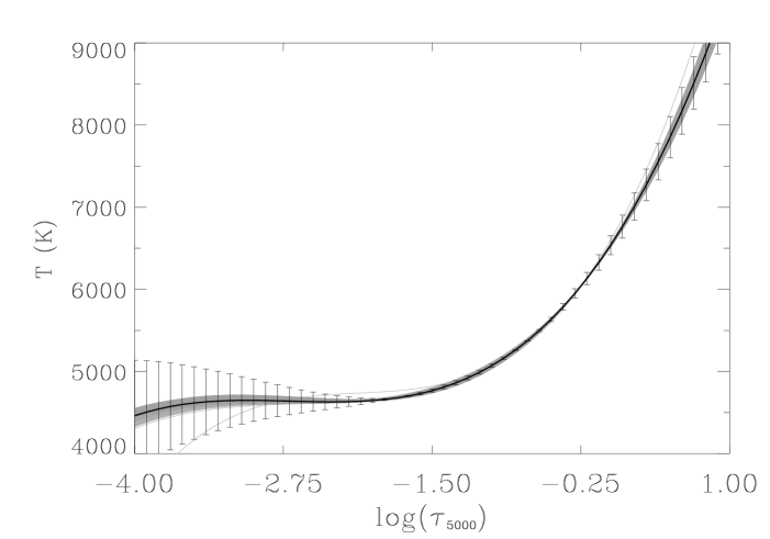
Figure 2: Temperature structures derived from the inversion of different datasets with different initial conditions (dotted gray lines). The discrepant case corresponds to one of the inversions with most extreme initial parameters ($\xi_{0}=0.5$ km s^-1 and $\Delta$ A = $-0.2$). The solid black curve with error bars corresponds to the inversion of all the available line profiles simultaneously.

As Figure 2 shows, the 120 atmospheric structures retrieved (dotted gray lines) are very similar to one another, and the scatter around the inversion of the whole database (solid black), is small. There is only a single renegade that corresponds to one of the eight data sets for $\xi_{0}=0.5$ km s^-1 and $\Delta$ A $=-0.2$. The error bars provided by the inversion code (see Appendix B in Sánchez Almeida 1997) seem to be slightly optimistic in the line forming region ($-2.0\leq\log\tau\leq-0.5$), whereas the scatter among the individual cases cannot be realistically associated to errors at depths where the inverted spectrum is not sensitive – at optical depths smaller than $\log\tau\sim-2.75$ and larger than $\log\tau\sim+0.5$ the thermal structure derived is just a extrapolation of neighbor depths that still affect the inverted spectrum, and in fact, some tests have shown that our formal error bars at extreme depths are unrealistically small. The main conclusion is that, as long as we provide an input spectrum able to constrain properly the thermal structure of the atmosphere, no matter which lines are used, we find a single solution.

Figure 3 answers the question of whether the recovered homogeneous atmosphere is some kind of average of the real three-dimensional structure. The recovered temperatures (solid line) show great resemblance to a temporal average of the simulation over layers of equal optical depth (dashed curve). This situation is totally different from the chromospheric case explored by Carlsson & Stein (1995), in which large fluctuations induced by waves on a cool-chromosphere solar model produced the same spectrum as a hydrostatic model with a hot-chromosphere. Even though at the temperatures of the solar photosphere the source function is typically on the non-linear (Wien) side of the Planck function, in this case there are no large fluctuations, and as a consequence, the thermal structure obtained from inversion of a time- and spatially-averaged spectrum is very close to the (linear) average of the 3D time-dependent atmosphere. The micro-turbulence retrieved by the inversions has a weak dependence on the initial value adopted ($\xi_{0}$), as can be seen in Figure 4. We recover a mean value $\xi=1.03\pm 0.02$ (1$\sigma$) km s^-1. The final macroturbulence is $1.58\pm 0.02$ km s^-1. This parameter was always initialized at 2.0 km s^-1, as it is much less relevant for the atmospheric structure.

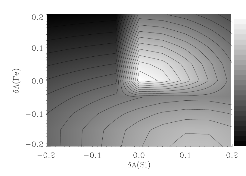
Figure 6: Response of the reduced $\chi^{2}$, normalized to its minimum value, to changes in the optimal abundances of iron and silicon. Both the gray scale and the contours use a logarithmic scale, and thus the units in the color-code bar are dex.

More interesting, although closely connected with the thermal structure, is the scatter among the retrieved abundances and its resemblance to the actual abundances used in the simulation. Figure 5 compares the histograms of the initial and final abundances for the 120 testing runs. The initial abundances correspond to the photospheric abundances of Anders & Grevesse (1989), with the abundances of Mg, Si, and Fe altered by $\Delta$ A $=0.0,\pm 0.1$ or $\pm 0.2$ dex, and their histogram corresponds to the spikes in each panel of the figure. The histogram of the final abundances is identified by the filled bars. The true abundances used in the simulation and three-dimensional radiative transfer are marked by asterisks in the figure. Table 3 gives the exact values used (GS98), as well as the weighted mean (and standard deviation) of the abundances recovered, labeled as ”A(Sim)”. The mean difference between true and recovered abundances is $-0.01\pm 0.02$ (SEM) dex, while the rms scatter is just 0.04 dex. Figure 6 displays the logarithm of the reduced $\chi^{2}$, normalized to its minimum, as a function of the variation in the abundances of iron and silicon from their optimal values [$\delta$A(Fe) and $\delta$A(Si)]. Changes of $\pm 0.2$ dex bring with them a degradation in the reduced $\chi^{2}$ by more than an order of magnitude.

The agreement is remarkable, given that the discrepancy between the true abundances and those used to initialize the inversion code reaches up to 0.4 dex, and that the inversion code tries to reproduce the input spectrum using a 1D representation, while the line formation is a highly non-linear process occurring in a 3D environment. The small differences of about 0.04 dex could well partly be attributed to the fact that continuum opacities, equation of state, partition functions, and other details are not exactly identical for the numerical simulations and the inversion code. This result gives confidence in the abundances derived from inversions working with homogeneous atmospheres. In the next section we attempt the inversion of the solar spectrum. Given this case of success, our prospects to derive reliable abundances are optimistic, although the practical application involves several error sources not present in the previous exercise, such as possible departures from LTE.

4 The solar spectrum

Inversions of the solar spectrum have already been presented by Allende Prieto et al. (1998) and Frutiger et al. (2000). Still, neither of them can be considered definitive. Both works were aimed at testing inversion techniques, rather than producing a serious analysis of the chemical abundances in the solar photosphere. Nonetheless, in view of the results from the previous section, this is indeed an interesting issue that deserves consideration.

We address the inversion of the solar flux spectrum armed with a carefully selected and comprehensive line list, which includes lines of the most important electron donors: Mg, Si, and Fe. Similarly to Allende Prieto et al. (1998), we extracted the observations from the solar atlas of Kurucz et al. (1984). Given that the inversion adopts a static model, the synthetic profiles are not able to reproduce the observed asymmetric line shapes, and thus it is unlikely that noise in the observed profiles is important, at least down to very low signal-to-noise ratios. But uncertainties in the atomic data could be an important source of error. We have selected radiative transition probabilities from the best sources in the literature, searching mainly for laboratory measurements, and we expect errors to be roughly symmetric. Redundancy, that is, including several lines that are formed over the same depth range, will then prevent organized errors. A symmetric error distribution might not be true for the adopted values for the natural damping, collected from VALD and likely coming from a single source (Kurucz’s theoretical calculations), but that parameter’s contribution is typically small, and definitely unimportant within a large sample.

As explained in §2, we have included wings of strong metal lines, which are expected to be weakly affected by departures from LTE and allow us to improve the depth coverage. An adequate treatment of collisional interactions with neutral hydrogen is crucial, because this is truly a potential source of systematic errors. The traditional Van der Waals approximation is by no means useful for this task, as it substantially underestimates the observed collisional damping to varying degrees. To the contrary, the studies in the literature that employed the Anstee, Barklem & O’Mara theories have proved this approach to be very promising (Asplund et al. 2000b; Barklem et al. 2000a). Fortunately, we do not need to take any risk. Our line database is sufficiently large and diverse that without the wings of strong metal lines we should have an adequate depth coverage. As a matter of fact, we can further test the collisional broadening theories by comparing inversions with, without, and only with, the wings of strong lines as input data.

We proceed with the inversion of the solar spectrum following the same scheme we applied for the 3D simulation. We carried out runs for each of the eight datasets with an initial micro-turbulence of $\xi_{0}=0.1,1.0,1.5$ and 2.0 km s^-1, always with $v_{\rm rot}\sin i=1.88$ km s^-1, and with the abundances of iron, magnesium and silicon simultaneously changed by $\Delta$ A $=-0.2,-0.1,0.0,+0.1$ and $+0.2$ dex, for a total of $8\times 4\times 5=160$ cases. All of them converged. Identically to the case of the simulation, we started out from an isothermal model with a macroturbulence of 2.0 km s^-1, progressively augmenting the complexity of the temperature structure. When attempting the inversion with seven nodes in temperature, wiggles started to appear, so the process was stopped after reaching six nodes. At the same time, the chemical abundances of the elements with lines in the input spectrum were allowed to change (taking into account their effect on the continuum opacities), and so was the depth-independent micro-turbulence. For a single run, the numbers of frequencies and lines were the same as in the inversion of the hydrodynamical simulation, because in §3 we used a mask to select the part of the profiles that would be useful in a real application. We also performed an inversion with all the lines simultaneously. Figure 7 shows some examples of the degree of agreement achieved between observed and synthetic profiles. It is interesting to mention that the global agreement between the input profiles and those produced by the atmosphere recovered by the inversion was slightly better for the simulation than for actual observations. Noticeably however, the wings of strong lines produced by the simulations could not be matched as well as those observed.

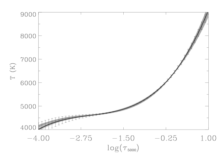
Figure 8: Temperature structures derived from the inversion of different datasets from the solar flux spectrum, with different initial conditions (dotted gray lines). The solid black with error bars corresponds to the inversion of all the available data simultaneously.

The temperature stratification of the 160 retrieved models is shown in Figure 8 (gray dotted lines). The black solid line with error bars corresponds to the run with all the lines simultaneously. Within the explored ranges, no matter the initial abundances or micro-turbulence, or which dataset of lines was involved, we arrive at a very narrow range of solutions. The model derived from the simultaneous inversion of all lines appears in Table 2.

The retrieved micro-turbulence is $1.1\pm 0.1$ km s^-1, quite independently from the value adopted as a starting guess ($\xi_{0})$, as shown in Figure 9. We find $1.54\pm 0.02$ km s^-1 for the macro-turbulence. We convolved the synthetic profiles with a Gaussian instrumental profile equivalent to the spectral resolution of the solar spectrum (R$\equiv\lambda/\delta\lambda\simeq 5\times 10^{5}$). We note that the value for the micro-turbulence we refer to corresponds to $\sqrt{2}\sigma$ of a Gaussian, (as traditionally used in the literature, e.g., Struve & Elvey 1934), the quoted value for the macro-turbulence corresponds to the $\sigma$ of a Gaussian, and the $\delta\lambda$ used to calculate the spectral resolution is the FWHM of the Gaussian instrumental profile ($\simeq 2.355\sigma$).

Figure 10 compares the histograms of the initial (spikes) and final (filled bars) abundances for the 160 testing runs. The initial abundances correspond to the photospheric abundances of Anders & Grevesse (1989), which for Mg, Si, and Fe are altered by $\Delta$ A $=0.0,\pm 0.1$ or $\pm 0.2$ dex, as indicated by the five spikes in the corresponding panels of the Figure. The asterisks show the revised photospheric values of GS98. The weighted mean (and standard deviation) of the abundances recovered for Mg, Si, Ca, Ti, Cr, and Fe are listed in Table 3, labeled with ”A(Obs)”. The agreement with GS98, what we can consider the commonly accepted values, is excellent, always within the uncertainties. Although having some overlap of the error bars, a slightly larger difference is found for Ti, whose meteoritic abundance (listed by Grevesse & Sauval: $4.94\pm 0.02$) is in better agreement with the value we find.

Apart from the quality with which the synthetic profiles fit the observations, which is limited by the line asymmetries, a rather interesting way to test the new model is to check for differences between the abundance of a given element as derived from lines with different atomic parameters. Rather than force all the lines of a given element to be fitted with a single abundance, we can find the abundance that best matches each observed profile and then check for trends against excitation potential (EP), equivalent width (EW), or wavelength ($\lambda$). We can fix the model structure and invert one line at a time, with the abundance of the corresponding element as the only parameter to be determined. Figure 11 shows that no trend is present when iron lines are considered. The filled and open symbols are used to distinguish neutral from ionized lines, and there is no difference between those two groups. The equivalent width in the second panel of the figure corresponds to the absorption produced by the part of the line profile used in the inversion, which is close to, or smaller than, the real equivalent width of the whole line profile. As the difference between the equivalent width used in the plot and the real equivalent width can be very large for the strong lines, we have limited the comparison in the middle panel to EW $<100$ mÅ. The solid lines are linear fits to the data, obtained by minimizing the $\chi^{2}$ error statistic, and the slopes of the abundance against EP, EW and wavelength are $(1\pm 12)\times 10^{-3}$, $(-8\pm 600)\times 10^{-6}$ and $(4\pm 11)\times 10^{-6}$, respectively, and therefore insignificant.

As a test of the continuum opacities, we removed all opacity sources except H^-, finding an atmospheric structure hardly distinguishable from the model in Table 2, and abundances that differed from those in Table 3 by less than 0.002 dex. Using our final solar model and abundances, we checked the influence of different approximations to estimate the lowering of the ionization potentials by Debye-Hückel shielding (see, e.g., Drawin & Felenbok 1965). Although different formulae predict very discrepant results, comparison of the most extreme estimates showed that this effect never alters the abundances of the considered species by more than 0.01 dex. The typical abundance shift for most of the lines of neutral species is about $-0.005$ dex, and it is much smaller and has the opposite sign for lines of singly-ionized species.

The profiles of the same lines we used from the solar atlas of Kurucz et al. (1984), were also extracted from the spectrum of the disk center included in the atlas of Neckel (Brault & Neckel 1987; Neckel 1999). The much smaller region of the disk that is averaged in the aperture, and the vertical view angle, produce sharper and much more asymmetric profiles, which are an even harder challenge for the symmetric profiles produced by the static model atmosphere. Figure 12 confirms that the recovered structure (dashed curve) is very similar to that derived from the flux spectrum (solid line with error bars), while the micro-turbulence is, understandably, smaller: 0.8 km s^-1. For reference, the empirical model published by Grevesse & Sauval (1999) is plotted with a dash-dotted line.

It is interesting to compare the model we found against theoretical models, which are widely used in astrophysical applications. Figure 13a compares the temperature structures derived by MISS with a MARCS model (Gustafsson et al. 1975; Asplund et al. 1997) with $T_{\rm eff}=5777$ K, $\log g=4.44$, and $\xi=1.00$ km s^-1, which uses the mixing length recipe to account for the convective flux and Grevesse & Sauval’s standard photospheric composition. The Grevesse & Sauval (1999) empirical model, based on a modification of the Holweger & Müller (1974) model, is also shown, and not surprisingly, is in much closer agreement with our model than the theoretical structure. The temperature of the theoretical model in the deepest layers is largely dependent on the particular choice for the parameters used in the mixing-length formulation. In particular, the differences between $-1<\log\tau<0.2$ are very important for astrophysical applications. The MARCS structure is up to 100 K cooler than MISS between $-1<\log\tau<0$, but hotter below $\log\tau\simeq 0$.

Figure 13b compares the models’ predictions against the flux measured in the optical and near-IR, as critically compiled by Colina, Bohlin & Castelli (1996). At wavelengths shorter than $\sim$ 600 nm the abundance of absorption lines depresses the observed flux, and makes this comparison meaningless. Colina et al. concluded that the observations available for wavelengths longer than 960 nm are affected by large systematic errors and, therefore, we discarded that region from the comparison. The large high frequency scatter is produced by line absorption in the solar atmosphere, whereas the low frequency variations are mostly associated with broad absorptions in the Earth’s atmosphere. Surprisingly, the fluxes predicted by the two models are closer than expected from the differences in their thermal structures. Discrepancies in the continuum opacities and/or the equation of state used by MISS and MARCS solve the potential problem. Such discrepancies should be responsible at least for a share of the differences in temperature between the two models, and deserve further investigation, although they are certainly outside of the scope of this paper.

5 Completeness and redundancy in the input data

From the convergence to very similar structures of inversions with eight different datasets, all of them including weak-neutral, weak-ionized, and strong lines, it is apparent that each dataset provides very similar information about the solar photosphere. A practical question immediately arises. Are all the lines necessary? We are interested in knowing what features contain most of the information and whether it is possible to use only a few, carefully selected, lines to recover the photospheric structure.

Using an inversion procedure like MISS, we can only determine the atmospheric parameters that directly or indirectly affect the formation of the input spectral lines. Basically, the thermal structure, the chemical abundances, and the micro-turbulence are the most important parameters controlling the overall strength of the metal lines. Temperature, gas pressure, and (micro/macro) turbulence affect the line width. Any of the aforementioned parameters has a different impact on a given spectral line profile, but some parameters’ influence on that particular line may be very similar. If our description of the atmosphere and the line formation were perfect, ideal observations of a single profile would suffice to disentangle every parameter at play. However, the use of a simplified model atmosphere, the presence of noise in observations and atomic data, plus the inclusion of a long list of approximations, make up a much more complicated situation. In practice, for any given line, there is a degeneracy between some parameters, but it can avoided by including other lines with different sensitivity:

• Weak lines cover a limited range of depths, so a set of different lines is required to constrain tightly the thermal structure. Strong lines span a larger range of opacity, even just along their wings, and consequently, they provide more information. Figure 14a compares the temperature structures recovered from all the lines (solid curve with error bars), only weak lines (dashed) and only strong lines (dashed-dotted). We also found that reducing the number of weak lines by a factor of two already compromises the depth coverage. Basically, the information provided by the 55 weak lines is also contained in the set of 7 strong lines.

  When the number of lines used becomes small, there is little place for errors in the atomic data. More importantly, the fact that the atmosphere retrieved from only strong lines is virtually identical to that from a large number of weak lines highlights that the pressure-broadening by collisions with hydrogen atoms is properly described by the theories of Anstee, Barklem & O’Mara, at least for the lines used here. The difference between the abundances derived from only-weak and only-strong lines are 0.03 and 0.00 dex, for calcium and iron respectively.

• It is possible to compensate a change in the chemical abundance that produces a given line through a change in temperature. Several lines of the same species are unlikely to be sufficient to solve this issue, as their different responses to a fractional change of the abundance could be compensated by a particular thermal structure. A combination of lines of different species will break down the temperature-abundance degeneracy. Lines produced by different ionization stages of the same element will have similar sensitivity to changes in the abundance, but if one of the species is the dominant, they will typically show opposite responses to an increase or decrease of the temperature. Logically, lines of different elements may have similar responses to the temperature, but not to any of their abundances. The temperature-abundance degeneracy can be exemplified by an inversion restricted to only neutral or ionized lines. The dashed line in Fig. 14b corresponds to the thermal structure derived from only neutral lines, the dashed-dotted line was obtained from only ionized lines, and the solid curve with error bars was derived with all, neutral and ionized lines. The different thermal structures bring with them changes in the chemical abundances of up to 0.1 dex, not always in the same sense for all the elements. Additionally, the micro-turbulence changes slightly (0.8 and 1.1 km s^-1 for the only-neutral and only-ionized cases, compared to 1.1 km s^-1) and so does the macroturbulence ($+0.1$ and $+0.2$ km s^-1).

• By definition, the micro-turbulence represents small-scale velocity fields. If, as in our case, those are assumed isotropic and Gaussian, it is very difficult to distinguish between thermal and small-scale turbulent velocities. This gives place to a second degeneracy, which involves temperature and micro-turbulence. Micro-turbulence cannot, however, mimic the effect that temperature has on the lines, but if the abundance can change freely to accommodate any variation of temperature, we are set for confusion. Including lines of the same element with opposite sensitivity to variations in temperature will automatically constrain that variable. Several lines of a given single species could in principle be useful, as moderately weak and moderately strong lines are sensitive to micro-turbulence, but the wings of very strong lines (such as the Ca II lines in Table 1) are not affected by this parameter. In practice, different ionization stages of the same element are still necessary, as otherwise it is not possible to break down the abundance-temperature degeneracy. This is well illustrated by an inversion of all the strong lines, only strong lines of neutral species, and only strong lines of ionized species. In Fig. 14c, the solid line was obtained from the inversion of all the strong lines – as we have seen, virtually indistinguishable from the inversion of all, weak and strong lines. The dashed curve was derived from only strong lines of neutral species, whereas the dashed-dotted curve from only strong lines of ionized species. The disparity between the thermal structures corresponds to differences in the derived abundances that can reach up to 0.3 dex. The key to the success of the inversion with only a few strong lines resides in the presence of two lines of different species of calcium in our list of strong lines.

  It is interesting to explore whether the group of strong lines suffices to constrain the micro-turbulence and, therefore, to confirm that they are able to retrieve the temperature structure without any previous knowledge about the micro-turbulence. A set of 20 experiments corresponding to $\xi_{0}=0.5,1.0,1.5$, and 2.0 km s^-1 and $\Delta$A $=-0.2,-0.1,0.0,+0.1$, and $+0.2$ dex for Mg, Si, and Fe, was set, finding that the structures were very similar, and the final micro- and macro-turbulence velocities had a mean value of $1.18\pm 0.02$ km s^-1 and $1.86\pm 0.02$ km s^-1, respectively. As an example of the impact of the scatter on the abundances, we found a mean value for the iron abundance of $7.500\pm 0.004$ (SEM) dex, with a standard deviation of 0.02 dex. Although the strongest lines in the group, Ca II at 8542 and 8662 Å, are unreactive to the micro-turbulence, the other strong, but weaker, lines are quite sensitive to this parameter.

With only lines of neutral species, Allende Prieto et al. (1998, 2000) used the goodness-of-fit between synthetic and observed line profiles as a criterion to determine the micro-turbulence. It has, however, become apparent from our experiments that lines of different ionization stages are needed to solve properly the inversion problem.

Hydrogen lines would be a particularly interesting tool to analyze the spectra of solar-like stars. With H^- as the dominant source of continuum opacity, the strength of hydrogen lines is a fine sensor for the atmospheric thermal structure. Spanning a dramatic range in opacity, a single hydrogen line might be useful to obtain information from the whole photosphere, even extending the depth coverage provided by our present database. Nonetheless, at this point we have not considered the use of hydrogen lines in inversions because their broadening is extremely complex. This complexity is apparent in that it is not possible to reconcile the effective temperatures obtained from the Balmer lines with other indicators, such as the Infrared Flux Method (Fuhrmann et al. 1993; Alonso et al. 1996). We note that new theoretical developments might change this situation in the near future (Barklem et al. 2000b, c).

6 Practicalities of the application of inversion methods to other stars

From the inversion of the hydrodynamical solar simulation, we have found that systematic errors in the abundances from single-component homogeneous inversions of solar-like spectra are likely about 10 % (0.04 dex). From our inversions of the solar spectrum, we have seen that random errors can be a factor of two smaller, provided we carry out a careful selection of the input data. This kind of accuracy is sufficient for many applications.

Stellar spectra are typically acquired with lower resolution and signal-to-noise ratio than solar spectra, and it is necessary to assess the resistance of the inversion procedure to these factors. In most cases the stellar gravity is not known with much precision, but we need this parameter to derive the pressure gradient from the thermal structure. Finally, unlike the solar case, the projected rotational velocity of the star is unknown a priori. Unless one of them is significantly larger than the other, it is likely that there will be some confusion between rotation and macro-turbulence. All these issues are explored below.

6.1 Lower resolution and signal-to-noise ratio

A spectral line produced in a one-dimensional static atmosphere cannot reproduce the line asymmetries observed in real spectra. The synthetic profiles obtained by our inversion procedure will not match the detailed shape of the observed lines, which gives us a hint that we might not need to resolve such details in the observed input spectra. It is also true that if we try to minimize the difference between observed and synthetic spectra, introducing some noise with a symmetric distribution will not affect the $\chi^{2}$. In practice, degrading signal-to-noise and resolution comes with a series of additional problems. First, it becomes harder to identify spectral features associated to a single transition. Second, it gets more difficult to normalize the spectrum, and to determine where the center of a line is. Third, the number of spectral points with independent information diminishes, and so does the available information.

To check the resistance of the inversion method against a degradation in the signal-to-noise ratio and resolution, we have made use of the dataset from the solar spectrum used in previous sections. We first resampled the spectrum to have two wavelengths per resolution element, then we degraded the spectrum by convolving it with a Gaussian profile, and resampled it to have two wavelengths per resolution element again. We generated random numbers following a Poisson distribution (centered at 1 and scaled to the appropriate width) which were multiplied by the spectrum. Finally, every single line was recentered before entering into the inversion code. For practical reasons, all the processing was done with the full observed profiles, so at the end we applied the same mask used in the solar inversions to exclude wavelengths apparently affected by blends. We tried two different values for the final resolving power (R$=1\times 10^{5}$ and $5\times 10^{4}$) and two for the signal-to-noise ratio (SNR $=100$ and 33).

Figure 15 shows the structure derived in §4 from the original solar spectrum (solid line) and the new four inversions of the degraded spectra. In accordance with the small effect on the thermal structure, the abundances are affected very little; the iron abundances obtained for (SNR = 100, R = $10^{5}$), (SNR = 100, R = $5\times 10^{4}$), (SNR = 33, R = $10^{5}$), and (SNR = 33, R = $5\times 10^{4}$) are 7.50, 7.51, 7.50, and 7.52, respectively. The tests suggests that a correct inversion is still possible with a resolution and a signal-to-noise ratio as low as $5\times 10^{4}$ and $33$, respectively. At these levels, the weakest lines are simply dissolved in the noise and mapped with a few points. However, as we have seen, the strongest lines of the spectrum already contain all the information, and those features are very resistant to the decline in resolution and signal-to-noise ratio.

6.2 Uncertainties in gravity

The surface gravity of the Sun is a well-known parameter, $\log g=4.437368\pm 0.000087$ (Stix 1991), even if it might suffer larger variations than its formal error bar indicates depending on which definition of radius is used. The overall sensitivity of the spectrum to changes in gravity is relatively small, compared to temperature, so in this regard an uncertainty in $\log g$ smaller than 0.05 dex is normally sufficient. For stars closer than about 100 pc, it is possible to combine accurate trigonometric parallaxes with calculations of stellar evolution, constraining $\log g$ within roughly 0.06 dex (Allende Prieto & Lambert 1999). For other stars, gravities are usually determined from spectroscopic analysis or spectroscopic classification, rarely achieving a precision better than about 0.2 dex, in some cases with much larger systematic errors (Allende Prieto et al. 1999). Definitely, it is important to check how sensitive the results of an inversion are to uncertainties in gravity.

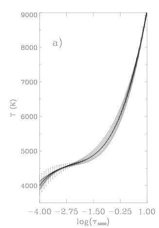
Figure 16: a): Thermal structures derived adopting the real solar gravity ($\log g=4.44$; thick line) and lower and higher values by $\Delta\log g=-0.3,-0.2,-0.1,+0.1,+0.2,+0.3$ dex. A cooler temperature stratification tries to compensate for a wrongly set lower gravity. b): The micro- ($\xi$) and macro-turbulence ($v_{\rm mac}$) as a function of the assumed gravity for the solar inversion. These two parameters, together with the temperature structure and the abundances, are affected by setting the gravity wrongly. c): Quality of the fit to the input line profiles, quantified by the sum of the square differences between observed and synthetic normalized fluxes, as a function of the fixed surface gravity. The solid line represents a least-square fit to a second-order polynomial.

We have repeated the inversion of the solar data used in §4 but adopting a value for the gravity which is different from solar by $-0.3,-0.2,-0.1,+0.1,+0.2$, and $+0.3$ dex. The effect on the recovered thermal structure is shown in Figure 16a. The thick curve corresponds to the solution for the right gravity and the thinner lines were derived for the other values. Dropping the gravity is compensated by decreasing the temperature and likewise higher gravities lead to hotter models. Figure 16b shows that the turbulent velocities derived from the inversion are also shifted with the gravity (note that $v_{\rm rot}\sin i$ is always held as a known parameter).

In Figure 16c we take a close look at the relative quality of the fits for the different $\log g$ values, quantified by the sum of the square differences between the observed and synthetic normalized fluxes. The best fit is found for gravities close to the real value, revealing that it is possible to extract the gravity from the inversion. This suggests adding the gravity to the pool of free parameters to determine in the inversion. Frutiger et al. (2000) did so, but they recovered $\log g$ values for $\alpha$ Cen B systematically $0.2-0.4$ dex higher than the value derived by Allende Prieto & Lambert (1999) based on the trigonometric parallax. The most recent version of MISS does not incorporate gravity as a free parameter, but we will explore this promising possibility in the future.

As shown in Figure 17, the changes in the atmospheric structures derived for different gravities are accompanied with variations in the abundances. The abundances have sensitivities that reach up to about 0.2 dex per dex (for an uncertainty in the $\log g$ of $\sim 0.2$ dex, some abundances may be wrong by 0.04 dex). Though these are not very large errors, they would double the systematic errors associated with the assumption of a plane-parallel hydrostatic atmosphere studied in §3.

6.3 Rotation and macroturbulence

If the gravity is usually uncertain, the rotational velocity is completely unknown. For a spherically symmetric star without surface features, all we can aspire to deduce from the spectral lines is the product $v_{\rm rot}\sin i$. In many cases, not even that, as disentangling rotation from other competing broadening mechanisms is not trivial. The projected rotational velocity can be combined with other sources of information to extract the angular velocity, which is by itself an important parameter as it affects the star’s structure and evolution.

To learn what the prospects are for the inversion to obtain accurate projected rotational velocities, whether rotation can be confused with other velocity fields with smaller characteristic length-scales (macro-turbulence), and the possible influence that such confusion would have on the retrieved abundances, we have introduced rotation as a free parameter in dealing with the solar spectrum. We have carried out inversions with an initial guess $(v_{\rm rot}\sin i)_{0}$ of 1, 2, 3, and 4 km s^-1. The solid lines in Figure 18a show the recovered $v_{\rm rot}\sin i$, $v_{\rm mac}$, $\xi$, and the sum of $v_{\rm rot}\sin i+v_{\rm mac}$, whereas the dashed line shows the reduced $\chi^{2}$, adopting $\sigma_{i}=1$, for each final solution (the particular value of $\sigma_{i}$ does not matter, as we are interested in relative values). The sum of the macro-turbulence and the projected rotational velocity is roughly conserved, but that does not apply for each of the two line broadening components.

We are not very surprised by this result. A Gaussian isotropic macro-turbulence is not a very good description of the atmospheric large-scale convective motions (Asplund et al. 2000a), and in the solar case macro-turbulence and projected rotational velocity happen to be of similar size, further complicating their separation. A homogeneous model atmosphere cannot reproduce the asymmetric spectral lines produced by convective turbulence, limiting the information we are able to extract from the detailed shapes of the line profiles. It is possible that a different description of turbulence, such as the radial-tangential recipe (Gray 1975) could be useful to improve these results. It might be possible as well that homogeneous models with two or more components and depth-dependent velocities could be useful to this end. At this time we do not have an answer, but it is worthwhile to explore this issue more deeply.

Figure 18b shows that the shape of the atmospheric structures has almost no dependence on the final rotational velocity. Consequently, the retrieved abundances are also very weakly affected. The standard deviations of the abundances of Si, Ca, Ti, Cr and Fe found for the four different values of $(v_{\rm rot}\sin i)_{0}$ are less than or about 0.01 dex. As our data includes a single Mg line, the abundance of this element is much more sensitive, showing a standard deviation of 0.04 dex.

7 Conclusions and prospects

There are two major difficulties to describe accurately the energy balance in the atmospheres of late-type stars: line blanketing and convection. Line blanketing is a problem because it requires including a very large number of frequencies, and the atomic data for many lines is uncertain or unavailable. Convection accounts for a significant part of the energy transferred outwards in the deepest photospheric layers, and the simplistic approaches to take it into account within the framework of static and homogeneous models have many free parameters. A proper description of convection has been achieved through numerical hydrodynamical modeling (Stein & Nordlund 1998, Asplund et al. 2000a), but this is computationally very involved, and currently impractical for carrying out chemical analyses of large samples of stars.

A possible way to bypass the theoretical annoyance is to use observations to constrain as many parameters as possible, rather than just a few. Inversion methods can be applied to stellar spectra and so relax some theoretical assumptions. In the interleaved measuring-modeling process that is used to determine chemical abundances from stellar spectra, these methods try to effectively shift the balance towards a pure measurement. Among these codes, MISS (Allende Prieto et al. 1998) adopts a one-dimensional single-component model atmosphere in LTE and hydrostatic equilibrium.

Recent calculations show that departures from LTE in the photospheres of solar-like stars are, on average, relatively small both in the line formation (Shchukina & Trujillo Bueno 2001, Gehren et al. 2001) and in the photospheric structure (Hauschildt, Allard, & Baron 1999). Shchukina & Trujillo Bueno (2001) find that assuming LTE can artificially decrease the mean iron abundance obtained from the analysis of Fe I intensity profiles with a three-dimensional model atmosphere by $\sim 0.07$ dex, and with the Holweger & Müller solar model by $\sim$ 0.06 dex. If this is right, a non-LTE line-formation analysis of iron in 1D would provide accurate corrections to $\sim 0.01$ dex. However, a previous calculation by Thévenin & Idiart (1999) found that typical errors in the LTE abundances from disk-integrated observations analyzed with homogeneous solar model atmospheres were essentially zero. The differences between these two works might reside in the fact that Shchukina & Trujillo Bueno used intensity, whereas Thévenin & Idiart employed flux, the particular lines employed, or the atomic data adopted. We should emphasize that depending on which element is studied, the specifics of the atmosphere, and the particular set of spectral lines employed, non-LTE corrections may be large, and also may differ significantly for 3D and 1D calculations (see, e.g., lithium in metal-poor dwarfs; Asplund et al. 1999).

We have tried to fill an important gap, as there was no quantitative assessment of the systematic errors incurred by the use of a static and homogeneous model atmosphere as part of an inversion method. In our experiment, we removed non-LTE effects by adopting LTE in both the synthesis of the profiles emerging from the simulation and in the inversion. We have employed a detailed three-dimensional time-dependent hydrodynamical simulation of the solar surface to calculate a spatial-, angular- and time-averaged spectrum, which has been fed to MISS. The rms difference between the abundances recovered by the inversion code and those used in the three-dimensional simulation was only 10 % (0.04 dex), and the mean difference was $-0.01\pm 0.02$ (SEM) dex. Speaking generally, it is apparent that even with the worst expectations, departures from LTE will not make this error much larger than 0.07 dex. This kind of accuracy is sufficient for many applications. From our inversions of the solar spectrum, we have seen than internal random errors can be reduced to about 0.02 dex, provided we carry out a careful selection of the input data.

We have compiled a careful selection of spectral features of Mg, Si, Ca, Ti, Cr, and Fe, including strong lines for which calculations of the collisional damping due to neutral hydrogen are available. Normalized line profiles are used to carry out an inversion of the solar spectrum, searching for the chemical abundances of the involved elements, a depth-independent micro-turbulence, a Gaussian macro-turbulence, and the atmospheric thermal structure, that reproduce the observations best. There are no surprises, the abundances recovered are similar to the commonly accepted values listed by Grevesse & Sauval (1998).

We realize that a very limited number of strong lines from different ionization stages suffices to constrain the atmospheric structure and the abundances. In fact, we tested our inversion procedure against a degradation of the spectral resolution and signal-to-noise ratio in the data, finding that reliable inversions are possible at R $\equiv\lambda/\delta\lambda\sim 5\times 10^{4}$ and SNR $\sim 30$. The stellar gravity, usually poorly determined, can also be recovered by the inversion. However, the projected rotational velocity and the Gaussian macro-turbulence are easily confused when their size is similar, but this has a very small effect on the abundances, at least for the solar case.

With these new results, we foresee no major difficulty to make use of inversions of stellar spectra to perform extensive analysis of chemical abundances in stars with solar or similar temperatures and metallicities. Further and in progress development of our code for this task includes a more detailed treatment of the macro-turbulence (expected to be useful in separating macro-turbulence and rotation), the addition of a second one-dimensional component, and vertical velocities, to the model atmosphere (aimed at extracting information on the granulation and achieving a closer match of the observations), and the addition of gravity to the pool of parameters to be determined automatically.

Further extension of tests like the one described in this paper, and on departures from LTE, to other domains in the HR diagram are also in progress and will be the subject of forthcoming papers. So far, we should mention that there is evidence of much larger systematic effects for stars slightly warmer than the Sun. For example, in a three-dimensional simulation for Procyon ($T_{\rm eff}\simeq 6500$ K) the layers with the largest temperature inhomogeneities overlapped with the continuum-forming region, whereas in the solar simulation such layers are below the continuum-forming region (Nordlund & Dravins 1990, Allende Prieto et al. 2001). Hauschildt et al. (1999) detected large departures from LTE, even affecting the calculation of the (horizontally-homogeneous) atmospheric structure, for a star like Vega ($T_{\rm eff}\simeq 10,000$ K). Evidence is also present for larger-than-solar inhomogeneities in metal-deficient stars (Allende Prieto et al. 1999, Asplund et al. 1999), as it is for larger-than-solar departures from LTE (Thévenin & Idiart 1999).

Table 1: Spectral lines and atomic data used in the inversion. Cross-sections $\sigma$ for the collisional broadening by hydrogen are given for $v=10^{4}$ m s^-1, and $\alpha$ describes the velocity dependence assuming $\sigma(v)\propto v^{-\alpha}$

Species	Wavelength	$E_{\mathrm{low}}$	$\log(gf)$	$\sigma$	$\alpha$	$\log\Gamma_{\mathrm{rad}}$	$\log(gf)$ source
	(Å)	(eV)		($a_{0}^{2}$)		(rad s-1)
Weak–Neutral
Si I	5665.557	4.92	$-$1.940	1772	0.222	8.290	BZH
Si I	5684.490	4.95	$-$1.550	1798	0.221	8.250	BZH
Si I	5690.425	4.93	$-$1.770	1772	0.222	8.300	BZH
Si I	5701.106	4.93	$-$1.950	1768	0.222	8.310	BZH
Si I	5708.402	4.95	$-$1.370	1787	0.222	8.270	BZH
Si I	5948.545	5.08	$-$1.130	1845	0.222	8.330	BZH
Si I	7680.271	5.86	$-$0.590	2107	0.495	7.660	BZH
Si I	7918.387	5.95	$-$0.510	2934	0.232	7.530	BZH
Si I	7932.356	5.96	$-$0.370	2985	0.235	7.570	BZH
Ca I	6161.297	2.52	$-$1.266	978	0.257	7.274	Oxford
Ca I	6166.441	2.52	$-$1.142	976	0.257	7.269	Oxford
Ca I	6455.604	2.52	$-$1.290	365	0.241	7.667	Oxford
Ca I	6499.656	2.52	$-$0.818	364	0.239	7.640	Oxford
Ti I	4758.122	2.25	0.481	326	0.246	8.029	GBP
Ti I	4759.274	2.25	0.570	327	0.246	8.029	GBP
Ti I	5113.445	1.44	$-$0.727	298	0.243	7.332	GBP
Ti I	5295.781	1.05	$-$1.577	278	0.253	6.687	GBP
Ti I	5490.154	1.46	$-$0.877	374	0.262	8.155	GBP
Ti I	5866.457	1.07	$-$0.784	259	0.262	7.643	GBP
Ti I	5922.115	1.05	$-$1.410	313	0.242	7.853	GBP
Ti I	6092.799	1.89	$-$1.323	398	0.239	8.104	GBP
Ti I	6258.109	1.44	$-$0.299	355	0.237	8.230	GBP
Ti I	7357.735	1.44	$-$1.066	329	0.244	7.846	GBP
Cr I	4801.028	3.12	$-$0.131	348	0.240	7.857	Oxford
Cr I	4964.931	0.94	$-$2.527	262	0.261	8.236	Oxford
Cr I	5272.002	3.45	$-$0.422	757	0.238	8.401	Oxford
Cr I	5300.751	0.98	$-$2.129	329	0.263	7.716	Oxford
Cr I	5312.859	3.45	$-$0.562	751	0.238	8.402	Oxford
Cr I	5787.922	3.32	$-$0.083	1097	0.291	8.002	Oxford
Cr I	7355.899	2.89	$-$0.285	902	0.246	7.822	Oxford
Fe I	4602.006	1.61	$-$3.150	296	0.260	8.083	Oxford
Fe I	5225.533	0.11	$-$4.790	207	0.253	3.643	Oxford
Fe I	5247.057	0.09	$-$4.950	206	0.253	3.894	Oxford
Fe I	5916.254	2.45	$-$2.990	341	0.238	8.009	Oxford
Fe I	5956.700	0.86	$-$4.610	227	0.252	4.433	Oxford
Fe I	6082.715	2.22	$-$3.570	306	0.271	6.886	Oxford
Fe I	6151.623	2.18	$-$3.300	277	0.263	8.190	Oxford
Fe I	6173.342	2.22	$-$2.880	281	0.266	8.223	Oxford
Fe I	6200.321	2.61	$-$2.440	350	0.235	8.013	Oxford
Fe I	6297.801	2.22	$-$2.740	278	0.264	8.190	Oxford
Fe I	6481.878	2.28	$-$2.980	308	0.243	8.190	Oxford
Fe I	6498.945	0.96	$-$4.700	226	0.253	4.638	Oxford
Fe I	6750.161	2.42	$-$2.620	335	0.241	6.886	Oxford
Fe I	6978.861	2.48	$-$2.500	337	0.241	6.886	Oxford
Weak–Ionized
Si II	6371.361	8.12	$-$0.000	389	0.189	9.080	BZH
Ti II	4798.535	1.08	$-$2.670	211	0.209	8.283	BHN
Ti II	5336.793	1.58	$-$1.630	272	0.314	8.207	BHN
Ti II	5418.773	1.58	$-$2.110	270	0.315	8.199	BHN
Fe II	4508.287	2.84	$-$2.520	188	0.267	8.617	PGH Resc.
Fe II	4656.979	2.88	$-$3.580	190	0.330	8.612	HK Resc.
Fe II	5234.632	3.21	$-$2.230	188	0.268	8.487	HK Resc.
Fe II	6432.684	2.89	$-$3.510	174	0.270	8.462	SKH
Fe II	6516.086	2.89	$-$3.380	174	0.270	8.464	SKH
Fe II	7515.836	3.90	$-$3.450	187	0.271	8.612	PGH, HK Aver. Resc.
Fe II	7711.730	3.90	$-$2.450	186	0.264	8.615	PGH, HK Aver. Resc.
Strong
Mg I	8806.778	4.33	$-$0.120	531	0.292	8.690	RS
Ca I	6162.183	1.89	$-$0.097	878	0.236	7.860	Oxford
Ca II	8542.120	1.70	$-$0.463	291	0.275	8.164	THE
Ca II	8662.169	1.69	$-$0.723	291	0.275	8.152	THE
Fe I	5232.952	2.94	$-$0.058	713	0.238	8.009	OWL
Fe I	8327.067	2.20	$-$1.525	258	0.247	7.303	Oxford
Fe I	8688.643	2.17	$-$1.212	253	0.245	7.276	Oxford

References. — Sources of $f$-values: BZH = Becker, Zimmermann, & Holweger (1980); BHN = Bizzarri et al. (1993); GARZ = Garz (1973); GBP = Grevesse, Blackwell & Petford 1989; HLG = Hannaford et al. (1992); HK = Heise & Kock (1990); OWL = O’Brian et al. (1991); Oxford = Blackwell & Shallis (1979) and following papers; Pauls, Grevesse, & Huber (1990); RS = Ruck & Smith (1993); SKH = Schnabel, Kock, & Holweger (1999); THE = Theodosiou (1989)

Note. — Aver. = averaged ; Resc. = Rescaled to averaged lifetime of Schnabel et al. (1999) and Guo et al. (1992)

Table 2: Solar model atmosphere derived from the inversion

$\log\tau_{5000}$	T	Pe	Pg	$\rho$	column mass
	(K)	(dyn cm-2)	(dyn cm-2)	(g cm-3)	(g cm-2)
$-$4.0	4003.8	0.2636$\times 10^{-01}$	0.2903$\times 10^{+03}$	0.1132$\times 10^{-08}$	0.0000$\times 10^{+00}$
$-$3.9	4081.5	0.4348$\times 10^{-01}$	0.4798$\times 10^{+03}$	0.1835$\times 10^{-08}$	0.9047$\times 10^{-02}$
$-$3.8	4151.3	0.6163$\times 10^{-01}$	0.6705$\times 10^{+03}$	0.2521$\times 10^{-08}$	0.1714$\times 10^{-01}$
$-$3.7	4214.0	0.8146$\times 10^{-01}$	0.8715$\times 10^{+03}$	0.3228$\times 10^{-08}$	0.2524$\times 10^{-01}$
$-$3.6	4270.1	0.1033$\times 10^{+00}$	0.1089$\times 10^{+04}$	0.3979$\times 10^{-08}$	0.3374$\times 10^{-01}$
$-$3.5	4320.0	0.1274$\times 10^{+00}$	0.1326$\times 10^{+04}$	0.4791$\times 10^{-08}$	0.4288$\times 10^{-01}$
$-$3.4	4364.3	0.1540$\times 10^{+00}$	0.1588$\times 10^{+04}$	0.5678$\times 10^{-08}$	0.5285$\times 10^{-01}$
$-$3.3	4403.5	0.1834$\times 10^{+00}$	0.1878$\times 10^{+04}$	0.6658$\times 10^{-08}$	0.6385$\times 10^{-01}$
$-$3.2	4438.2	0.2159$\times 10^{+00}$	0.2202$\times 10^{+04}$	0.7745$\times 10^{-08}$	0.7605$\times 10^{-01}$
$-$3.1	4469.2	0.2520$\times 10^{+00}$	0.2565$\times 10^{+04}$	0.8959$\times 10^{-08}$	0.8966$\times 10^{-01}$
$-$3.0	4496.9	0.2919$\times 10^{+00}$	0.2971$\times 10^{+04}$	0.1031$\times 10^{-07}$	0.1049$\times 10^{+00}$
$-$2.9	4521.2	0.3362$\times 10^{+00}$	0.3429$\times 10^{+04}$	0.1184$\times 10^{-07}$	0.1220$\times 10^{+00}$
$-$2.8	4543.6	0.3853$\times 10^{+00}$	0.3942$\times 10^{+04}$	0.1354$\times 10^{-07}$	0.1412$\times 10^{+00}$
$-$2.7	4564.2	0.4400$\times 10^{+00}$	0.4521$\times 10^{+04}$	0.1546$\times 10^{-07}$	0.1629$\times 10^{+00}$
$-$2.6	4583.6	0.5008$\times 10^{+00}$	0.5172$\times 10^{+04}$	0.1761$\times 10^{-07}$	0.1874$\times 10^{+00}$
$-$2.5	4602.3	0.5688$\times 10^{+00}$	0.5906$\times 10^{+04}$	0.2003$\times 10^{-07}$	0.2150$\times 10^{+00}$
$-$2.4	4620.8	0.6451$\times 10^{+00}$	0.6737$\times 10^{+04}$	0.2275$\times 10^{-07}$	0.2463$\times 10^{+00}$
$-$2.3	4639.9	0.7309$\times 10^{+00}$	0.7672$\times 10^{+04}$	0.2581$\times 10^{-07}$	0.2817$\times 10^{+00}$
$-$2.2	4659.7	0.8277$\times 10^{+00}$	0.8729$\times 10^{+04}$	0.2924$\times 10^{-07}$	0.3219$\times 10^{+00}$
$-$2.1	4681.6	0.9380$\times 10^{+00}$	0.9923$\times 10^{+04}$	0.3308$\times 10^{-07}$	0.3675$\times 10^{+00}$
$-$2.0	4705.1	0.1064$\times 10^{+01}$	0.1128$\times 10^{+05}$	0.3741$\times 10^{-07}$	0.4193$\times 10^{+00}$
$-$1.9	4731.3	0.1209$\times 10^{+01}$	0.1281$\times 10^{+05}$	0.4227$\times 10^{-07}$	0.4781$\times 10^{+00}$
$-$1.8	4760.9	0.1376$\times 10^{+01}$	0.1455$\times 10^{+05}$	0.4768$\times 10^{-07}$	0.5449$\times 10^{+00}$
$-$1.7	4793.8	0.1571$\times 10^{+01}$	0.1652$\times 10^{+05}$	0.5380$\times 10^{-07}$	0.6209$\times 10^{+00}$
$-$1.6	4831.2	0.1800$\times 10^{+01}$	0.1878$\times 10^{+05}$	0.6067$\times 10^{-07}$	0.7072$\times 10^{+00}$
$-$1.5	4873.4	0.2069$\times 10^{+01}$	0.2134$\times 10^{+05}$	0.6833$\times 10^{-07}$	0.8055$\times 10^{+00}$
$-$1.4	4920.8	0.2388$\times 10^{+01}$	0.2425$\times 10^{+05}$	0.7693$\times 10^{-07}$	0.9171$\times 10^{+00}$
$-$1.3	4974.3	0.2769$\times 10^{+01}$	0.2758$\times 10^{+05}$	0.8654$\times 10^{-07}$	0.1044$\times 10^{+01}$
$-$1.2	5034.2	0.3227$\times 10^{+01}$	0.3138$\times 10^{+05}$	0.9727$\times 10^{-07}$	0.1188$\times 10^{+01}$
$-$1.1	5101.0	0.3784$\times 10^{+01}$	0.3572$\times 10^{+05}$	0.1093$\times 10^{-06}$	0.1352$\times 10^{+01}$
$-$1.0	5174.9	0.4469$\times 10^{+01}$	0.4071$\times 10^{+05}$	0.1228$\times 10^{-06}$	0.1538$\times 10^{+01}$
$-$0.9	5257.8	0.5328$\times 10^{+01}$	0.4637$\times 10^{+05}$	0.1377$\times 10^{-06}$	0.1747$\times 10^{+01}$
$-$0.8	5348.7	0.6427$\times 10^{+01}$	0.5284$\times 10^{+05}$	0.1542$\times 10^{-06}$	0.1982$\times 10^{+01}$
$-$0.7	5449.1	0.7879$\times 10^{+01}$	0.6018$\times 10^{+05}$	0.1724$\times 10^{-06}$	0.2243$\times 10^{+01}$
$-$0.6	5559.0	0.9866$\times 10^{+01}$	0.6852$\times 10^{+05}$	0.1924$\times 10^{-06}$	0.2528$\times 10^{+01}$
$-$0.5	5679.5	0.1268$\times 10^{+02}$	0.7790$\times 10^{+05}$	0.2141$\times 10^{-06}$	0.2835$\times 10^{+01}$
$-$0.4	5810.2	0.1676$\times 10^{+02}$	0.8831$\times 10^{+05}$	0.2372$\times 10^{-06}$	0.3157$\times 10^{+01}$
$-$0.3	5952.6	0.2286$\times 10^{+02}$	0.9989$\times 10^{+05}$	0.2619$\times 10^{-06}$	0.3486$\times 10^{+01}$
$-$0.2	6107.1	0.3209$\times 10^{+02}$	0.1124$\times 10^{+06}$	0.2872$\times 10^{-06}$	0.3814$\times 10^{+01}$
$-$0.1	6273.6	0.4617$\times 10^{+02}$	0.1257$\times 10^{+06}$	0.3127$\times 10^{-06}$	0.4133$\times 10^{+01}$
0.0	6453.3	0.6784$\times 10^{+02}$	0.1397$\times 10^{+06}$	0.3376$\times 10^{-06}$	0.4438$\times 10^{+01}$
0.1	6646.8	0.1013$\times 10^{+03}$	0.1539$\times 10^{+06}$	0.3611$\times 10^{-06}$	0.4724$\times 10^{+01}$
0.2	6854.2	0.1529$\times 10^{+03}$	0.1681$\times 10^{+06}$	0.3824$\times 10^{-06}$	0.4990$\times 10^{+01}$
0.3	7076.1	0.2325$\times 10^{+03}$	0.1822$\times 10^{+06}$	0.4015$\times 10^{-06}$	0.5235$\times 10^{+01}$
0.4	7313.4	0.3550$\times 10^{+03}$	0.1961$\times 10^{+06}$	0.4177$\times 10^{-06}$	0.5460$\times 10^{+01}$
0.5	7566.4	0.5424$\times 10^{+03}$	0.2094$\times 10^{+06}$	0.4309$\times 10^{-06}$	0.5665$\times 10^{+01}$
0.6	7835.6	0.8272$\times 10^{+03}$	0.2221$\times 10^{+06}$	0.4409$\times 10^{-06}$	0.5853$\times 10^{+01}$
0.7	8121.4	0.1256$\times 10^{+04}$	0.2341$\times 10^{+06}$	0.4475$\times 10^{-06}$	0.6023$\times 10^{+01}$
0.8	8425.0	0.1897$\times 10^{+04}$	0.2452$\times 10^{+06}$	0.4508$\times 10^{-06}$	0.6176$\times 10^{+01}$
0.9	8746.2	0.2840$\times 10^{+04}$	0.2550$\times 10^{+06}$	0.4500$\times 10^{-06}$	0.6315$\times 10^{+01}$
1.0	9086.0	0.4209$\times 10^{+04}$	0.2633$\times 10^{+06}$	0.4450$\times 10^{-06}$	0.6438$\times 10^{+01}$
1.1	9444.8	0.6165$\times 10^{+04}$	0.2700$\times 10^{+06}$	0.4358$\times 10^{-06}$	0.6548$\times 10^{+01}$
1.2	9823.2	0.8904$\times 10^{+04}$	0.2748$\times 10^{+06}$	0.4219$\times 10^{-06}$	0.6645$\times 10^{+01}$
1.3	10221.	0.1265$\times 10^{+05}$	0.2773$\times 10^{+06}$	0.4030$\times 10^{-06}$	0.6730$\times 10^{+01}$
1.4	10640.	0.1763$\times 10^{+05}$	0.2772$\times 10^{+06}$	0.3788$\times 10^{-06}$	0.6804$\times 10^{+01}$

Table 3: Abundances used in the numerical simulation (Grevesse & Sauval 1998 $\equiv$ GS98) and those obtained from the inversion of the simulation (Sim) and solar observations (Obs)

Element	A (GS98)	$\sigma$	A (Sim)	$\sigma$	A (Obs)	$\sigma$
Mg	7.58	0.05	7.65	0.02	7.58	0.02
Si	7.55	0.05	7.52	0.02	7.57	0.02
Ca	6.36	0.02	6.36	0.03	6.37	0.03
Ti	5.02	0.06	5.07	0.02	4.95	0.03
Cr	5.67	0.03	5.68	0.02	5.67	0.02
Fe	7.50	0.05	7.48	0.03	7.51	0.02

Figure 1: Comparison between the time- and spatially-averaged line profiles from the hydrodynamical simulation (filled circles) and from the homogeneous static model obtained from the inversion.

Figure 3: Thermal structure derived from the inversion (solid line with error bars) and the horizontal- and time-averaged mean thermal stratification of the three-dimensional simulation (dashed curve).

Figure 4: Final ($\xi$) versus initial ($\xi_{0}$) values for the micro-turbulence in all the 120 test runs. The open circle shows the value retrieved from the inversion of all the lines simultaneously.

Figure 5: Histograms of the initial [spikes at $\Delta$ A $=-0.2,-0.1,0.0,+0.1$, and $+0.2$ dex or simply $\Delta$ A $=0.0$ from the Anders & Grevesse (1989) photospheric abundances] and final abundances for the 120 test runs. The asterisks mark the true abundances used to build the hydrodynamical simulation.

Figure 7: Comparison between the solar observed flux spectrum (filled circles) and the same lines synthesized with the homogeneous static model obtained from the inversion.

Figure 9: Final ($\xi$) versus initial ($\xi_{0}$) values for the micro-turbulence in all the 160 runs with solar data. The mean value $\xi=1.1\pm 0.1$ km s^-1 is essentially independent from the initial guess. The open circle shows the value retrieved from the inversion of all the lines simultaneously.

Figure 10: Histograms of the initial [spikes at $\Delta$ A $=-0.2,-0.1,0.0,+0.1$ and $+0.2$ dex or simply $\Delta$ A $=0.0$ from the Anders & Grevesse (1989) photospheric abundances] and final abundances for the 160 runs with solar data. As a reference, the asterisks mark the photospheric abundances published by Grevesse & Sauval (1998).

Figure 11: The abundances derived from the analysis of individual iron lines with the solar model obtained from the inversion are checked for trends versus excitation potential (EP), equivalent width (EW) and wavelength ($\lambda$). The filled and open symbols identify neutral and ionized lines, respectively. The solid lines are linear fits minimizing the $\chi^{2}$ error statistic.

Figure 12: Temperature structure derived from the inversion of the solar flux spectrum (solid line with error bars) and from the inversion of the solar spectrum from the center of the disk (dashed curve; error bars omitted for clarity). Also shown is the model of Grevesse & Sauval (1999), obtained by modifying the Holweger-Müller atmosphere (Holweger & Müller 1974).

Figure 13: a): Comparison between the temperature structure of our semi-empirical model (solid line with error bars), and the flux-constant model computed with the MARCS program (dashed line). The semi-empirical model of Grevesse & Sauval (1999) is also shown as reference (dashed-dotted curve). b): Normalized difference between the observed fluxes of the Sun and the predicted pure-continuum flux of the semi-empirical MISS and the flux-constant MARCS solar models. The large high frequency scatter is produced by line absorption in the solar atmosphere, whereas the low frequency variations are mostly associated with broad absorptions in the Earth’s atmosphere.

Figure 14: a): Atmospheric structures derived from the inversion of all the solar lines in Table 1 (solid line with error bars), only weak lines (dashed curve), and only the seven strongest lines (dashed-dotted). The strong lines, which correspond to different elements and ionization stages, contain all the information that can be extracted with our procedure. b): Structures recovered from the inversion of only neutral (dashed), only ionized (dashed-dotted), or both (solid line) subsets. Lines from the two ionization stages, with opposite sensitivity to temperature, are required to constrain the thermal structure. c): Structures recovered from the inversion of all the strong lines (solid curve), only strong lines of neutral species (dashed), and only strong lines of ionized species (dashed-dotted).

Figure 15: Structures derived from the original data from the solar flux atlas (solid line) and from the inversion of the degraded datasets (R$=1\times 10^{5},5\times 10^{5}$; SNR = 100, 33).

Figure 17: Chemical abundances derived as a function of the adopted gravity. The separation between vertical tickmarks is always 0.05 dex. The original data has been fitted by a second-order polynomial.

Figure 18: a): The projected rotational velocity of the Sun is now a free parameter. This figure shows the final values for the micro- ($\xi$) and macro-turbulence ($v_{\rm mac}$), $v_{\rm rot}\sin i$, and the quality of the fit (reduced $\chi^{2}$), as a function of the initial guess. b): Recovered structures when different values are initially adopted for the rotational velocity of the Sun. The styles of the lines, solid, dashed, dashed-dotted, and three-dotted-dashed, correspond to $(v_{\rm rot}\sin i)_{0}=1,2,3$, and 4, respectively.