Temporal characteristics of the X-ray emission of NGC 7469

Abstract

We present a study of the time variability of NGC 7469, based on a $\sim 30$ d RXTE/PCA observation. Variability is seen across the X-ray band, and spectral changes are observed. The softness ratio is correlated with the ultraviolet flux, but appears to show more rapid variability. The RMS variability parameter calculated on $\sim 1$d time scales is significantly variable, and sharp increases are seen close to the periods where the spectrum is hardest. Cross correlation of 2-4 keV, 4-10 keV and 10-15 keV light curves show a peak at zero delay, but the CCFs are skewed towards positive lags (i.e. the soft leading the hard) with an apparent time lag of about 0.5d. The power spectral density (PSD) function in the 2-10 keV band shows no clear features - for example periodicities or breaks - but a power law is a rather poor fit, particularly to the high frequency spectrum. The normalized PSD in the soft X-ray band shows a larger amplitude of variability on long time scales but the hard X-ray PSD is flatter, and shows more power on time scales less than about 1d. Our data broadly support the idea that the X-rays are produced by Compton upscattering of lower-energy seed photons, as had been previously concluded. They are difficult to reconcile with models in which the sole source of variability is the seed photons, and more likely suggest a variability process intrinsic to the X-ray corona. Our interpretation for these results is that the low-frequency variability in NGC 7469 does arise via variations in the Compton seed photons, but that the high frequency variability arises from the coronal heating mechanism. Both induce spectral variations. A patchy corona is implied, and one interpretation consistent with the data is that hotter blobs exist closer to the central black hole, responsible for the most rapid variations in the hard X-rays.

1 INTRODUCTION

X-ray emission is observed ubiquitously in active galactic nuclei (AGN). The spectral properties of this emission have been reasonably well characterized. Once “secondary” features due to absorption, emission and scattering in surrounding material are accounted for, it appears that the underlying spectrum has an approximate power-law form over a wide range of energies. The photon spectral index clusters around a typical value of $\Gamma=2.0$, but with a range of values (e.g. Nandra & Pounds 1994). Many sources show a cutoff at higher energies, which can be modeled as an exponential with e-folding energy of several $100$ keV (e.g. Madejski et al. 1995; Gondek et al. 1996). The power-law nature of the X-ray spectrum leads to the suggestion that it is produced by Compton upscattering of softer photons in a hot “corona” (e.g. Shapiro, Lightman & Eardley 1976; Sunyaev & Titarchuk 1980). Such models fit the general characteristics of X-ray spectrum extremely well (Haardt & Maraschi 1991, 1993), particularly if the corona consists of discrete blobs (Haardt, Maraschi & Ghisellini 1994; Stern et al. 1995) and the particle distribution has a thermal form (Zdziarski et al. 1994). The coronal heating mechanism is not known, but some possibilities are that a portion of the accretion flow is intrinsically hot (e.g. Shapiro, Lightman & Eardley 1976; Narayan & Yi 1994) or that magnetic reconnection creates hot flaring regions above an accretion disk (e.g. Nayakshin & Melia 1997; Poutanen & Fabian 1999).

The characteristics of the temporal variations of the X-ray emission can also strongly constrain the emission mechanism. EXOSAT demonstrated rapid variability in a number of AGN (e.g. Lawrence et al. 1985; McHardy & Czerny 1987) and allowed the first definition of their power spectral density (PSD) function. Lawrence & Papadakis (1993) and Green, McHardy & Lehto (1993) performed systematic analyses of the EXOSAT data. Both sets of workers generally found a featureless PSD with a steep “red noise” power-law characterizing the variations. For an assumed form for the power of $P(f)=Af^{-\alpha}$, where A is the normalization, all objects were consistent with a single slope of $\alpha=1.5$. This steep slope indicates that there must be a turnover (that will henceforth be termed the “knee”) at low frequencies, or the integral power would be infinite. Early attempts at finding this knee (e.g. Papadakis & McHardy 1995) have now been improved upon using RXTE data, and there are now several convincing reports (e.g. McHardy et al. 1998; Edelson & Nandra 1999; Chiang et al. 2000). The knee frequencies indicate characteristic time scales of orders days-months. There has also been the report in at least one case of a high frequency break, with the PSD of Seyfert MCG-6-30-15 showing a further steepening above a frequency of $\sim 10^{-3}-10^{-4}$ Hz (Nowak & Chiang 2000). The general form of the PSD immediately brings to mind that of Cyg X-1 (e.g. Belloni & Hasinger 1990), which exhibits “white noise” ($\alpha=0$) variability below the knee, steepening to $\alpha=1$ and then to $\alpha=2$ above the high frequency break.

The X-ray variability behavior of AGN just described has never been convincingly of consistently explained. Typical variations are much faster than the expected variability time scales in the accretion disk, such as the viscous, thermal or sound-crossing times (e.g. Molendi, Maraschi & Stella 1992). The relationship between the accretion disk and the X-ray source is not well established, however, so these time scales may not be relevant. In the Compton upscattering model, variations in the “seed” source (often assumed to be the disk) would be translated directly into the up-scattered emission, and changes in the physical characteristics of the coronal plasma would also induce variability. The variations may therefore have more to do with the process by which the Comptonizing plasma is heated/accelerated than the radiative emission mechanism.

One suggestion as to the variability mechanism in AGN, if not specifically the origin, is the “hot spot” model (Abramowicz et al. 1991; Wiita et al. 1991). This accounts for the variability by invoking active regions on the accretion disk whose variations are amplified by relativistic effects. This is able to account both for the form of the PSD and the anticorrelation with luminosity by orientation effects (Bao & Abramowicz 1996). Models of X-ray variability in Galactic Black Hole Candidates and neutron star binaries are somewhat better developed, although they tend to be tailored to the particular observational properties of those sources. As much less is known about the X-ray variability of AGN, it is unclear how relevant such models are. As mentioned above, however, the X-ray variability can arise from the seed photons for Comptonization and therefore may be intrinsic to the source of those photons, most often supposed to be the accretion disk (Malkan & Sargent 1982). Instabilities in the disk could produce variability which would then be translated into the Comptonized emission. If the inner part of the flow becomes hot enough to emit X-rays (e.g. Narayan & Yi 1994) then instabilities in the flow might produce variability more directly. In magnetic reconnection models the heating of the corona is expected to be localized and episodic and would be expected to produce variability naturally (e.g Poutanen & Fabian 1999). These processes would be expected to produce different variability characteristics in detail, they can be tested and motivation for development provided with precise observations.

Here we present a detailed analysis of the X-ray variability characteristics of NGC 7469, based on a long ($\sim 30$d), densely-sampled RXTE observation. A preliminary light curve and PSD have already been presented by Nandra et al. (1998; hereafter N98). Data were also obtained simultaneously with IUE (Wanders et al. 1997). N98 showed that the 2-10 keV X-ray flux and the IUE 1315Å flux were not well correlated at zero lag, and furthermore that the the X-rays showed very rapid variations which were not present in the UV - the supposed seed photons for Comptonization. Despite this, Nandra et al. (2000; hereafter N2K) presented strong evidence that the X-rays were indeed produced by thermal Comptonization, by demonstrating a strong correlation between the UV and the X-ray spectral index. Here, we investigate what the temporal variations of the X-rays alone have to tell us about the emission mechanisms in NGC 7469.

2 OBSERVATIONS

The RXTE observation began on 1996 June 10 and lasted for a period of approximately 30 days. We restrict ourselves here to analysis of data from the proportional counter array (PCA). Full details of the PCA data analysis are given in N2K. Our analysis differs only very slightly, in that we applied the very latest screening criteria and background models (faintl7 version 1999-Aug-24 and faint240 version 1999-Sep-09). We discuss the potential effects of errors in the background model in an Appendix. We analyzed the standard-2 mode data, which have a minimum time resolution of 16s. The data do not cover the whole period of the observation uniformly, however. The observation strategy in the NGC 7469 campaign was for data to be taken once per orbit for a period of approximately 1500s. About half way through the campaign this strategy changed to observations once every other orbit, but with a longer exposure time. Due to this strategy, different binnings, in addition to providing differing time resolutions, result in light curves with a differing proportion of gaps. We have therefore used a number of different binnings for the light curves in our analysis, depending on the purpose for which it was employed, but generally we either use the minimum time resolution for RXTE PCA Standard-2 data (16s), or the approximate orbital time scale of RXTE (5760s). The exception is in the cross-correlation analysis, for which we use an intermediate time bin width (256s), in order to explore short time scale lags.

Figure 1: X-ray light curves from the RXTE PCA in (top to bottom) the 2-10 keV, 2-4 keV, 4-10 keV and 10-15 keV bands. Bins are 5760s - approximately one orbit. For tidiness, only data bins which were at least 10 per cent full are plotted here, although all data were used in the analysis. The 2-10 keV light curve shows RMS variability of 15.9%. The 2-4, 4-10 and 10-15 keV data show amplitudes 17.3%, 14.9% and 13.4%, with the decrease in amplitude as a function of energy being statistically significant (see Table 1). The 15-24 keV light curve (not shown) does not follow this trend, with RMS of 24.9%, but this light curve seems to be dominated by residual background variations, whose effect we explore in an Appendix.

3 LIGHT CURVES

Figure 1 shows the background-subtracted light curves in four energy bands: 2-10 keV, 2-4 keV, 4-10 keV and 10-15 keV. We will occasionally refer to the last three ranges as the soft, medium and hard bands respectively. All bands show significant variability, but it is also apparent that there are some differences between the bands. As a first attempt to quantify these differences, we have computed the “excess variance” $\sigma^{2}_{\rm RMS}$ (e.g. Nandra et al. 1997) from light curves with 16s and 5760s time bins for the whole light curve. The mean and standard deviations of the light curves, and their excess variances on these time scales, are shown in Table 1. Note that with a “red noise” PSD, as exhibited by NGC 7469 (see below), these RMS values should be dominated by the longest-time scale variations (i.e. 10s of days). The amplitude of variability decreases with increasing energy band, with the soft band showing an excess variance corresponding to $17.7$ per cent RMS variability, but the 10-15 keV band only showing $13.5$ per cent variability. If we calculate the excess variance using 16s time bins, the corresponding RMS values are larger, $18.4$ per cent and $15.6$ per cent, but maintain the trend. The larger percentage increase in the harder energy band indicates that there may be more power in short time scale flickering in the hard band. We return to this in our analysis of the power spectra below.

Figure 2: X-ray light curve in the 2-10 keV band together with the hardness ratios of three bands with an approximately-orbital bin size of 5760s. All hardness ratios show significant variability with reduced $\chi^{2}$= 3.43, 3.46 and 1.61 (top to bottom). The changes are not strongly related to the 2-10 keV flux but there are sharp increases in the hardness during the “dips” in flux around $7\times 10^{5}$s and $2.4\times 10^{6}$s. Changes in hardness can be very rapid, with highly significant changes sometimes between orbits.

The amplitude of the variations is apparently not the only difference between the bands. There are strong changes in hardness ratio (Fig. 2) that seem to be related somewhat to the brightness of the source, but not in a simple manner. Though fairly subtle, the spectral variations can be very rapid, and can be characterized by a distinct hardening of the spectrum during rapid dips in the flux. The hardness ratio changes can be extremely rapid - indeed significant spectral variability is observed between adjacent 5760s bins.

Figure 3: Cross-correlation between the UV flux and the ratio of the 2-4 and 4-10 keV fluxes, calculated using the interpolation (ICCF) method. The CCF has a peak at zero lag and Monte Carlo analysis (Peterson et al. 1998) limits the lag to within $\sim 8.5$hrs of zero. The peak correlation improves, however, if the hardness ratio is calculated using longer time bins, indicating rapid changes in the hardness ratio which are not seen in the UV flux.

Spectral variability has already been reported for this source by Leighly et al. (1996) and was studied in detail by N2K. They found that the X-ray spectral index was variable, and correlated with the ultraviolet flux, but not the X-ray flux. Fig. 2 confirms this, in that the hardness ratios show no obvious correlation with the X-ray flux. We do find a correlation between the hardness ratio and the ultraviolet flux, however. Indeed, as we can determine the hardness ratio with a lower exposure time than the spectral index, this may be useful in determining the time lag between the bands. Fig. 3 shows the cross correlation between the ultraviolet 1315Å light curve (from Kriss et al. 2000; see also Wanders et al. 1997) with full sampling, and the 2-4 keV/4-10 keV softness ratio in orbital (5760s) bins. This was calculated using the interpolation or ICCF method (Gaskell & Peterson 1986; White & Peterson 1994). We choose the softness ratio as this should correlate positively with the UV at zero lag. There is a peak in the correlation function the light curves close to zero lag. Using the method of Peterson et al. (1998), the best limit we obtain on the time lag between the UV and the softness ratio is $-2.2\pm 8.4$ hours, consistent with zero lag. We note, however, that the peak correlation coefficient is much lower than that obtained by N2K for the UV vs. Gamma (r=0.81). Furthermore, if we bin the hardness ratio in 0.5d bins, instead of orbital bins, we obtain a much higher zero lag correlation of r=0.76. Although some of this is undoubtedly due to larger errors in the hardness ratio for smaller time bins this is very unlikely to account for the whole effect. Some of the reduction in the correlation with the smaller bins appears to be due to the fact that the hardness ratio shows very rapid changes which are not observed in the UV light curve. In particular we see very clear changes in hardness ratio from orbit to orbit (i.e. in 90 minute intervals), and the UV light curve never shows variations this fast (Wanders et al. 1997).

Figure 4: Light curves in approximately daily bins of (descending) the 2-10 keV X-ray flux, power law photon index (2-20 keV) and ultraviolet flux at 1315Å (all from N2K) together with the excess variance of the 2-10 keV light curve calculated in daily bins. Very significant changes are seen in the excess variance. These are not obviously correlated with the flux, although there are two sharp increases in the variance around the times when the X-ray spectrum is hardest, and the UV flux the weakest. Note also the smoothness of the UV light curve on short time scales, compared to that of the hardness ratio (Fig. 2).

Our dataset is sufficiently large that we have been able to examine the light curves for changes in excess variance over the period of the observation. We examined the 16s light curves, and calculated the excess variance in these for each day of the observation separately. The results for the 2-10 keV light curve are shown in the bottom panel of Fig. 4, together with the the light curves of the X-ray flux, X-ray photon index and UV flux (N2K). Periods of enhanced X-ray variability seem to coincide with, or just precede, the times where the X-ray spectrum is hardest and the UV flux weakest (interpreted by N2K as being due to a corona with high temperature). It is difficult to assess the statistical significance of the relationship between the change in variability parameters and the spectral state but it is nonetheless an intriguing possibility which we discuss further below.

We also calculated the excess variance in daily bins for the narrow bands, using the 16s light curves. The results are shown in Fig. 5. The mean excess variances found on 1-day time scales were all similar, with the 2-4, 4-10 and 10-15 keV bands exhibiting $8.8^{+0.2}_{-0.2}$ per cent, $7.5^{+0.2}_{-0.3}$ per cent and $9.5^{+1.1}_{-0.8}$ per cent respectively. We contrast this with the variance over the entire 30 day period, which shows a clear decrease with energy band. This once again indicates relatively more power on the short time scales in the hard band. In no band, however, is the excess variance consistent with a constant over the period of the observation. As expected, the 2-4 and 4-10 keV variance show similar patterns to the 2-10 keV (Fig. 4). The behavior in the 10-15 keV band is somewhat less clear in this regard, however.

Figure 5: 2-10 keV X-ray light curve in orbital bins (top panel), together with the excess variance in daily bins in (descending) the 2-4, 4-10 and 10-15 keV bands. The excess variance in all bands shows changes, and in particular in the 2-4 and 4-10 keV bands seems to show peaks at the points where the X-ray flux reaches a minimum, similar to the 2-10 keV variance (Fig. 4). There is no simple correlation with the flux however.

4 CORRELATION FUNCTIONS

Figure 6: Auto-correlation functions of the X-ray light curves in the 2-4, 4-10 and 10-15 keV bands (solid lines, descending). Zero points have been suppressed. The width at zero intensity is very similar in all bands. Also shown on this plot are various cross-correlation functions (see also Fig. 7) plotted as dotted lines. The CCFs are clearly skewed to positive lags compared to the (symmetric) ACFs. This plot also demonstrates that at positive lags of a few days, the 2-4 keV light curve is better correlated with both the 4-10 and 10-15 keV curves than it is with itself.

Fig. 6 shows the autocorrelation function in the three narrow energy bands, using the ICCF method. The ACFs are all very similar, with a strong and relatively narrow peak but broader “wings” on a time scale of a few days. They all reach zero at a time delay of around 4d. Within a delay of $\pm 5$ d the ACFs can be fit with a double gaussian model, with widths ($\sigma$) for the 2-4, 4-10 and 10-15 keV ACFs of 0.21, 0.23 and 0.17 days and 1.72, 1.70 and 1.78 days for the narrow and broad parts of the ACF.

Figure 7: Cross-correlation functions for the X-ray light curves. The lines represent the interpolation cross-correlation (ICCF) and the points with error bars the Z-transformed Discrete Correlation Function. There is reasonable agreement between the two methods. In all cases the softer light curve is taken as the “driving” light curve, meaning that positive lags correspond to the soft X-ray variations leading the hard X-rays. The main panels are (descending) the 2-4/4-10 keV, 2-4/10-15 keV and 4-10/10-15 keV CCFs calculated with a bin size of 5760s. The inset panels show the CCFs calculated with a bin size of 256s and limited to lags of $\pm 5$d. All CCFs show a narrow peak (FWHM$\sim 0.5d$) consistent with zero lag. This is superimposed on broader “wings” (FWHM$\sim 5$d) which are shifted to positive lags of $\sim 0.5$d. Peak correlation coefficients and limits on time lags are shown in Table 2.

We have also calculated the cross-correlation functions between the bands, which are shown in Fig. 7. Here we have also employed the Z-transformed discrete correlation function or ZDCF (Edelson & Krolik 1986; Alexander 1997). While the general forms of the ZDCF and ICCF are similar, at small lag there is some disagreement in the sense that the ICCF shows a stronger correlation. The reason for this is unclear, but henceforth we adopt this and quote results only for the ICCF method. This has the advantage of allowing us to employ the method of Peterson et al. (1998) to examine uncertainties and limits on any time lags and in any case the difference is small. To provide a broad view of the correlation between the bands on $\sim$ day time scales, we first calculated the correlation functions using the 5760s light curves, with the results being shown in the main panels of Fig. 7. In all cases, we chose the lower-energy light curve as the “driving” emission, such that a positive lag would mean that the variations in the higher energy emission followed after those in the softer band. The CCFs are in practice always peaked very close to zero lag. Peak correlation coefficients and estimated lags are shown in Table 2. While the peak of the CCFs in this analysis is clearly very close to zero, they are not symmetric. The asymmetry is in the sense that the softer band leads the harder one on time scales of a few days. This can also be seen clearly in Fig. 6, which shows that the asymmetry is rather strong. Indeed we find that at positive lags of a few days, the 2-4 keV light curve is better correlated with the higher-energy light curves than it is with itself. Interestingly, we can fit the $\pm 5$d CCFs with the same model we applied to the ACFs. The double gaussian fit results in very similar widths of 0.24, 0.21, 0.24 and 1.71 1.74 and 1.82 days for the narrow and broad components. Although the narrow component peaks very close to zero lag, however, with centroids of -0.006, -0.015 and -0.020 days for the 2-4/4-10, 4-10/10-15 and 2-4/10-15 keV CCFs, we find the broad component to be shifted to positive lags by 0.51, 0.23 and 0.79 days. One interpretation of these results is that there are two variability components or variability processes, one of which produces predominantly short time scale ($<1$d) variations which are synchronous across the X-ray waveband, and another which produces variability on $>1$d time scales which shows time delays in the sense that the hard X-ray variations lag those at soft X-rays by several tenths of a day. We return to this in the discussion.

This orbital analysis is insensitive to lags shorter than the bin size and we have therefore also performed cross-correlations using a smaller bin size of 256s. These are shown in the inset to Fig. 7. Peak lags and limits on the time delay are shown in Table 2. The best limits are obtained for the 256s light curves, which show that the variations are synchronous to within a few tens of minutes - certainly less than 1hr. We note that, as discussed by, e.g. Welsh (1999), there is some inaccuracy in both the lag and error determinations due to the “red noise” nature of the light curves. Our main conclusion that the CCFs are consistent with zero lag is unlikely to be affected by this, however. The zero lag correlations are also very strong, with negligible formal chance probability. The analysis so far has demonstrated some similarities and some difference in the variability behavior with time and spectral properties. Arguably the most sensitive tool for the analysis of variability is the power spectral density function, which we now go on to explore.

5 POWER SPECTRAL DENSITY

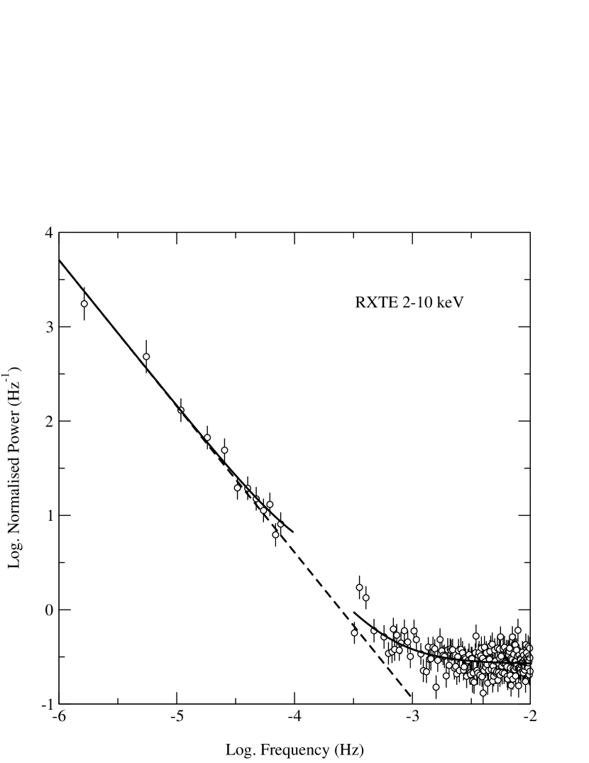
Figure 8: The 2-10 keV PSD. Fitting of the low and high frequency portions of the PSD together with a power law gives a good fit, with a slope of $\alpha=1.55^{+0.10}_{-0.06}$ and a normalization of $4.0\pm 0.6$ Hz^-1. There are no clear features such as spectral breaks or periodicities in the PSD, although there is some structure especially in the high frequency PSD, with a possible excess of power at $\sim 10^{-3.5}$ Hz

5.1 Method of calculation

The RXTE light curve of NGC 7469 is unevenly sampled and so the estimation of the power spectrum is not trivial. Here we estimate the overall power spectral density function of the source in two steps.

Firstly, we used the 16-sec binned light curve to compute the high frequency PSD. Although the light curve is not evenly sampled there are 230 parts of it with length between 1000 and $\sim 4000$ sec with no gaps in them. Therefore, we can estimate the PSD for each part and then average the resulting spectra to get a good estimation of the PSD at high frequencies. For each part we computed the periodogram using the equation,

$$\hat{I}(\nu_{j})=\frac{(\Delta t/N)\{\sum_{i=1}^{N}[x(t_{i})-\bar{x}]e^{-i2\pi\nu_{j}t_{i}}\}^{2}}{\bar{x}^{2}},$$ (1)

where: $\Delta t=16$ sec, $\nu_{j}=j/(N\Delta t)$, $j=1,2,\ldots,N/2$, and $\bar{x}$ is the mean count rate of each part. The periodogram, as defined by equation (1), is normalized to the mean count rate square and has units of $Hz^{-1}$. With this normalization, integration over positive frequencies yields half of the light curve’s relative variance. This normalization is necessary for the comparison between PSD in different energy bands.

Since the 230 parts of the light curve do not have the same length, the frequencies at which their periodograms are computed are not exactly the same. To combine them, we sorted them in order of increasing frequency, calculated their logarithm, grouped them into bins of $20$ and computed their average value at each bin. These are our final estimates of the logarithmic PSD at the geometric mean frequency of each bin (Papadakis & Lawrence 1993a).

To estimate the low frequency PSD we used the 5760s binned light curves. The use of the approximate RXTE orbital period as the bin size results in an evenly sampled light curve with very few missing points (74 out of 480, $\sim 15$% of the total). Note that these points are randomly distributed over the whole light curve, with no more than two points in a row missing. We accounted for them using linear interpolation between the two bins adjacent to the gaps, adding appropriate Poisson noise. We used equation (1) to compute the periodogram for the 5760 sec binned light curve. As above with the high frequency PSD, we computed the logarithm of the periodogram and averaged it in groups of size 20 (Papadakis & Lawrence 1993a).

Aside from the interpolation, another potential problem with the binning process is that, because the original 16s light curve also has gaps, the binning process results in data points with different exposure times. Therefore, the mean count rate at each bin is the result of averaging the signal over segments of different length at each bin. Furthermore, the location of the segment within each bin will not be the same for all bins - therefore, although we accept the average count rate at each bin as representative of the source count rate at the center of the bin, in some cases it will actually correspond to a time point other than the bin center. Consequently, strictly speaking, the 5760 sec binned light curve is not a random realization of the parent, source process and the binning may alter the light curve’s properties. We believe, however, that neither the interpolation nor the binning process will have a significant effect on our results. The source PSD is rather steep with $\alpha>1.5$ as shown by the high frequency PSD alone. Both the interpolation and the binning effect the highest frequencies most, where there is less power, and we therefore do not believe these effects will bias our results severely. Note that the best fitting slope of the PSD is mainly determined by the low frequency points. Furthermore, the effects of binning and interpolation should have the same affect on the PSD regardless of the energy range considered, and therefore our comparison of PSDs in different energy bands discussed below will not be affected.

5.2 2-10 keV PSD

Fig. 8 shows the PSD in the 2-10 keV band calculated by this method. Several things are apparent from this. First, there are no obvious “features” in the PSD, such as a low frequency knee or high frequency break. Neither are there any clear periodicities evident. We have used standard $\chi^{2}$ statistics to fit different models to the spectrum, evaluating the 68 per cent confidence regions for the model parameters using the prescription of Lampton, Margon & Bowyer (1976). The first model was a power law plus a constant of the form:

$$P(\nu)=A(10^{4}\nu)^{-\alpha}+C,$$ (2)

where: $A$ is the amplitude (in Hz^-1) at $10^{4}$ Hz, $\alpha$ is the slope and $C$ is a constant, which represents the constant Poisson power level. Rather than letting $C$ be free during the model fitting, we fixed its value to the expected noise power level. This matches the apparent noise power of the data very well indeed, as can be seen at high frequencies. This model was fitted to both the low and high frequency PSD of the source, allowing the slope and the amplitude to be different for the two parts of PSD. The results are listed in Table 3. A power law is a good fit to both spectra and the two spectra give consistent indices and amplitudes within the errors.

We also fitted this model to the combined low and high frequency power spectra, with the results shown in Table 4. The power law index of $\alpha=1.55^{+0.10}_{-0.06}$ (Table 4) is very similar to the typical value inferred by Lawrence & Papadakis (1993) from the analysis of EXOSAT data of a few Seyfert 1 galaxies. While the fit is formally acceptable, the PSD does seem to show some structure, especially at high frequencies. One interpretation of this is that there is a “QPO”–like feature at $\sim 10^{-3.5}$ Hz. If we add a Gaussian to the power law model we find a $\chi^{2}$ of 546/571, a reduction of 45.5 for 3 dof. This is formally of very high significance based on the F-test ($>99.9$ per cent confidence). The slope and amplitude do not change much ($\alpha=1.59$ and $A=4.1$ cf. Table 4), and the centroid of the “QPO” is: $\sim 3.8\times 10^{-4}$ Hz, the width (sigma) is: $\sim 2.2\times 10^{-5}$ Hz, and the amplitude $\sim 0.7$ Hz^-1. Despite the high significance, we are cautious about claiming the detection of a “QPO” in NGC 7469 for several reasons. First, the feature is very close to the frequency gap between the low and high frequency PSD, meaning we cannot determine the shape of the feature, and therefore be sure that it is in fact indicative of a periodicity. The “QPO” in the 2-10 keV PSD relies on the accuracy of the lowest point in the high frequency PSD. It is therefore difficult to know whether the poor fit – or the improvement when the gaussian is included – is due to some kind of continuum feature or break. We note that the PSD of Cyg X-1 shows high frequency structure also (Nowak et al. 1999) and we may simply be misinterpreting this as some kind of quasi-periodic signal.

The changes in RMS variability parameter shown in Fig. 4 imply that there is some change in the PSD with time, as the RMS represents an integral of the PSD over the frequency ranges sampled by the relevant light curve portion. For the daily calculations (Fig. 4 and Fig. 5) the RMS should represent approximately the integral of the PSD above a frequency of $\sim 10^{-5}$ Hz. This could represent either a change in the shape of the PSD, a change in its normalization or some combination of the two. We have investigated this by calculating the PSD as a function of time. To sample sufficient variability to provide decent constraints, we were only able to calculate the PSD every 3 days, and characterized this as a power law. Unfortunately this does not able us to distinguish unambiguously the origin of the changes in the PDS shape during the UV “dips”. When the shape (slope) is held constant at the mean value, however, the normalization shows clear changes, consistent with the changes in RMS variability parameter seen in Fig. 4. We cannot rule out the alternative of a change of shape, however.

5.3 PSD as a function of energy

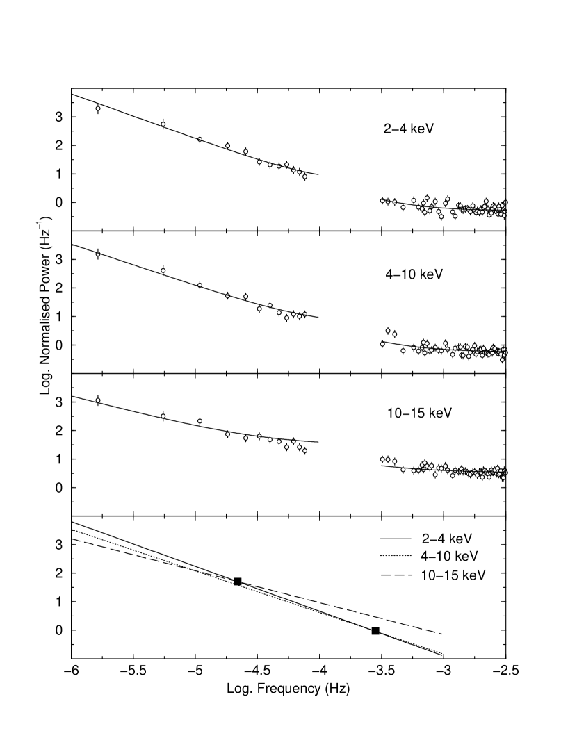
Figure 9: The top three panels show the power spectral density in the 3 different energy bands. They have been fitted with a power law model with a fixed constant representing the Poisson noise (solid lines). Note that the low and high frequency PSDs have different Poisson noise levels, however. The dashed lines show the power law only. The PSD shows a “hardening” as a function of energy, with the 10-15 keV PSD being significantly flatter than that at lower energies (see also Table 4). There is also some “structure” in the high frequency PSD, especially visible in the higher energy bands which can be fitted, albeit not uniquely with a “QPO”-like feature. The best-fit power law models for the power density spectra are shown in the bottom panel. This shows that The low energy PSD shows most power on the longest time scales, but that the opposite is true at high frequencies. The crossover point seems to be around $10^{-5}$ Hz or around 1d.

We have calculated the PSD in the 3 narrow energy bands (Fig. 1) of 2-4, 4-10, 10-15 keV by the same method as the 2-10 keV PSD. The results are shown in Fig. 9. The results of fitting the high and low frequency portions separately are also shown in Table 3. A good fit is obtained to all the spectra. The low and high frequency slopes are consistent within the errors for each individual energy band. In the 4-10 and 10-15 keV cases, however, the spectra show a systematically higher normalization in the high frequency spectra. Such an effect could be observed if there is a high frequency break in the PSD (e.g. Nowak & Chiang 2000). This break would have to occur above $10^{-4}$ Hz but it is not clearly observed in the high frequency PSD. This leaves the rather unlikely possibility that the break occurs precisely in the gap between the two PSDs. It seems equally unlikely that the PSD shows a “step” in power in this gap, maintaining (approximately) the same slope. It seems more likely that this apparent discrepancy in normalization is due to the structure or feature previously noted in the 2-10 keV PSD. Indeed visual inspection of the PSDs show that the strength of this “feature” increases with energy band.

Whatever the nature of the structure in the high frequency power spectrum it is clear from our analysis that the PSD flattens (or “hardens” to use a term borrowed from the energy spectra) as a function of energy. This is most clearly demonstrated when the low and high frequency PSDs are fitted jointly, with the results for a power law model shown in Table 4. The slope steepens from $\alpha=1.57^{+0.10}_{-0.08}$ in the 2-4 keV band to $\alpha=1.12^{+0.10}_{-0.08}$ in the 10-15 keV band. The best fit 4-10 keV PSD slope lies between the two but is formally consistent with the 2-4 keV, though inconsistent with the 10-15 keV slope. The normalizations of all three PSDs (at $10^{-4}$ Hz) are all consistent within the errors.

Despite the apparent structure at high frequencies, the fits are formally acceptable at $<90$ per cent confidence, with no clear evidence for high or low energy breaks. Although the power law is probably only a crude parameterization of a more complex form, this very clearly shows there are differences in the PSDs, and the difference is in the sense that the high frequency power spectrum shows more power at high energies. As the PSDs are normalized correctly, Fig. 9, also shows that the opposite is true at low frequencies, i.e. that there is more power on long time scales at softer energies. This is demonstrated best by the bottom panel of Fig. 9, which shows the best-fit power law models for the 3 PSDs. There appears to be a “pivot” point just above $10^{-5}$ Hz where the normalized power is roughly equal. The soft band has more power below this frequency, and the hard band more above. This behavior is similar to that seen in Cyg X-1 (Nowak et al. 1999) and has strong implications for the emission mechanisms.

6 DISCUSSION

We have presented a detailed temporal analysis of the 30d RXTE observation of NGC 7469, which was simultaneous with IUE. Strong variability was observed in all X-ray bands, with the variability amplitude observed over the whole observation being a decreasing function of energy. The variability amplitude calculated on daily time scales is similar in all energy bands, however, and shows significant changes, indicating non-stationarity. The changes are such that the most pronounced variability occurs when the X-ray spectrum is hardest and the UV flux weakest. The UV flux is positively correlated with the spectral softness ratio, and the cross-correlation shows a strong peak at zero lag, constraining the lag to be less than $\sim 8.5$ hours. The softness ratio changes are more rapid than those in the UV, however. The autocorrelation functions are very similar in the 2-4, 4-10 and 10-15 keV bands, all showing a sharp peak with FWHM of about 0.5d and broader “wings” with FWHM $\sim 5$d, reaching zero at a time scale of $\sim 4$d. The cross-correlations show a strong peak at zero lag, but are asymmetric, towards the side where the hard X-rays lag. They can be interpreted as having the same two components as the ACFs, but with the 5d FWHM component being delayed by several tenths of a day, in the sense that the soft X-ray variations lead those in the hard. The 2-10 power density spectrum shows no low frequency turnover or high frequency break. There is marginal evidence for a feature at a frequency of $3.8\times 10^{-4}$ Hz, but this may simply be due to structure or complexity in the high frequency PSD. The most striking result of the PSD analysis is that the 10-15 keV PSD is clearly flatter than the 2-4 and 4-10 keV PSD. In other words the PSD flattens or “hardens” as a function of energy. We now discuss these results in terms of the models for NGC 7469 and AGN in general.

6.1 Thermal Comptonization models

Considerable evidence is emerging that the dominant radiation mechanism producing X-rays in AGN is thermal Comptonization. The copious optical/UV radiation field is thought to act as the seed photons, which are upscattered by a corona of very hot plasma with temperatures of several hundred keV. As mentioned in the introduction, such observations fit the X-ray spectra of AGN well. Variability data also support such an interpretation. In the simplest such models, we expect to see correlated variations in the optical/UV seed and the X-rays, perhaps with a time lag in the sense that variations in the lower energy emission precede those at higher energies. Correlations between the UV and X-ray have have been observed in some cases (Clavel et al. 1992; Edelson et al. 1996). Strong correlations have also been observed between the UV and EUV emission (Marshall et al. 1997) and between the EUV and the X-ray emission (Uttley et al. 2000), and a time lag has been claimed in one case (Chiang et al. 2000). Other observations have shown much less clear behavior both in terms of the correlations and the lag (Done et al. 1990; Maoz et al. 2000; Edelson et al 2000), including those of NGC 7469 (N98).

In a realistic corona a simple correlation plus lag is not necessarily expected, however. As the UV seed flux cools the corona, this can change the coronal properties and affect the X-ray spectral shape (e.g. Pietrini & Krolik 1995; Haardt, Maraschi & Ghisselini 1997; Zdziarski, Lubinski & Smith 1999). Specifically, increases in the UV seed should result in a softer X-ray spectrum. Indeed the observation of such behavior, including in NGC 7469, provides arguably the strongest evidence for the Comptonization hypothesis (N2K; Petrucci et al. 2000). These spectral changes can, however, have an important effect on the flux as measured in a specific, narrow band, confusing any correlation (N2K). In terms of the lags, Kazanas et al. (1997) have argued that in an extended corona, covering several decades in radius, the most rapid variations at all energy bands are dominated by photons scattering close to the central source and corresponding to single scatterings. In this case, we expect the short time scale variations to exhibit only very small time lags across different energy bands. On the other hand, the longer time scales sample photons that have suffered multiple scatterings as well. Here the time lags will be revealed clearly only in the cross-spectrum, as the lags should be most prominent in the long time scale variations (e.g. Miyamoto et al 1988, 1992). We would, however, expect a smaller variability amplitude at high energies due to the “washing out” of the variability in the extended region.

Our detailed variability analysis broadly supports the thermal Comptonization model just outlined. First, at least on long time scales, we do observe a higher variability amplitude in soft X-rays than in the hard band. This is also seen in other sources (e.g. Nandra et al. 1997; Markowitz & Edelson 2000). We also confirm the correlation of the UV seed photons with the X-ray spectrum, predicted by Comptonization. Cross-correlation analysis of the UV and the softness ratio limit the time lag to be very short – less than $\sim 8$ hours. We note and discuss later that there appear to be variations in the ratio on time scales even shorter than variations in the supposed seed photons, however. This may complicate the lag error analysis and indeed as the UV does not show clear variations on time scales as short as 8 hours, this limit may be underestimated. It is clear, though, that the corona responds very rapidly to changes in the UV, implying that it is rather compact and close to the source of the seed photons.

In addition to delays between the seed photons and the X-rays, we also expect time delays within the Comptonized component. Although the intra-X-ray CCFs are peaked at zero, they are skewed towards lags in the sense that the soft X-ray variations precede those at harder energies. This is consistent with the idea that the harder photons “diffusing” through the Comptonizing medium and emerging from larger radii. Naive fitting of the CCFs suggest that they can be deconvolved into a narrow peak with zero lag and a broader component which is delayed by $\sim 0.5d$. If the delay is due to light travel time effects, it implies a very large corona (e.g. Hua et al. 1997; Kazanas et al. 1997) corresponding to a size of $\sim 1000M^{-1}_{7}\ R_{\rm g}$ where $M_{7}$ is the black hole mass in units of $10^{7}$$\rm\thinspace M_{\odot}$ (cf. the estimate for NGC 7469 of $8\times 10^{6}$ $\rm\thinspace M_{\odot}$; Collier et al. 1998). Note that such a large size is not necessarily inconsistent with the rapid variability or the peak of the CCFs at zero lag, as this can in principle originate in the innermost parts of the corona after single scatterings. Another possibility is that the delays are not due to a light travel time or the Comptonization process but, for example, to an instability time scale in the accretion disk. The skewing of the CCF implies an instability or flare propagating inwards on a time scale of $\sim 1d$, first affecting the softer X-rays and then inducing variability in the hard X-rays. In this scenario, the sharp peaks in the CCFs should correspond to the fact that the X-ray emitting flares respond to the UV seed variations with no delays (i.e. an optically thin corona) as the very small lag between the UV and the softness ratio indicates.

6.2 Rapid variability: a coronal origin?

Despite the broad support which our variability analysis affords the Comptonization model, it is becoming clear that there is a variability process distinct from the apparent Compton seed (i.e. the observed UV). N98 had already noted that rapid variations in the 2-10 keV X-ray flux were observed which were not present in the UV. We have also shown that there are rapid changes in the X-ray spectrum which occur faster than changes in the supposed seed. This implies that, if the UV are indeed the seed photons, they cannot be solely responsible either for the flux variability in the X-rays, or the spectral variations via cooling. A potential way of explaining this is that UV acts as a surrogate for the “true” seed photons, the EUV, which might show (unobserved) variations even more rapid than the X-rays. Our observation of a “hardening” of the PSD as a function of energy appears to rule this out, however. Wherever the seed photons originate, once they are up scattered we expect the high frequency variability to be less at high energies. We therefore conclude that there must be a mechanism unrelated to the seed photons that dominates the variability on time scales of less than about one day. We note with great interest that the same behavior has been observed for Cyg X-1 by Nowak et al. (1999), albeit on a time scale $\sim 10^{6}$ times shorter. Our conclusion is the same as theirs, that the fast variability most likely something to do with the process which heats the corona. For example, the magnetic flare model of Poutanen & Fabian (1999) predicts at least that the high frequency power spectrum should be similar at all energies.

Assuming that the X-rays are indeed produced by Compton upscattering, it seems highly unlikely that this “hardening” of the PSD can be produced in a model where the X-rays are produced in a single, coherent region. In such a scenario, any changes in the seed photons would affect the PSD in the opposite way to that observed. Indeed, this hardening appears to rule out the possibility even of an inhomogeneous, extended corona as proposed by Kazanas et al. (1997). In this model the zero lag peaks in the CCFs are due to contributions from single scattered photons in the central regions of the corona, from which the rapid variability arises. At the very least we would then expect to see the same amplitude at high frequencies but much more likely the variability should be drastically reduced with the PSD rapidly steepening as a function of energy due to the “washing out” effect of multiple scatterings described above (Brainerd & Lamb 1987; Nowak & Vaughan 1996; Hua & Titarchuk 1996; Kazanas & Hua 1999). One way out of this is by hypothesizing that the extended corona has a temperature gradient as well as having a density gradient, and that the hotter inner regions respond to a very rapidly variable seed source which we do not observed (e.g. the EUV). ADAF models, for example, exhibit such a gradient, with the temperature being constant out to some radius, outside which it drops as $R^{-1}$ (Narayan & Yi 1994). It seems more likely, however, that the data are indicating that the corona is patchy, consisting of “flares”. Again the flares in the inner regions should typically be hotter. They would therefore account for more of the high energy photons, but be more rapidly variable because of their smaller size scale. Depending on the heating mechanism, it may take time for the electron temperature to respond to changes in the heating rate and those changes also have a finite time scale associated with them. This could potentially have different effects at different energies. For example if the temperature change propagates from the inner to the outer regions in a finite time, this would produce more rapid variations in the hard flux in those inner regions. We await a detailed model that explains this flattening of the PSD with increasing photon energy.

Our interpretation is of two separate origins for the variability, one due to variations in the seed photons and another due to the coronal heating mechanism. The first dominates the variability on time scales greater than about 1 day, gives a larger amplitude in the soft X-rays and induces spectral variability by cooling the corona. The time delay involved is very short, with the CCF of the UV vs. the softness ratio being peaked at zero, but it is skewed to positive lags in a similar fashion to the intra-X-ray CCFs. The second process induces high frequency variability roughly simultaneously at all energies, but with larger amplitude at high energies. It results in intra-X-ray CCFs which are strongly peaked at zero, explaining the sharp central peak in the ACFs and CCFs. Since the rapid variability mechanism affects the harder energies more, it seems highly unlikely that the X-ray emitter is a single region, but rather consists of localized “flares”. This mechanism must also induce rapid spectral variability, because we observe changes in the X-ray hardness ratio as short as $\sim 90$ min (1 orbit) which are more rapid than the variations in the UV seed flux. Once again, this cannot be account for by invoking a more rapidly-varying EUV seed because of the hardening of the PSD. It seems reasonable for the coronal heating mechanism to induce rapid spectral variability – after all, the very process of heating would results in a spectral change.

We note that a “two-process” variability mechanism is suggested by some other observations, notably those of NGC 3516 (e.g. Maoz et al. 2000; Edelson et al. 2000) which appear to show rather similar characteristics to NGC 7469. In particular the most rapid variations in the X-rays are not observed in the optical (Maoz et al. 2000). The soft X-rays vary simultaneous with the hard X-rays, but have larger amplitude on time scales of a few days (Edelson et al. 2000). NGC 5548 also shows this behavior, with the soft X-ray/hard X-ray CCF having a peak at zero lag but being strongly skewed towards positive lags (Chiang et al. 2000). Chiang et al. also show evidence for an explicit time delay in this source, with the EUV emission leading the X-rays by $\sim 30ks$, rather similar to the “lag” time scale inferred here. A prediction of our model is that the cross-spectrum should show time lags at long time scales which will be smaller on short time scales, as seen in Cyg X-1 (Miyamoto et al. 1992).

Note that, as discussed by N2K, the longer-timescale variations induced by the seed photons need not be intrinsic to the material producing them (e.g. the accretion disk). Energetically it is possible that the optical/UV variations on time scales of a few days are due to reprocessing of soft X-ray photons. This is consistent with the fact that we observe changes in the hardness ratio faster than those in the UV flux – these variations being smoothed out by an extended reprocessor, and the observation of time lags within the UV and optical (Wanders et al. 1997; Collier et al. 1998). The reprocessed seed variations would then cool the corona, in turn changing the reprocessed flux and back again, in exactly the kind of “feedback” mechanism envisaged by Haardt & Maraschi (1991, 1993). We favor such a mechanism for the origin of the X-ray and variable UV radiation in NGC 7469 and other AGN, with the added provisos that the corona is patchy (Haardt et al. 1994; Stern et al. 1995) and the heating should occur in rapid, localized “bursts” (which may amount to the same thing). These bursts or flares cannot be static, and each must either have a different intrinsic properties (e.g. $\tau$, $kT$, geometry) or different evolution of those properties. Possibilities include that mentioned above, that the inner regions are hotter and more rapidly variable, or that the inner regions have roughly the same initial properties, but evolve more rapidly than the inner region.

6.3 Features in the PSD

We observe no clear features in the PSD of NGC 7469, such as the low frequency “knee” (Papadakis & McHardy 1995; Edelson & Nandra 1999) or high frequency “break” (Nowak & Chiang 1999). There is some structure in the high frequency PSD which can be modeled as a “QPO” on a timescale of approximately 2500s. This is similar to the time scales of QPO which have been reported from some EXOSAT observations (Papadakis & Lawrence 1993b; Papadakis & Lawrence 1995). We are cautious about such an interpretation here, however. The shape of the QPO cannot be determined as it is very close to the gap between the low– and high–frequency PSDs and it could simply be that the high frequency PSD is “noisy” and not well fit by a simple power law. This is also seen in Cyg X-1 (Nowak et al. 1999) and has been interpreted as there being a more complex power spectral form (e.g. Nowak 2000). We await better data, which can be obtained with, e.g. XMM, on the short-medium time scales before drawing firm conclusions about NGC 7469 or other AGN.

6.4 Rapid variability of the PSD

A final intriguing result from the X-ray variability of NGC 7469 is the apparent increase in the RMS variability parameter when the UV flux is weakest and the X-ray spectrum the hardest. The behavior of this individual object contrasts with that when comparing objects where sources with flat spectra are less variable, at least on $\sim d$ time scales (e.g. Green et al. 1993; Turner et al. 1999). The reason for the behavior in NGC 7469 is not clear at this point, but it may be related to some form of instability in the corona. For example, as the spectrum hardens it may reach a critical point at which electron-positron pair production becomes important, inducing additional variability. Naively, however, we might expect this to increase the optical depth, smoothing out rapid variability, however. We have hypothesized above that the hotter parts of the corona occur closer in, in order to explain the “hardening” of the PSD. If this is indeed the case, then the source should be most rapidly variable (in a normalized sense) when the spectrum is hardest, and therefore the flux dominated by the innermost, hottest and most rapidly variable regions. The increase in RMS is also consistent with an increase in the normalization of the PSD (although we are not able to rule out the possibility that the shape changes). In the general context of shot noise models, with flares happening randomly, the normalized PSD amplitude can change in two ways: 1) the mean rate of flares per unit time changes or 2) the flare shape changes in the sense that flares last shorter or longer. The latter seems more consistent with the observation of an increased RMS when the flux is weak. Whatever the origin of these phenomena, it is clear that variability still has much to tell us about both the radiation mechanism and the dissipation process that causes active galaxies to emit X-rays.

Table 1: Variability parameters

Band	$\overline{F}$	$\sigma_{\rm F}$	$\sigma^{2}_{\rm RMS}$ (5760s)	$\sigma^{2}_{\rm RMS}$ (16s)
2-10	8.64	1.83	$2.55\pm 0.16$	$2.78\pm 0.03$
2-4	4.26	1.09	$2.99\pm 0.19$	$3.26\pm 0.05$
4-10	4.23	1.04	$2.22\pm 0.14$	$2.44\pm 0.05$
10-15	1.22	0.59	$1.81\pm 0.16$	$2.43\pm 0.19$

Note. — $\overline{F}$ is the mean flux in ct s^-1; $\sigma_{\rm F}$ is the square root of the variance of the light curve (ct s^-1). $\sigma^{2}_{\rm RMS}$ is the excess variance in units of $10^{-2}$ (dimensionless), calculated from the 5760s light curves and 16s light curves.

Table 2: Cross-correlation results

Band	$r_{\rm 0}$ (256s)	Delay (ks)	$r_{\rm 0}$ (5760s)	Delay (ks)
2-4 keV vs. 4-10 keV	0.83	$0.7\pm 0.8$	0.85	$1.4\pm 2.0$
2-4 keV vs. 10-15 keV	0.49	$1.1\pm 1.9$	0.67	$0.6\pm 3.0$
4-10 keV vs. 10-15 keV	0.49	$0.5\pm 1.7$	0.73	$0.0\pm 2.3$
UV vs. 2-4/4-10 keV	$\cdots$	$\cdots$	0.44	$-8.1\pm 30.3$

Note. — $r_{\rm 0}$ is the correlation coefficient at zero lag. As the zero lag points have been suppressed in the X-ray/X-ray correlations, due to correlated errors, this was estimated as the average of the two adjacent bins; the delays were calculated using the method of Peterson et al. (1998).

Table 3: Results of Power Law model fitting to the Low and High frequency PSD of NGC 7469

Band	$\alpha_{low}$	Alow (Hz${}^{-1})$	$\alpha_{high}$	Ahigh (Hz${}^{-1})$	$\chi^{2}$/dof
$2-10$ keV	$1.58^{+0.16}_{-0.15}$	$3.8^{+1.1}_{-0.9}$	$1.72^{+0.39}_{-0.32}$	$5.8^{+6.2}_{-2.8}$	555.1/572
$2-4$ keV	$1.58^{+0.16}_{-0.17}$	$4.5^{+1.7}_{-1.1}$	$1.29^{+0.72}_{-0.35}$	$2.7^{+4.4}_{-1.6}$	607.4/572
$4-10$ keV	$1.57^{+0.18}_{-0.17}$	$3.3^{+1.2}_{-0.9}$	$1.99^{+0.70}_{-0.48}$	$12.7^{+25.4}_{-7.4}$	588.7/572
$10-15$ keV	$1.48^{+0.23}_{-0.22}$	$3.9^{+2.6}_{-1.8}$	$1.94^{+0.65}_{-0.48}$	$62.9^{+105.7}_{-37.7}$	560.3/572

Note. — $A$ is the normalization of the PSD at $10^{-4}$ Hz and $\alpha$ the slope. Parameters marked “low” refer to the low frequency PSD below $\sim 10^{-4}$ Hz and “high” refer to the high frequency PSD above $\sim 10^{-3.5}$ Hz

Table 4: Results of the Power Law model fitting to the combined Low+High frequency PSD of NGC 7469

Band	$\alpha$	$A$ (Hz${}^{-1})$	$\chi^{2}$/dof
$2-10$ keV	$1.55^{+0.10}_{-0.06}$	$4.0^{+0.6}_{-0.6}$	591.5/574
$2-4$ keV	$1.57^{+0.10}_{-0.08}$	$4.7^{+0.8}_{-0.8}$	608.2/574
$4-10$ keV	$1.46^{+0.07}_{-0.08}$	$4.2^{+0.7}_{-0.6}$	593.6/574
$10-15$ keV	$1.12^{+0.10}_{-0.08}$	$9.4^{+1.9}_{-1.9}$	579.2/574

Appendix A Effects of residual background variations on the power spectra

As the ACF, CCF and PSD techniques is rather sensitive, particularly to periodic signals, our results could be strongly affected by any residual uncertainty in the background subtraction. We now investigate such affects using both a 4d observation of a “blank sky” pointing and the high energy data for NGC 7469, which are more dominated by background.

A.1 The 4d background

Figure 10: (left panels) Low frequency periodograms of the 4 day background observation in (top to bottom) 2-4, 4-10, 10-15 and 15-24 keV bands. The dashed line shows the 95% confidence limit assuming the periodogram consists only of the expected Poisson noise, with no signal. A significant signal is observed on a time scale of $\sim 1d$ in the 15-24 keV light curve, which is also visible but much less prominent in the 2-4 keV light curve. (right panels) high frequency periodograms in the same bands. Only one peak is seen above this level, in the 10-15 keV periodogram, and this is at a frequency deep within the noise of the NGC 7469 PSD.

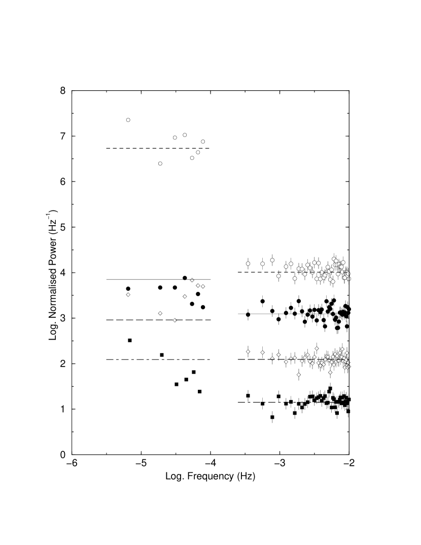
Figure 11: PSD of the 4 day background observation in 4 bands. Open circles are the 15-24 keV power spectrum, filled circles are the 10-15 keV, open diamonds the 4-10 keV, and filled squares the 2-4 keV. Short dashed line, solid line, long-dashed line and dotted-dashed line are the expected Poisson noise level in each band.

As part of the development of the background model, RXTE makes observations of several points in the sky which are free from bright sources - so-called “blank sky” pointing. One such observation was made near-continuously for $\sim 4$d, which was intended to identify medium-timescale trends and periodicities in the background. Though shorter, this dataset is the blank sky pointing which most closely resembles our NGC 7469 dataset, and can be used to search for systematic effects which might bias our results. We applied the background subtraction model to this dataset in the same way as for NGC 7469, and extracted light curves (using a bin of size 16 and 5760 sec) in the same four energy bands. We used these light curves and the same method as with the NGC 7469 data to estimate the power spectrum at high and low frequencies respectively. The unbinned periodograms are shown in Fig. 10.

Under the hypothesis that the background model describes the observed background properly their power spectrum should be constant and equal to the constant Poisson noise power level ($\Delta t\times\sigma^{2}$, where $\sigma$ is the variance of the light curve). Note that the means of the background-subtracted light curves are not zero, with the 2-4, 4-10, 10-15 and 15-24 keV light curves showing offsets from zero relative to the predicted background of 3.5, 3.7, 1.5 and -0.2 per cent levels respectively. These contributions, and the reduction in them with increasing energy, is consistent with a positive diffuse background fluctuation in the direction of the background pointing, which should be constant and will not affect the power spectra. When we subtract off the mean value from the light curves a residual constant component will be removed. We note that this may have a small effect on our calculation of the RMS values, due to a small inaccuracy in the calculation of the mean, but this is smaller than the associated statistical error (at least for the 5760s light curves) and so can be ignored. The periodograms in Fig. 10 have been divided by the expected Poisson power level, in which case the points should have a $\chi^{2}$ distribution with two degrees of freedom (Papadakis & Lawrence 1993a). Normalized in this way, we can calculate a confidence level from the periodogram to exceed a certain value, and the 95 per cent confidence limit (accounting for the number of points) is shown as the dashed line in the Figure. Examining first the high frequency periodogram (right panels of Fig. 10) we see that, although there are a few spikes only one exceeds the 95 per cent confidence level. This is in the 10-15 keV light curve at a frequency $\sim 2.3\times 10^{-2}$, well into the noise of the NGC 7469 PSD (c.f. Fig. 8). We conclude that residual errors in the background subtraction will not affect the high frequency PSD. As for the low frequencies (left panels of Fig. 10), the 15-24 keV periodogram shows a sharp peak at $\sim 10^{-5}$s, which is also present, but at a much lower level, in the 2-4 keV band. This probably represents a daily periodicity, which we discuss further below.

Figure 12: ACF of the 15-24 keV light curve of NGC 7469, calculated by the interpolation method. This shows peaks every day which are almost certainly due to residual background.

Fig. 11 shows the combined background power spectra, this time normalized to the mean squared as the NGC 7469 data, in log space and with the high frequency PSD binned like that of NGC 7469. They are flat and consistent with the expected power level. We find no systematic excess of power at high frequencies for the hard X-ray light curve, which might account for the “hardening” of the PSD just noted. Neither do we find a clear feature at $\times 10^{-3.5}$ Hz where an excess is observed in the NGC 7469 PSD. Furthermore we find no systematic differences between the four power spectra. Although we note that this 4d PSD is not as high quality as the 30d PSDs we derived for NGC 7469, this analysis indicated that our conclusion for NGC 7469 are robust and secure.

A.2 The high energy NGC 7469 data

The PCA team (Jahoda, priv. comm) have presented evidence for a daily periodicity like that seen in Fig. 10 in the 30-70 keV light curves of various datasets, attributed to residual errors in the background. In our analysis of NGC 7469, we had initially hoped to extend our analysis above 15 keV, where the effects of PSD hardening would have been much more pronounced. We found, however, that the 15-24 keV bands was strongly affected by this daily periodicity.

Figure 13: Unbinned low frequency PSD of NGC 7469 in four energy bands (top to bottom): 2-4 keV, 4-10 keV, 10-15 keV and 15-24 keV, plotted in linear space. The 15-24 keV PSD shows a very clear periodicity on a timescale of 1 day, and associated harmonics. This periodicity is due to daily variations in the background which have not been modeled correctly. The periodicity is very much weaker in the other bands, and has a negligible effect on them.

Fig. 12 shows the autocorrelation function of the NGC 7469 light curve in the 15-24 keV band. This clearly shows very strong, daily peaks. There is very little signal in the ACF other than this daily variations, which show that they dominate the variability in this band. Note that the ACFs in the lower energy bands do not show a strong signal on this time scale, with the source signal dominating (Fig. 6). Nonetheless, even if present at a lower level in the in the other energy bands they could bias our estimate of the PSD and introduce spurious signals in the CCFs. We do not believe this is a strong effect, however. Fig. 13 shows the unbinned, low frequency periodogram in linear space for the four bands between 2 and 25 keV. As expected, the 15-24 keV plot shows a very strong peak at the daily time scale, and also strong harmonics. The other periodograms also show peaks but these are much smaller and will not significantly affect our estimates of the power spectra. We have tested this by removing the data points at the daily periodicity and the two harmonics from the lower energy periodograms, binning them and comparing to the binned PSDs in Fig. 9. No significant difference is observed, leaving us confident that background effects do not bias our results. We particularly note that there are no significant biases as a function of energy that would indicate problems with our conclusion of the PSD hardening.

References

- (1)
- (2) Abramowicz, M.A., Bao, G., Lanza, A., Zhang, X.-H., 1991, A&A, 245, 454
- (3) Alexander, T., 1997, in “Astronomical Time Series”, D. Maoz, A. Sternberg, E. Leibowitz, Eds, Kluwer, Dordrecht, p. 163
- (4) Bao, G., Abramowicz, M.A., 1996, ApJ, 465, 646
- (5) Belloni, T., Hasinger, G., 1990, A&A, 230, 103
- (6) Brainerd, J., Lamb, F.K., 1987, ApJ, 317, L33
- (7) Chiang, J., et al., 2000, ApJ, 528, 292
- (8) Clavel, J., et al., 1992, ApJ, 393, 113
- (9) Collier, S., et al., 1998, ApJ, 500, 162
- (10) Done, C., Ward, M.J., Fabian, A.C., Kunieda, H., Tsuruta, S., Lawrence, A., Smith, M.G., Wamsteker, W., 1990, MNRAS, 243, 713
- (11) Edelson, R.A., et al., 2000, ApJ, 534, 180
- (12) Edelson, R.A., Krolik, J.H., 1987, ApJ, 333, 646
- (13) Edelson, R.A., Nandra, K., 1999, ApJ, 514, 682
- (14) Edelson, R.A., et al., 1996, ApJ, 470, 364
- (15) Gaskell, C.M., Peterson, B.M., 1986, ApJS, 65, 1
- (16) Gondek, D., Zdziarski, A.A., Johnson, W.N., George, I.M., McNaron-Brown, K., Magdziarz, P., Smith, D., Gruber, D.E., 1996, MNRAS, 282, 646
- (17) Green, A.R., McHardy, I.M., Lehto, H.J., 1993, MNRAS, 265, 664
- (18) Haardt, F., Maraschi, L., 1991, ApJ, 380, 51
- (19) Haardt, F., Maraschi, L., 1993, ApJ, 413, 507
- (20) Haardt, F., Maraschi, L., Ghisellini, G., 1994, ApJ, 432, L95
- (21) Haardt, F., Maraschi, L., Ghisellini, G., 1997, ApJ, 476, 620
- (22) Hua, X.-M., Titarchuk, L., 1996, ApJ, 469, 280
- (23) Hua, X.-M., Kazanas, D., Titarchuk, L., 1997, ApJ, 482, L57
- (24) Kazanas, D., Hua, X.-M., Titarchuk, L., 1997, ApJ, 480, 735
- (25) Kazanas, D., Hua, X.-M., 1999, ApJ, 519, 750
- (26) Jahoda, K., Swank, J.H., Giles, A.B., Stark, M.J., Strohmayer, T., Zhang, W., Morgan, E.H., 1996, EUV, X-ray and Gamma-ray Instrumentation for Space Astronomy VII, O. H. W. Siegmund and M. A. Grummin, Eds., SPIE 2808, p. 59
- (27) Kriss, G.A., Peterson, B.M., Crenshaw, D.M, Zheng, W., 2000, ApJ, 535, 58
- (28) Lawrence, A., Papadakis, I., 1993, ApJ, 414, L85
- (29) Lawrence, A., Watson, M.G., Pounds, K.A., Elvis, M., 1985, MNRAS, 217, 685
- (30) Leighly, K., Mushotzky, R.F., Yaqoob, T., Kunieda, H., Edelson, R.A., 1996, ApJ, 469, 147
- (31) Malkan, M.A., Sargent, W.L., 1982, ApJ, 254, 22
- (32) Maoz, D., Edelson, R.A., Nandra, K., 2000, AJ, 119, 119
- (33) Markowitz, A., Edelson, R.A., 2001, ApJ, in press
- (34) Marshall, H., et al., 1997, ApJ, 479, 222
- (35) McHardy, I.M., Czerny, B., 1987, Nature, 325 696
- (36) McHardy, I.M., Papadakis, I., Uttley, P., 1998, in The Active X-ray Sky: results from BeppoSAX and RXTE, L. Scarsi, H. Bradt, P. Giommi, and F. Fiore, Eds. (Amsterdam: Elsevier), p. 509
- (37) Miyamoto, S., Kitamoto, S., Mitsuda, K., Dotani, T., 1988, Nature, 336, 450
- (38) Miyamoto, S., Kitamoto, S., Iga, S., Negoro, H., Terada, K., 1992, ApJ, 391, 21L
- (39) Molendi, S., Maraschi, L., Stella, L., 1992, MNRAS, 255, 27
- (40) Narayan, R., Yi, I., 1994, ApJ, 428, L13
- (41) Nayakshin, S., Melia, F., 1997, ApJ, 490, L13
- (42) Nandra, K., et al., 1998, ApJ, 505, 594 (N98)
- (43) Nandra, K., et al., 2000, ApJ, 544, 734 (N2K)
- (44) Nandra, K., George, I.M, Mushotzky, R.F., Turner, T.J., Yaqoob, T., 1997, ApJ, 476, 70
- (45) Nandra, K., Pounds, K.A., 1994, MNRAS, 268, 405
- (46) Nowak, M., 2000, MNRAS, 318, 361
- (47) Nowak, M., Chiang, J., 2000, ApJ, 531, L13
- (48) Nowak, M.A., Vaughan, B.A., Wilms, J., Dove, J. B., Begelman, M. C., 1999, ApJ, 510, 874
- (49) Papadakis, I., Lawrence, A., 1993a, MNRAS, 261, 612
- (50) Papadakis, I., Lawrence, A., 1993b, Nature, 361, 233
- (51) Papadakis, I., Lawrence, A., 1995, MNRAS, 272, 161
- (52) Papadakis, I., McHardy, I.M., 1995, MNRAS, 273, 923
- (53) Peterson, B.M., Wanders, I., Horne, K., Collier, S., Alexander, T., Kaspi, S., Maoz, D., 1998, PASP, 110, 660
- (54) Petrucci, P.-O. et al., 2000, ApJ, 540, 131
- (55) Pietrini, P., Krolik, J.H., 1995, ApJ, 447, 526
- (56) Poutanen, J., Fabian, A.C., 1999, MNRAS, 306, L31
- (57) Shapiro, S.L., Lightman, A.P., Eardley, D.M., 1976, ApJ, 204, 187
- (58) Stern, B.E., Poutanen, J., Svensson, R., Sikora, M., Begelman, M.C., 1995, ApJ, 449, L13
- (59) Sunyaev, R.A., Titarchuk, L.G., 1980, A&A, 86, 121
- (60) Turner, T.J., George, I.M., Nandra, K., Turcan, D., 1999, ApJ, 524, 667
- (61) Uttley, P., McHardy, I.M., Papadakis, I.E., Cagnoni, I., Fruscione, A., 2000, MNRAS, 312, 880
- (62) Wanders, I., et al., 1997, ApJS, 113, 69
- (63) Welsh, W.F., 1999, PASP, 111, 1347
- (64) White, R.J., Peterson, B.M., 1994, PASP, 106, 879
- (65) Wiita, P.J., Miller, H.R., Carini, M.T., Rosen, A., 1991, in Structure and Emission Properties of Accretion Disks, ed. C. Bertout et al. (Gif-sur-Yvette: Ed. Frontieres), p557
- (66) Zdziarski, A.A., Fabian, A.C., Nandra, K., Celotti, A., Rees, M.J., Done, C., Coppi, P.S., Madejski, G.M., 1994, MNRAS, 269, L55
- (67) Zdziarski, A.A., Lubinski, P., Smith, D.A., 1999, MNRAS, 303, L11
- (68)