A Richness Study of 14 Distant X-ray Clusters From the 160 Square Degree Survey

Abstract

We have measured the surface density of galaxies toward 14 X-ray-selected cluster candidates at redshifts $z\mathrel{>\kern-10.00002pt\lower 3.87495pt\hbox{$\sim$}}0.46$, and we show that they are associated with rich galaxy concentrations. These clusters, having X-ray luminosities between $L_{\rm x}(0.5-2)\sim 0.5-2.6\times 10^{44}~{}{{\rm ergs\ s}^{-1}}$, are among the most distant and luminous in our $160$ square degree $ROSAT$ PSPC cluster survey. We find that the clusters range between Abell richness classes $0-2$, and have a most probable richness class of one. We compare the richness distribution of our distant clusters to those for three samples of nearby clusters with similar X-ray luminosities. We find that the nearby and distant samples have similar richness distributions, which shows that clusters have apparently not evolved substantially in richness since redshift $z=0.5$. There is, however, a marginal tendency for the distant clusters to be slightly poorer than nearby clusters, although deeper, multicolor data for a large sample would be required to confirm this trend. We compare the distribution of distant X-ray clusters in the $L_{\rm x}$–richness plane to the distribution of optically-selected clusters from the Palomar Distant Cluster Survey. The optically-selected clusters appear overly rich for their X-ray luminosities when compared to X-ray-selected clusters. Apparently, X-ray and optical surveys do not necessarily sample identical mass concentrations at large redshifts. This may indicate the existence of a population of optically rich clusters with anomalously low X-ray emission. More likely, however, it reflects the tendency for optical surveys to select unvirialized mass concentrations, as might be expected when peering along large-scale filaments.

Accepted for publication in the Astrophysical Journal

1 Introduction

In hierarchical cosmologies, structure forms on broad mass scales from the growth of density perturbations in the early Universe. The rate at which structure grows is governed by the cosmological parameters, particularly the density parameter $\Omega_{0}$ (White & Rees 1978; Kaiser 1986). Dark matter halos on cluster mass scales grow slowly at redshifts below $z\simeq 1$ in low density, hierarchical model Universes and flat, lambda-dominated Universes, while rapid and continuous growth is expected between $z\sim 0.5$ and the present in a flat, $\Omega_{0}\simeq 1$ Universe with zero cosmological constant (Richstone, Loeb, & Turner 1992, Luppino & Gioia 1995, Eke, Cole, & Frenk 1996, Bahcall, Fan, & Cen 1997, Mathiesen & Evrard 1998, Viana & Liddle 1998).

To the extent that X-ray emission traces deep cluster potential wells, the abundance of X-ray clusters at redshifts $0.4\mathrel{<\kern-10.00002pt\lower 3.87495pt\hbox{$\sim$}}z\mathrel{<\kern-10.00002pt\lower 3.87495pt\hbox{$\sim$}}1$ should probe $\Omega_{0}$ directly and with high sensitivity. Accordingly, several X-ray-selected samples of distant clusters have been drawn from the $ROSAT$ archive to investigate this issue (e.g. Collins et al. 1997, Jones et al. 1998, Rosati et al. 1998, Vikhlinin et al. 1998a, Henry et al. 2001, Gioia et al. 2001). These surveys have yielded no evidence for evolution of cluster abundances for clusters with X-ray luminosities below $L_{\rm x}(0.5-2)\mathrel{<\kern-10.00002pt\lower 3.87495pt\hbox{$\sim$}}3\times 10^{44}~{}{{\rm ergs\ s}^{-1}}$ and redshifts below $z\sim 0.4$. However, there is a growing body of evidence for a mild but significant decrease in the abundance of the most X-ray-luminous distant clusters (Henry et al. 1992, Vikhlinin et al. 1998b).

The degree to which clusters have matured into galaxy-rich, virialized structures as a function of look-back time (redshift) likewise depends on the cosmological parameters, and is therefore an important aspect of cluster evolution (Kaiser 1986; Frenk et al. 1996). However, it is difficult to select samples of clusters to study the systematic properties of cluster galaxy populations–the degree to which clusters have evolved into rich concentrations of galaxies, for example–while avoiding fatal selection biases. Because the optical detectability of distant clusters is itself coupled to their degree of galaxy concentration, optically-selected samples are not ideally suited to such studies. On the other hand, X-ray-selected clusters are largely unbiased with regard to the galaxy population, and are therefore suited to studies of cluster galaxy evolution. Furthermore, the existence of reasonably well-defined relationships between X-ray luminosity, temperature, and mass (Evrard, Metzler, & Navarro 1996, Mushotzky & Scharf 1997, Markevitch 1998) make it possible to use X-ray flux-limited samples of clusters in the nearby and distant Universe to determine the degree to which the galaxy populations have settled into their cluster potential wells as function of time and cluster mass. One measure of this process is cluster richness (Yee and Lopez-Cruz 1999).

In this paper we examine the richness distribution (i.e. the net number of galaxies encircled by the Abell radius within two magnitudes of the third brightest galaxy) for 14 of the 28 most distant clusters found in our $ROSAT$ 160 square degree cluster survey (Vikhlinin et al. 1998a). We compare our cluster richnesses to those of nearby clusters with similar X-ray selection criteria, and to those for distant, optically-selected clusters (e.g. Bower et al. 1994, Holden et al. 1997, Couch et al 1991, Postman et al. 1996), and we discuss our results in the context of cluster evolution.

2 Observations

The clusters were discovered using the X-ray selection function described in Vikhlinin et al. (1998a). Of the two to three dozen cluster candidates beyond $z\mathrel{>\kern-10.00002pt\lower 3.87495pt\hbox{$\sim$}}0.45$ discovered in our survey, the 14 for which we have the best optical data are listed in Table 1. The spectroscopic redshifts measured for the brightest one to three galaxies nearest the X-ray centroid are taken from Mullis et al. (2001, in preparation). We obtained R-band Harris filter images of candidate clusters with the 1.2 m telescope of the F.L. Whipple Observatory, the 1 m Las Campanis telescope, the Danish 1.5 m telescope, and the 3.6 m telescope at La Silla during many observing runs from June 1995 to February 1999. The optical images were originally obtained to determine whether the extended X-ray sources correspond to optical galaxy concentrations, and to measure photometric redshifts for the clusters. Several CCD cameras were used over the course of the survey. Exposure times ranged from 10 min to over an hour, and seeing was typically 1.3 arcsec. The fields of view were 10.6 arcmin, 13.3 arcmin, 23 arcmin, and 5.5 arcmin for the 1.2 m, 1.5 m, 1 m, and 3.6 m telescopes respectively. For reference, 2.3 arcmin corresponds to a linear size of 1 Mpc at $z=0.5$ for ${\rm H}_{0}=50~{}{\rm km}~{}{\rm s}^{-1}~{}{\rm Mpc}^{-1}$ and $q_{0}=0.5$, which is assumed throughout this paper. Deep images of Cl 0529-5848 and Cl 1311-0551 were taken with the EFOSC camera on the 3.6 m telescope at La Silla. These images provided a deep measurement of the galaxy luminosity function within a 1 Mpc radius for the two clusters. We used the average of these luminosity functions to calculate magnitude depth incompleteness corrections when estimating richnesses for the remaining clusters. All CCD image frames were de-biased, overclock-corrected, flat-fielded, and combined using IRAF routines to form the science images for each cluster.

3 Galaxy Selection and Photometry

The galaxies were selected for the analyses described below as follows. Using a wavelet detection routine, we determined the locations of all sources on the science CCD frames. We measured the full width at half maximum (FWHM) in right ascension and declination of each object, and rejected all point-like objects and bright foreground stars and galaxies. We measured instrumental magnitudes for each galaxy using 3 arcsec and 6 arcsec diameter apertures, which correspond to 22 and 44 kpc linear diameters at $z=0.5$.

We then ranked the galaxies by magnitude relative to the brightest galaxy nearest the X-ray centroid. The brightest cluster galaxy and one or two companions were used to determine the spectroscopic redshift of the cluster (Mullis et al. 2001, in preparation). Galaxies within the Abell radius brighter than $m_{3}+2$, where $m_{3}$ is the third brightest galaxy magnitude, were selected from the catalog.

We counted galaxies in the magnitude-selected subsample of cluster and field galaxies within centered apertures of $0.25,~{}0.5,~{}1.0,$ and $1.5$ Mpc radius. We determined the background by averaging the counts in 20–30 apertures placed at random locations away from the cluster. The net number of cluster galaxies was estimated by subtracting the mean background counts, adjusted appropriately for area, from the counts in the cluster aperture.

We restricted our search for the third brightest cluster galaxy to a radius of 0.5 Mpc to minimize foreground galaxy contamination that can introduce errors into the richness measurements (Postman et al. 1996). Using the integrated luminosity function discussed in §6.1, we find that a half magnitude error in the counting depth can cause a $\approx 60\%$ error in the richness estimate. Errors of this magnitude can be introduced when a bright foreground galaxy is misidentified as the third brightest cluster galaxy (e.g. Postman et al. 1996). This would cause $m_{3}$ to be underestimated, which in turn would cause us to mine to erroneously shallow depths. This chain of errors would then result in erroneously small cluster richness estimates. Applying the Abell radius criterion to distant cluster fields would produce this error most of the time (e.g. Postman et al. 1996). Therefore, we mitigated this effect by selecting the third brightest galaxy within a half Mpc radius.

We determined whether we were successful at mitigating the third brightest galaxy problem by comparing our distribution of $m_{1}-m_{3}$ to the distribution in the ACO catalog. We found good agreement between the two samples. The mode for our 14 cluster sample is $m_{1}-m_{3}\approx 0.4$ magnitudes, which compares well to the ACO value of $\approx 0.35$ magnitudes. We therefore do not appear to be significantly biased in this respect. Nevertheless, using another method, we were able to circumvent this process entirely by comparing galaxy counts in nearby and distant clusters within restricted apertures and depths in §4 and §5. The analysis was done using our own routines written in IDL and FORTRAN. We compared our galaxy selection algorithm to the “SExtractor” routine and found similar results. We show an optical image, with X-ray contours superposed, of a typical richness class 0 cluster discovered in our survey in Figure 1. The brightest cluster galaxy nearest the X-ray centroid, indicated by an arrow, has a spectroscopic redshift of $z=0.531$.

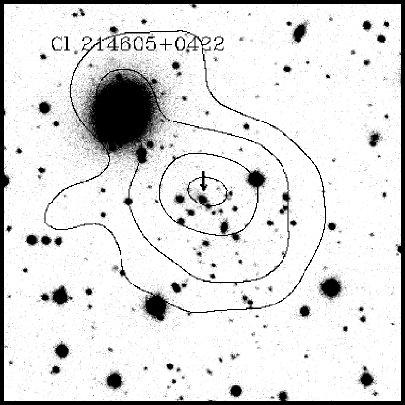
Figure 1: A 35 minute exposure R-band image of the cluster Cl214605+0422 (grayscale) obtained with the FLWO 48 inch telescope with $ROSAT$ PSPC X-ray contours superposed. The redshift of the brightest cluster galaxy (indicated by the arrow) was found to be $z=0.531$, using spectra obtained with the MMT. This object is one of the distant clusters detected in the 160 square degree survey. The image is 4.4 arcmin on a side. North is at the top; east is to the left.

4 The Cluster Contrast Parameter

Because we were required to optically vet over 200 cluster candidates, we were initially unable to obtain deep images for all clusters. We therefore obtained optical images to a sufficient depth to determine whether the X-ray cluster candidates are indeed associated with galaxy concentrations, and to measure brightest cluster galaxy magnitudes for photometric redshift estimation (Vikhlinin et al. 1998 a, b). In most instances, our data do not completely sample cluster galaxies two magnitudes fainter than the third brightest galaxy. Therefore, we were required to correct our galaxy counts to a consistent depth, as discussed in §6.1. However, first we will demonstrate that galaxy concentrations are indeed present at the locations of the extended X-ray sources using the contrast parameter introduced by Couch et al. (1991).

The contrast parameter $\sigma_{\rm cl}=N_{\rm cl}/\sigma_{\rm bg}$ (Couch et al. 1991), is a measure of the observed over-density of bright cluster galaxies against the background. Here, $N_{\rm cl}$ is the net number of galaxies within an aperture centered on the cluster, after subtracting the average background surface density measured in 20–30 randomly placed apertures surrounding the cluster. The parameter $\sigma_{\rm bg}$ is the standard deviation about the mean background value for the surrounding apertures. The contrast parameter provides a crude measure of cluster richness that is relatively insensitive to the imaging depth, but depends strongly on redshift, central galaxy concentration, and detection aperture size.

Figure 2: Histogram of the contrast parameter $\sigma_{\rm cl}$ as a function of aperture size. $\sigma_{\rm cl}$ decreases with increasing aperture size in a manner that is consistent with an isothermal galaxy surface density profile (broken line).

We demonstrate the effects of increasing aperture size and increasing imaging depth on $\sigma_{\rm cl}$ in Figures 2 & 3. In Figure 2 we examine the effect of aperture size on the contrast parameter by plotting histograms of $\sigma_{\rm cl}$ against aperture size for our sample. $\sigma_{\rm cl}$ reaches a maximum with the 0.25–0.5 Mpc apertures and declines with increasing aperture size. Within these apertures, the modal contrast is $\simeq 2.5\pm 1$. The contrast for an isothermal distribution of galaxies should decline with aperture radius roughly as $\sigma_{\rm cl}(r)\sim\ln r/r$ (shown as the broken line in Figure 2), while $\sigma_{\rm cl}(r)\sim{\rm constant}$ for a $\rho_{\rm g}\sim r^{-1}$ profile. The contrast parameter appears to decline with increasing aperture size in a manner that is roughly consistent with an isothermal profile.

In Figure 3 we plot the contrast parameter within a 1 Mpc radius as a function of imaging depth. The imaging depth, $\Delta m$, is the limiting magnitude depth relative to the brightest cluster galaxy’s magnitude. The data are for two richness class 1–2 clusters in our sample with deep imaging obtained with the ESO 3.6 m telescope. No strong dependence is found between contrast significance and imaging depth for either cluster.

Figures 2 & 3 demonstrate that the optical contrast of clusters against the background is relatively constant with imaging depth, but declines rapidly with aperture size. Both properties are due to the rapidly increasing background galaxy counts. We find that a 1 Mpc aperture strikes a good compromise between the competing demands of good cluster counting statistics and minimizing the background noise. In general, the background counts are factors of 2–3 larger than the cluster counts within a 1 Mpc aperture.

Figures 2 & 3 also show that relatively shallow imaging is effective at detecting galaxy concentrations at redshift $z\sim 0.5$. However, as is seen in Table 1 and discussed below, the contrast parameter is not a reliable measure of cluster richness. For instance, Couch et al. found that, within a 1.5 Mpc diameter aperture using a passband similar to ours, $\sigma_{\rm cl}\sim 3$ corresponds approximately to a richness class 1 cluster, and $\sigma_{\rm cl}\sim 4-6$ corresponds to a richness class 2 to 3 cluster at redshifts $z=0.5-0.7$. We do not find such a large increase in contrast with richness for our clusters (cf. Table 1). On average, our clusters show a lower contrast than Couch’s, and fall in the regime where their catalog becomes seriously incomplete. In fact, a cluster such as Cl 2146+0422, shown in Figure 1, would probably have been omitted from the Couch et al. (1991) catalog.

Figure 3: Contrast parameter, $\sigma_{\rm cl}$, plotted against imaging depth, $\Delta m$, for two deeply-imaged clusters. $\sigma_{\rm cl}$ shows no significant increase with imaging depth.

5 Comparison of Galaxy Counts Between our Distant X-ray Clusters and Nearby Abell Clusters

Here we compare the galaxy counts from our sample to those in nearby clusters by comparing the net number of galaxies within a 1 Mpc radius as a function of imaging depth. This approach has two significant advantages over direct richness estimates. First, galaxy counts within a 1 Mpc radius are more accurate than counts within a 3 Mpc radius, because the background corrections are smaller. Second, we avoid entirely the uncertain depth and aperture corrections required to estimate Abell richnesses. The primary disadvantage is that galaxy counts as a function of cluster radius and magnitude depth are generally unavailable for clusters. We remedied this situation by measuring galaxy counts toward 14 nearby Abell clusters from Digital Sky Survey (DSS) images. The clusters, with redshifts between $z=0.04-0.1$, were selected from the ROSAT Brightest Cluster Sample (BCS, Ebeling et al. 1998). Their X-ray luminosities, $L_{\rm x}(0.1-2.4)=1-6\times 10^{44}~{}{{\rm ergs\ s}^{-1}}$, roughly match the range for our distant sample, after correcting for the bandpass offset. The galaxies on the DSS images were selected and counted automatically, after correcting for photographic nonlinearity, in a nearly identical manner to our distant cluster method. For example, the galaxy selection algorithm and background field corrections were applied in a similar fashion. The expression used to compute the galaxy and background fluxes that relates intensity, $I$, to photographic density, $D$, is: $\ln I=f_{1}\times D+f_{2}\times\log(e^{BD^{C_{1}}}-1)+f_{3}\times e^{BD^{C_{2}}}+f_{4}$. The photographic nonlinearity was removed through the coefficients $f$, $B$, and $C$, which were derived by comparing the digitized photographic magnitudes of stars and galaxies from the DSS to calibrated CCD images of the same fields.

We avoided the potential errors associated with selecting the third brightest galaxy (cf. §3) by measuring depth with respect to the magnitude of the BCG. The largest uncertainty associated with this approach would be differential luminosity evolution of the BCG with respect to the remaining cluster galaxies. However, we don’t believe this to be a serious problem. The BCGs in our sample are very good standard candles to $z=0.5-0.7$ (Vikhlinin et al. 1999). The variation about their mean $R$-band luminosity is $\sigma\approx 0.3$ magnitudes. While a variation at this level would affect individual clusters, it would not significantly affect the comparison, as both samples were treated in a similar fashion. Nevertheless, this approach provides a good check on our application of the Abell richness criteria. The details of the automated DSS galaxy counts for the nearby clusters will be presented in a future paper (Whitman, McNamara, & Vikhlinin, in prep). It is worth noting in advance, however, that our automated counts agree with the ACO catalog to within the counting statistics for all clusters within this luminosity and richness range. This check provides a measure of reassurance that our comparison in Figure 4 for the 1 Mpc apertures is reliable.

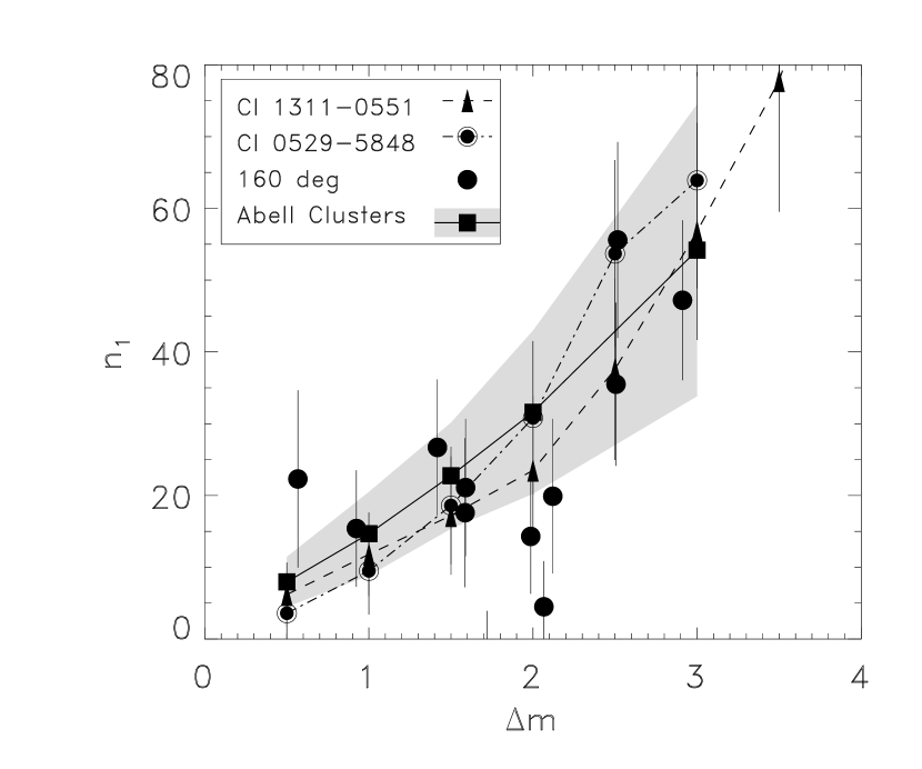
Figure 4: Plot of galaxy counts within a 1 Mpc radius aperture, $n_{1}$, vs the limiting imaging depth with respect to the BCG, $\Delta m$. The shaded region shows the $1\sigma$ plane occupied by nearby, X-ray-selected Abell clusters. The mean is indicated by connected, filled rectangles. The 160 square degree clusters are shown as indicated in the legend.

The galaxy count comparison between the BCS and 160 square degree survey clusters as a function of imaging depth is shown in Figure 4. The average number of galaxies as a function of depth within a 1 Mpc radius for the 14 nearby BCS Abell clusters is shown as connected, filled rectangles. The one $\sigma$ deviation about the mean is enclosed by the shaded region. The galaxy counts from the deep imaging of Cl 1311-0551 and Cl 0529-5848 are shown as connected points. The remaining 160 square degree clusters are shown as solid points. The error bars are one sigma Poisson estimates using the net cluster and background counts in each aperture, calculated as $\sigma=\sqrt{N_{\rm cl}+N_{\rm bg}}$.

Figure 4 shows that nearly all of the 160 square degree clusters lie within $2\sigma$ of the BCS clusters. Although a few outliers are good candidate galaxy-poor clusters, the overall agreement is quite good. We can conclude that the 160 degree survey clusters are similarly rich to the nearby BCS clusters with the same range of X-ray luminosity. In the next section, we estimate the richnesses of the distant clusters according to the Abell criteria by applying depth and aperture corrections to the galaxy counts.

6 Estimating Cluster Richnesses

6.1 Imaging Depth Corrections

Our images often do not reach a sufficient depth to sample completely to $m_{3}+2$. Therefore, we measure an incompleteness parameter for each cluster by taking the difference between the location of the peak of the instrumental magnitude histogram for all galaxies in each field and $m_{3}+2$. The incompleteness parameter, $\delta m$, is listed in Table 1. We corrected the galaxy counts assuming a cumulative luminosity function of the form $\log N(\leq m)=K+S\times m$, where $S$ is the slope of the cumulative luminosity function (Sarazin 1986). The function was normalized by the detected number of cluster galaxies, $N_{\rm g}$, as $\log N_{\rm g}^{\prime}=\log N_{\rm g}+S\delta m.$ The cluster galaxy luminosity function is poorly known for distant clusters. We therefore estimated $S$ for the sample using deep $R$-band images of Cl 1311-0551 and Cl 0529-5848, which we obtained with the European Southern Observatory’s 3.6m telescope. The cumulative distributions of galaxies, after background subtraction, are shown for each cluster in Figure 5. The curves shown are normalized to the magnitude of the brightest cluster galaxy in each cluster. Our data sample completely three magnitudes below the brightest galaxy for Cl1311-0551 and four magnitudes below the brightest galaxy for Cl1311-0551. As the modal difference between the brightest and third brightest galaxies for our 14 cluster sample is $m_{1}-m_{3}\approx 0.4$ magnitudes (the ACO value is $\approx 0.35$ magnitudes), these two clusters, if representative of our sample as a whole, reach a depth well below $m_{3}+2$. The slope of the linear fit to the data is $S=0.39\pm 0.1$. We assume from now on that the luminosity functions of the remaining clusters have this slope, and we use $S$ to correct their galaxy counts for imaging depth incompleteness as described above.

Figure 5: Plot of the logarithm of galaxy counts within a 1 Mpc radius aperture, $n_{1}$, vs the limiting imaging depth with respect to the BCG, $\Delta m$, for two, deeply-imaged clusters. The straight line fit to the data was used to apply the depth corrections to the remaining 160 degree survey objects.

6.2 Comparison Between Nearby and Distant X-ray-Selected Cluster Richnesses

After correcting our counts for imaging depth incompleteness, we computed cluster richnesses, $\Lambda_{\rm c}$, by extrapolating counts in each aperture to the 3 Mpc Abell radius. The extrapolations assume both $r^{-2}$ and $r^{-1.4}$ surface density profiles, normalized by the corrected counts within each aperture. Extrapolation, rather than direct measurement, is required because the galaxy background increases more rapidly with increasing aperture than the cluster counts. When the size of the Poisson variations in the background counts approaches the cluster signal, the cluster counts become unreliable. Although the backgrounds in the 0.25 and 0.5 Mpc apertures are only $\sim 50\%$ of the cluster counts, only a few cluster galaxies are generally present there. Therefore, the Poisson errors in the cluster counts are relatively large. On the other hand, as the aperture grows to 1 Mpc, the background becomes factors of $\sim 2-3$ larger than the cluster counts. Nonetheless, the one to three dozen net cluster galaxies present can be counted with greater precision.

Whether or not a universal galaxy surface density profile for distant clusters exists is unknown. The density profile of galaxies for a sample of 14 intermediate redshift ($z\sim 0.4$), X-ray-selected clusters was found by Carlberg et al. (1997) to follow a Navarro, Frenk, & White (1997) profile. This profile implies a steep $r^{-3}$ decline in galaxy surface density at very large radii, but a somewhat shallower decline over much of the 3 Mpc region of interest. On the other hand, the $z\mathrel{>\kern-10.00002pt\lower 3.87495pt\hbox{$\sim$}}0.5$ clusters selected optically in the Palomar Distant Cluster Survey appear to have considerably shallower, $r^{-1.4}$ profiles within the radial range considered in this sample.

We therefore analyzed our sample by applying both $r^{-1.4}$ and isothermal, $r^{-2}$ surface density profiles to our aperture corrections. In the upper panel of Figure 6, we present richnesses for 13 clusters with $\delta m<1.5$. In the lower panel, we plot richnesses for a subset of 9 clusters with smaller depth corrections, $\delta m<0.7$. The solid distribution of clusters has been corrected assuming the $r^{-2}$ profile, and the dashed distribution has been corrected for the $r^{-1.4}$ profile. The shallower, $r^{-1.4}$ profile correction gives somewhat higher richnesses compared to the $r^{-2}$ profile, as would be expected. However, the distributions do not differ greatly. Therefore, for simplicity, we adopt the $r^{-2}$ profile when deriving richnesses and richness classes (e.g., Figure 7 and Table 1), although our conclusions do not depend significantly on this assumption.

The cluster richnesses and richness classes were determined by applying the depth and aperture corrections to the $0.25,~{}0.5$, and 1 Mpc aperture counts prior to averaging them. Cluster richnesses are binned into richness classes ($RC$) mapped following the ACO catalog: $\Lambda_{\rm c}=~{}10-30,~{}31-49,~{}50-79,~{}80-129,~{}130-200,~{}200-300$ $\rightarrow RC=-1,~{}0,~{}1,~{}2,~{}3,~{}4$, respectively. The errors in the richnesses are dominated by systematics, so we adopted the extreme values from the three apertures as an error estimate (shown in Figure 7 and discussed below). Figure 6 shows that our clusters are primarily richness class 0–2. While three clusters may lie in richness classes $3-4$, their richness estimates depend on large and uncertain depth corrections (see Table 1). Their richness estimates are therefore suspect.

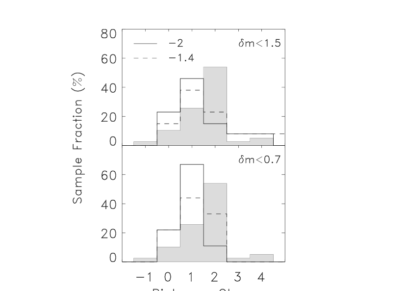
Figure 6: A comparison between the distribution of richness classes for our distant sample and the nearby X-ray sample of Edge et al. (1990) [shaded region]. The solid histogram shows the distribution of clusters corrected by an $r^{-2}$ surface density profile, while the broken distribution has been corrected using a $r^{-1.4}$ profile. The differences between the distant and nearby samples are statistically marginal.

We compare our distant cluster richnesses to the nearby $z<0.18$, X-ray-flux-limited sample of Edge et al. (1990), shown as the filled histogram in Figure 6. The richness classes and counts for most clusters in the Edge et al. sample were taken from the ACO catalog. Others were taken from Bahcall (1980) and Owen et al. (1997). Only clusters with X-ray luminosities exceeding our lower limit of $L_{\rm X}(0.5-2)\sim 0.5\times 10^{44}~{}{{\rm ergs\ s}^{-1}}$ are included. Edge’s X-ray luminosities were adjusted downward by typically a factor of two to match the $ROSAT$ band. Richnesses for five Edge et al. clusters (3C129, 0745–191, A3158, Ophiucus, Triangulum Australis) are unavailable in the literature and were thus excluded.

Overall, the richness distributions for the 160 degree survey clusters are similar to the nearby cluster distribution, if not somewhat poorer (the modal richness of the Edge et al. clusters is $RC\sim 2$, while for the 160 degree survey clusters it is $RC=1$). This difference turns, however, on only a few clusters. Our sample is simply too small to reliably discriminate between these distributions. We conclude, as we did with Figure 4, that to within the sampling precision, the nearby and distant clusters have similar richness distributions.

6.3 The X-ray Luminosity–Richness Relation

In Figure 7, we plot the 14 clusters in our sample on the $L_{\rm x}$–richness plane. For comparison, we plotted the mean $L_{\rm x}$–richness relation for $<z>=0.17$ clusters from the $ROSAT$ All Sky Survey (Briel & Henry 1993). Our clusters are plotted as solid points, while the Briel-Henry relation is the solid line. In addition, we plotted optically-selected, $z>0.5$ clusters from the Palomar Distant Cluster Survey (PDCS; Postman et al. 1996, Holden et al. 1997) as open points. The optical cluster X-ray data from Holden et al. 1997 and the Briel & Henry relation have been adjusted slightly to register the X-ray passbands. The horizontal broken line at $L_{\rm x}=0.5\times 10^{44}~{}{{\rm ergs\ s}^{-1}}$ shows the approximate luminosity of a $z=0.5$ cluster corresponding to our X-ray flux detection threshold of $f_{\rm x}\sim 2\times 10^{-14}~{}{{\rm ergs\ s}^{-1}}~{}{\rm cm}^{-2}$.

Figure 7 shows the larger fraction of our clusters lying above the Briel & Henry mean relation in such a way as to appear poorer than average, as was found in Figure 6. Nevertheless, our clusters lie well within the large scatter of the Briel & Henry relation. Given the combination of the small sample size, the large uncertainties in the richness corrections, and the ample spread in the Briel–Henry relation, we can only conclude that our clusters may be a bit poorer than average, but they are within the expected range for nearby clusters with similar X-ray luminosities.

Figure 7: The $L_{\rm x}$–Richness relation for our sample (solid points), $z\mathrel{>\kern-10.00002pt\lower 3.87495pt\hbox{$\sim$}}0.5$ PDCS clusters (open points), and the local relation from Briel & Henry (1993) [solid line]. The dashed-dotted line shows the flux limit of our survey. The richness estimates for the three richness class 3 and 4 clusters depend on large richness corrections. Therefore, they may have been systematically overestimated.

On the other hand, the optically-selected, PDCS clusters have a similar richness distribution to our X-ray clusters, yet few, if any, are detected in X-rays. Only 3 of 16 similarly distant PDCS clusters were detected in X-rays, and even these may be background sources (Holden et al. 1997). A similar trend was noted by Bower et al. (1994) using clusters selected from the Couch et al. (1991) catalog. The distributions of our clusters and the PDCS clusters shown in Figure 7 are clearly segregated by X-ray luminosity. Therefore, based on the analysis of these small samples, our survey and the PDCS are apparently not detecting similar mass concentrations.

The reason why this would be so is not entirely clear. However, a serious and well-known problem associated with optically-detected clusters would be the tendency to misidentify superposed but physically-distinct groups of galaxies along a sight line as a physical cluster (see Postman et al. 1996, Oke, Postman, & Lubin 1998). Furthermore, optical catalogs may be prone to contain real, galaxy-rich mass concentrations which have not yet virialized (Peebles 1993), yet they can be confused with rich, virialized clusters. On the other hand, optical selection techniques would be sensitive to optically rich but X-ray-faint galaxy clusters that would otherwise be missed by X-ray surveys. This last hypothesis, intriguing as it may be, is difficult to understand, as significant X-ray emission is expected from clusters in most cosmological scenarios (Bower et al 1997).

In a recent study of the Couch et al. (1991) catalog of clusters, Bower et al. (1997) found concordant galaxy velocities for most clusters. Based on an analysis of the radial velocity histograms, they argued that the Couch objects were real mass concentrations. However, their velocity dispersions were nearly a factor of two larger than nearby clusters with comparable X-ray luminosities. Conversely, their X-ray luminosities were an order of magnitude smaller than nearby clusters with similar velocity dispersions. Bower et al. (1997) concluded that the Couch cluster velocity dispersions do not reflect the clusters’ virial temperature. Rather, the velocity dispersions are either inflated by infalling galaxies on nearly radial orbits, or the clusters are embedded in large-scale filaments oriented along the line of sight. Since the infall scenario seems to imply an unrealistically rapid rate of infall, the latter scenario seems more likely to be true. The essential point is that optical clusters may poorly represent the general population of distant clusters (cf. Donahue et al. 2001). The comparison between our clusters and the PDCS clusters, shown in Figure 7, supports this interpretation. Most importantly, the new results in this paper demonstrate that X-ray emission is a reliable tracer of cluster-scale mass concentrations in the distant Universe.

7 Conclusions

We have estimated richnesses for some of the most distant clusters from the 160 square degree cluster survey (Vikhlinin et al. 1998a, b) using three methods. We found that our survey is efficient at detecting rich galaxy contrations at redshifts beyond $z=0.5$. These clusters have X-ray luminosities between $L_{\rm x}(0.5-2)\sim 0.5-2.6\times 10^{44}~{}{{\rm ergs\ s}^{-1}}$, and Abell richness classes typically between $0-2$. The richness distribution of the distant, 160 square degree clusters is similar to the distribution of nearby clusters with similar X-ray luminosities. Clusters have evidently evolved by less than $0.5-1$ richness classes between redshifts of $1/2$ and today. We find marginal evidence that our distant clusters are somewhat poorer than the average nearby cluster, although deep, multicolor imaging would be required to confirm this.

We compared our sample richnesses to those for a sample of equally distant, optically-selected clusters from the Palomar Distant Cluster Survey that have been observed by $ROSAT$ (Holden et al. 1997). Although the PDCS clusters are comparably rich, they have significantly lower X-ray luminosities compared to our clusters. This segregation in $L_{\rm x}-$richness plane is not understood, but may reflect the tendency for optical surveys to detect superpositions of galaxies, and unvirialized mass concentrations associated with large-scale filaments.

Table 1: Distant X-ray Clusters

Cluster	$z$	$f_{\rm x}(0.5-2)$	$L_{\rm x}(0.5-2)$	$\delta m$	$\Delta m$	$\sigma_{\rm cl}$	$n_{1}$	RC
		$10^{-14}~{}{\rm cgs}$	$10^{44}~{}{\rm erg~{}s}^{-1}$	mag	mag
0030$+$2618	0.500	24.3	2.6	0.43	2.12	2.1	$20\pm 11$	1
0521$-$2530	0.581	17.6	2.6	0.79	1.72	…	$-5\pm 9$	0
0522$-$3625	0.472	18.4	2.3	0.03	2.51	2.0	$56\pm 13$	1
0529$-$5848	0.466	5.6	0.6	0.00	3.0	1.6	$64\pm 15$	1
0847$+$3449	0.560	12.2	1.7	0.55	1.59	1.4	$18\pm 10$	0
0848$+$4456	0.574	3.3	0.5	1.73	0.57	2.8	$22\pm 12$	4
0858$+$1357	0.500	6.4	0.8	0.99	1.59	2.1	$21\pm 9$	4
0951$-$0128	0.567	7.1	1.0	0.58	1.99	2.9	$14\pm 8$	1
0956$+$4107	0.600	15.6	2.4	1.44	0.92	1.2	$15\pm 8$	3
1002$-$0808	0.520	8.6	1.1	0.96	1.42	2.3	$27\pm 9$	2
1311$-$0551	0.461	13.7	1.3	0.00	3.0	2.2	$57\pm 15$	2
1354$-$0221	0.546	14.5	2.0	0.00	2.91	3.0	$47\pm 11$	1
2146$+$0422	0.531	13.8	1.7	0.21	2.07	1.0	$5\pm 6$	0
2328$+$1453	0.497	7.6	0.9	0.08	2.51	2.2	$35\pm 11$	1

References

- (1)
- (2) Abell, G.O. 1958, ApJS, 3, 211
- (3)
- (4) Abell, G.O., Corwin, H.G., Jr., Olowin, R.P. 1989, ApJS, 70, 1 (ACO)
- (5)
- (6) Bahcall, N. 1980, ApJ, 238, L117
- (7)
- (8) Bahcall, N.A., Fan, X, Cen, R. 1997, ApJ, 485, L53
- (9)
- (10) Bower, R.G., Böhringer, H., Briel, U.G., Ellis, R.S., Castander, F.J., Couch, W.J. 1994, MNRAS, 268, 345
- (11)
- (12) Bower, R.G., Castander, F.J., Couch, W.J., Ellis, R.S., Böhringer, H. 1997, MNRAS, 291, 353
- (13)
- (14) Briel, U.G. Henry, J.P. 1993, AA, 278, 379
- (15)
- (16) Burg, R., Giacconi, R., Forman, W., Jones, C. 1994, ApJ, 422, 37
- (17)
- (18) Carlberg, R.G. Yee, H.K.C., Ellingson, E., Morris, S.L., Abraham, R., Gravel, P., Pritchett, C.J., Smecker-Hane, T., Hartwick, F.D.A., Hesser, J.B., Hutchings, J.B., & Oke, J.B., 1997, ApJ, 485, L13
- (19)
- (20) Collins, C.A., Burke, D.J., Romer, A.K., Sharples, R.M., Nichol, R.C. 1997, ApJ, 479, L117
- (21)
- (22) Couch, W.J., Ellis, R.S., Malin, D.F., MacLaren, I. 1991, MNRAS,249, 606
- (23)
- (24) David, L.P., Arnaud, K.A., Forman, W., Jones, C. 1990, ApJ, 356, 32
- (25)
- (26) Donahue, M., Mack, J., Lee, P., Postman, M., Dickinson, M., Voit, G.M. 2001, ApJ, submitted
- (27)
- (28) Dressler, A., Oemler, A., Jr., Couch, W.J., Smail, I., Ellis, R.S., Barger, A., Butcher, H., Poggianti, B.M., Sharples, R.M., 1997, ApJ, 490, 577
- (29)
- (30) Ebeling, H., Edge, A.C., Böhringer, H., Allen, S.W., Crawford, C.S., Fabian, A.C., Voges, W., & Huchra, J.P. 1998, MNRAS, 301, 881
- (31)
- (32) Edge, A.C., Stewart, G.C., Fabian, A.C., Arnaud, K.A., 1990, MNRAS, 245, 559
- (33)
- (34) Eke, V.R.. Cole, S., and Frenk, C.S. 1996, MNRAS, 282, 263
- (35)
- (36) Evrard, A.E., Metzler, C.A., Navarro, J.F. 1996, ApJ, 469, 494
- (37)
- (38) Frenk, C.S., Evrard, A.E., White, S.D.M., Summers, F.J. 1996, ApJ, 472, 460
- (39)
- (40) Gioia, I.M. 1997, astro-ph/9712003
- (41)
- (42) Gioia, I.M., Henry, J.P., Mullis, C.R., Voges, W., Briel, U.G., Böehringer, H. & Huchra, J.P., 2001, ApJ Letters, in press (astro-ph/0102332)
- (43)
- (44) Henry, J.P., Gioia, I.M., Maccacaro, T., Morris, S.L., Stocke, J.T., Wolter, A. 1992, ApJ, 386, 408
- (45)
- (46) Henry, J.P., Gioia, I.M., Mullis, C.R., Voges, W., Briel, U.G., Böehringer, H. & Huchra, J.P., 2001, ApJ Letters, in press
- (47)
- (48) Holden, B.P., Romer, A.K., Nichol, R.C., Ulmer, M.P. 1997, AJ, 115, 1701
- (49)
- (50) Jones, L.R., Scharf, C., Ebeling, H. Perlman, E., Wegner, G., Malkan, M., Horner, D. 1998, ApJ, 495, 100
- (51)
- (52) Kaiser, N. 1986, MNRAS, 222, 323
- (53)
- (54) Lubin, L. & Postman, M. 1996, AJ, 111, 1795
- (55)
- (56) Luppino, G.A., Gioia, I.M. 1995, ApJ, 445, L77
- (57)
- (58) Markevitch, M. 1998, astro-ph/9802059
- (59)
- (60) Mathiesen, B. & Evrard, A.E. 1998, MNRAS, 295, 769
- (61)
- (62) Mushotzky, R.F., Scharf, C.A. 1997, ApJ, 482, L13
- (63)
- (64) Navarro, J.F., Frenk, C.S., & White, S.D.M. 1996, ApJ, 462, 563
- (65)
- (66) Oke, J.B., Postman, M., Lubin, L.M. 1998, AJ, 116, 549
- (67)
- (68) Owen, F.N., Ledlow, M.J., Morrison, G.E., Hill, J.M. 1997, ApJ, 488, L15
- (69)
- (70) Peebles, P.J.E. 1993, “Principles of Physical Cosmology,” Princeton University Press, p. 634
- (71)
- (72) Postman, M., Lubin, L., Gunn, J.E., Oke, J.B., Hoessel, J.G., Schneider, D.P., Christensen, J.A. 1996, AJ, 111, 615
- (73)
- (74) Rosati, P., Della Ceca, R., Norman, C., Giacconi, R. 1998, ApJ, 492, L21
- (75)
- (76) Richstone, D., Loeb, A., Turner, E.L. 1992, ApJ, 393, 477
- (77)
- (78) Sarazin, C.L. 1980, ApJ, 236, 75
- (79)
- (80) Sarazin, C.L. 1986, Rev. Mod. Phys. 58, 1
- (81)
- (82) Tucker, W.H., Tananbaum, H., Remillard, R.A. 1995, ApJ, 444, 532
- (83)
- (84) Viana, P.T.P & Liddle, A.R. 1998, astro-ph/9803244
- (85)
- (86) Vikhlinin, A. McNamara, B.R., Forman, W., Jones, C., Hornstrup, A., Quintana, H. 1998a, ApJ, 502, 558
- (87)
- (88) Vikhlinin, A. McNamara, B.R., Forman, W., Jones, C., Hornstrup, A., Quintana, H. 1998b, ApJ, 498, L21
- (89)
- (90) White, S.D.M., Rees, M.J. 1978, MNRAS, 183, 341
- (91)
- (92) Yee, H.K.C. & Lopez-Cruz, O. 1999, ApJ, 117, 1985
- (93)