Another Channel to detect Close-in Binary
Companions via Gravitational Microlensing

Abstract

Gaudi & Gould (1997) showed that close companions of remote binary systems can be efficiently detected by using gravitational microlensing via the deviations in the lensing light curves induced by the existence of the lens companions. In this paper, we introduce another channel to detect faint close-in binary companions by using microlensing. This method utilizes a caustic-crossing binary lens event with a source also composed of binary stars, where the companion is a faint star. Detection of the companion is possible because the flux of the companion can be highly amplified when it crosses the lens caustic. The detection is facilitated since the companion is more amplified than the primary because it, in general, has a smaller size than the primary, and thus experiences less finite source effect. The method is extension of the previous one suggested to detect close-in giant planets by Graff & Gaudi (2000) and Lewis & Ibata (2000) and further developed by Ashton & Lewis (2001). From the simulations of realistic Galactic bulge events, we find that companions of K-type main sequence or brighter can be efficiently detected from the current type microlensing followup observations by using the proposed method. We also find that compared to the method of detecting lens companions for which the efficiency drops significantly for binaries with separations $\mathrel{\hbox{\hbox to0.0pt{\hbox{\lower 4.0pt\hbox{$\sim$}}\hss}\hbox{$<$}}}0.2$ of the angular Einstein ring radius, $\theta_{\rm E}$, the proposed method has an important advantage of being able to detect companions with substantially smaller separations down to $\sim({\cal O})10^{-2}\theta_{\rm E}$.

1 Introduction

Observationally constraining the characteristics of faint close-in binary companions is important to understand the process of star formation and evolution. For example, mass transfer between the binary components through Roche lobe overflow could alter the physical processes of stellar evolution (Iben & Tutukov 1984; Han, Tout, & Eggleton 2000). Theoretical investigations about the origin of Type Ia supernova are also based on the observations of close binaries (Nomoto & Sugimoto 1977; Li & van den Heuvel 1997; Langer et al. 2000). Another possible outcome of close binary evolution is a merger during the late stage of a common envelope phase (Iben & Livio 1993; Armitage & Livio 2000; Taam & Sandquist 2000), whose physical parameters should be constrained by observations.

Detection of faint close-in binary companions is also important for the accurate determination of the stellar mass function. The mass function of stars is derived from their luminosity function by using the mass-luminosity relation. In this determination, however, if the mass function is derived without considering unresolved faint binary companions, the resulting stellar mass function will be biased towards larger masses. Even if they are taken into consideration, the constructed mass function will suffer from large uncertainties because the uncertainties in the properties (the frequency and the mass ratio distribution) of the unresolved binaries will directly propagate into the resulting mass function (Kroupa, Tout, & Gilmore 1991; Reid 1991; Reid & Gizis 1997).

Faint close-in binary companions can be detected by using various methods, e.g. direct imaging by using high-resolution interferometers, astrometric measurements of the primary motion, spectroscopic radial velocity measurements, and photometric measurements of the light variation caused by occultation (eclipsing). However, these methods have limitations in detecting and characterizing various types of binaries. For example, the direct imaging and astrometric methods have limited applicabilities only to nearby stars. The spectroscopic method can be applied to detect binaries located at large distances. However, determining the mass ratio between the binary components by using this method requires that both components should be bright for the construction of the individual stars’ radial velocity curves, limiting the applicability of the method. Constraining the physical properties of eclipsing binary companions suffers from similar limitation. Therefore, invention of complementary methods to detect and characterize various types of binaries is important.

Close binaries can also be detected and characterized by using microlensing. Detecting binary companions via microlensing is possible because if events are caused by lenses composed of binaries, the resulting light curves can exhibit noticeable deviations from the smooth and symmetric ones of single lens events. In addition, one can constrain the physical properties of the binaries (the mass ratios and the scaled projected separation between the binary components) by fitting model light curves to the observed one.

In this paper, we introduce another method of detecting and characterizing faint close-in binary companions by using microlensing. This method utilizes caustic-crossing binary lens events with a source also composed of binary stars, where the companion is a faint star. Detecting the source companion is possible because the flux from the companion can be highly amplified when it crosses the lens caustics. This method is extension of the previous one suggested to detect close-in giant planets by Graff & Gaudi (2000) and Lewis & Ibata (2000) and further developed by Ashton & Lewis (2001).

The paper is organized in the following way. We describe the basics of microlensing in § 2. We perform simulations of example Galactic bulge events in § 3 and evaluate the detectability of the deviations induced by binary source companions for the example events in § 4. A brief summary of the results and discussion about the advantages and disadvantages of the proposed method compared to that of detecting lens companions are included in § 5.

2 Basics of Microlensing

The light curve of a single point-source event caused by a single point-mass lens is represented by a simple analytic form of

$$A_{0}={u^{2}+2\over u\sqrt{u^{2}+4}},$$ (1)

where $u$ is the lens-source separation normalized by the angular Einstein ring radius. The Einstein ring radius is related to the physical parameters of the lens by

$$\theta_{\rm E}=\sqrt{4GM\over c^{2}}\left({1\over D_{\rm ol}}-{1\over D_{\rm os}}\right)^{1/2},$$ (2)

where $M$ is the mass of the lens and $D_{\rm ol}$ and $D_{\rm os}$ represent the distances from the observer to the lens and source, respectively.

The light curve of a caustic-crossing binary lens event with a source composed of also binaries, which is the target event for followup monitoring to detect faint binary source companions by using the proposed method, deviates from the standard form in eq. (1) due to various effects. These include the effects of lens and source binarity, and the finite source effect. In the following subsections, we describe the basics of these effects.

2.1 Binary Lens Events

If an event is caused by a binary lens system, the locations of the individual images are obtained by solving the lens equation expressed in complex notations by

$$\zeta=z+\frac{m_{1}}{\bar{z}_{1}-\bar{z}}+\frac{m_{2}}{\bar{z}_{2}-\bar{z}},$$ (3)

where $m_{1}$ and $m_{2}$ are the mass fractions of the individual lenses, $z_{1}$ and $z_{2}$ are the positions of the lenses, $\zeta=\xi+i\eta$ and $z=x+iy$ are the positions of the source and images, and $\bar{z}$ denotes the complex conjugate of $z$ (Witt 1990). Note that all these lengths are dimensionless because they are normalized by the combined Einstein ring radius, which is equivalent to the Einstein ring radius of a single lens with a mass equal to the total mass of the binary. Depending on the source position with respect to the lenses, there exist 3 or 5 solutions for the lens equation, and thus the same number of images. The amplification of each image $A_{i}$ is given by the Jacobian of the lens equation evaluated at the image position, i.e.,

$$A_{0,i}=\left(\frac{1}{|{\rm det}\ J|}\right)_{z=z_{i}};\ \ {\rm det}\ J=1-{\partial\zeta\over\partial\bar{z}}{\overline{\partial\zeta}\over\partial\bar{z}}.$$ (4)

Then, the total amplification is obtained by summing the amplifications of the individual images, i.e. $A_{0}=\sum A_{0,i}$.

The fundamental difference in the geometry of a binary lens system from that of a single point-mass lens is the formation of caustics. The caustic refers to the source position on which the amplification of a point source event becomes infinity, i.e., det $J=0$. The set of caustics forms closed curves. The caustics takes various sizes and shapes depending on the projected separation $b$ (normalized by $\theta_{\rm E}$) and the mass ratio $q$ between the lens components. The probability of caustic crossing is maximized when the binary separation is equivalent to $\theta_{\rm E}$. Whenever a source crosses the caustics, an extra pair of images appears (or disappears). Hence the light curve of a caustic-crossing binary lens event is characterized by sharp spikes. Since the caustics form a closed curve, the source of a caustic-crossing event crosses the caustic at least twice. Although the first caustic crossing is unlikely to be resolved due to its unpredictable and swift passage, it can be inferred from the enhanced amplification. Then, by preparing intensive followup observations, resolving the second caustic crossing is possible. From the surveys (EROS: Aubourg et al. 1993; MACHO: Alcock et al. 1993; OGLE: Udalski et al. 1993; DUO: Alard & Guibert 1997) and followup observations (MPS: Rhie et al. 1999; PLANET: Albrow et al. 1998; MOA: Abe et al. 1997), numerous binary lens event candidates have been detected and a significant fraction of them are caustic-crossing events (Alcock et al. 2000).

2.2 Finite Source Effect

In most parts, the light curve of an observed caustic-crossing binary lens event is well described by the point-source approximation. However, the part of the light curve near and during the caustic crossing deviates from this approximation. This is because the source star in reality is not a point source and the gradient of the amplification near the caustics is very large. As a result, different parts of the source star disk are amplified by considerably different amounts even with small differences in distance to the caustics (Schneider & Weiss 1986; Witt & Mao 1994).

The light curve of an extended source event is given by the intensity-weighted amplification averaged over the source star disk, i.e.,

$$A=\frac{\int^{2\pi}_{0}\int^{r_{\star}}_{0}I(r,\theta)A_{0}(\left|\mbox{\boldmath$r$}-\mbox{\boldmath$r$}_{L}\right|)r\ dr\ d\theta}{\int^{2\pi}_{0}\int^{r_{\star}}_{0}I(r,\theta)r\ dr\ d\theta},$$ (5)

where $r_{\star}$ is the radius of the source star, $I(r,\theta)$ is the surface intensity distribution of the source star, and the vectors $r$ and $\mbox{\boldmath$r$}_{L}$ represent the displacement vector of the center of the source star with respect to the lens and the orientation vector of a point on the source star surface with respect to the center of the source star, respectively. Consequently, the amplification does not become infinite even during the caustic crossing.

2.3 Binary Source Events

The light curve of an event with a source composed of double stars (binary source event) is very simple, as it is just the linear sum of the two light curves of the individual single source events (Griest & Hu 1992). Since the baseline flux is also the sum of the (unamplified) fluxes from the two source stars, the amplification becomes

$$A=\frac{A_{1}F_{0,1}+A_{2}F_{0,2}}{F_{0,1}+F_{0,2}},$$ (6)

where $F_{0,i}$ and $A_{i}$ are the baseline fluxes and the amplifications of the individual single source events and the subscripts $i=1$ and $2$ denote the primary and the companion source stars, respectively.

3 Simulations

The detectability of the light curve deviations induced by close-in binary source companions depends on various combinations of many parameters such as those characterizing the binary source system (e.g., the projected separation and the relative phase between the source components) and the individual component source stars (e.g., the brightness and size). Consequently, it is difficult to present the detection efficiency as a function of a couple of parameters. Therefore, we choose to evaluate the detectability by testing example light curves produced from the simulations of typical Galactic bulge events. The simulations are performed in the following ways.

Table 1: The adopted values of the physical parameters of the source stars for the tested example lensing events. The values are adopted from Allen (1973).

stellar	absolute	radius
type	magnitude	($R_{\odot}$)
Clump Giant	+2.9	4.0
G0 Dwarf	+4.4	1.04
K0 Dwarf	+5.9	0.85
M0 Dwarf	+9.0	0.63

For the source stars, we test various combinations of stellar types, which well characterize the individual source components. In Table 1, we list the source stellar types of the tested events along with the absolute magnitudes and radii, which are adopted from Allen (1973). In the simulation, we assume that each source star has a uniform surface brightness distribution over its disk and it is located at $D_{\rm os}=8$ kpc. We also assume that the motion of each source is rectilinear. This is not only because the changes of the source positions caused by their orbital motion will be small during the caustic crossings, but also because what directly affects the detectability are the instantaneous projected separation, $\ell$ (normalized by $\theta_{\rm E}$), and the phase angle, $\alpha$, between the source components at the time of caustic crossing.

For the lens system, we assume that the mass ratio and the projected separation between the lens components are $q=0.5$ and $b=1.2$. The assumed Einstein ring radius crossing timescale (Einstein timescale) of the events is $t_{\rm E}=27$ days, which corresponds to the value of a Galactic bulge event caused by a lens with a total mass and location of $\sim 0.3\ M_{\odot}$ and $D_{\rm ol}\sim 6$ kpc under the assumed lens-source transverse speed of $v\sim 150\ {\rm km}\ {\rm s}^{-1}$.

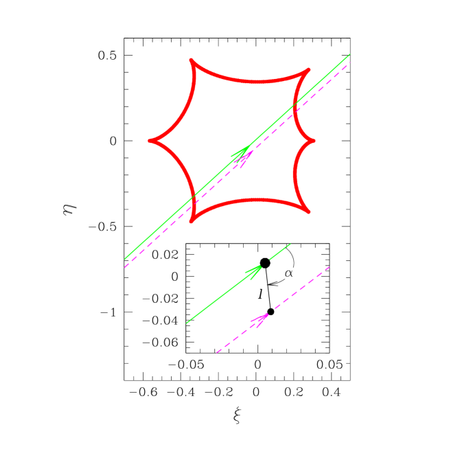
Figure 1: The location of the caustics (the closed figure drawn by a thick solid line) and the source star trajectories (straight lines) of one of the tested caustic-crossing binary lens events with double source stars. The coordinates are chosen so that the center of mass of the binary lens is at the origin. Both lenses are on the $\xi$ axis and the heavier lens is to the right. The separation and the mass ratio between the binary lens components are $b=1.2$ and $q=0.5$. The inset shows the locations of the binary source stars and the phase angle at a particular moment.

In Figure 1, we present the caustics of the lens system and the source trajectories of one of the tested example events. We note that other tested events have similar trajectories except the variations caused by the differences in the values of $\ell$ and $\alpha$.

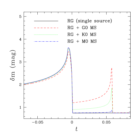
Figure 2: The light curves of a caustic-crossing binary lens event with a source also composed of binary stars where the primary is a red clump giant. The curves with different line types represent those expected when the primary source is accompanied by companions of G0, K0, and M0 main-sequence stars, respectively. The time is normalized by the Einstein time scale and it is measured from the moment when the center of the primary star crosses the caustic. The source stars have a common separation and a phase angle of $\ell=0.1$ and $\alpha=160^{\circ}$.

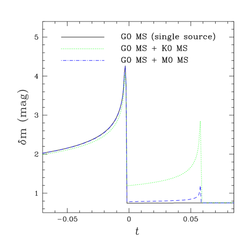
Figure 3: Similar light curves as those in Fig. 2, but for events with different combinations of source stellar types. The individual light curves are those expected when the primary of G0 main-sequence is accompanied by companions of K0 and M0 main-sequence stars, respectively. The source stars have a common separation and a phase angle of $\ell=0.1$ and $\alpha=160^{\circ}$.

In Figures 2 and 3, we present the light curves of events resulting from the various combinations of source stellar types. We present only the part of the light curve around the second caustic crossing of the primary, because high time-resolution observation is possible at around this time. For the light curves in Fig. 2, the primary source star is a red clump giant (RG) and the corresponding companions are G0, K0, and M0 main-sequence (MS) stars, respectively. For the light curves in Fig. 3, the primary is a G0 main-sequence and the companions are K0 and M0 main-sequence stars, respectively. Note that the two tested stellar types of the primary source are the typical ones of Galactic bulge events. For these events, we assume a common separation and a phase angle of $\ell=0.1$ and $\alpha=160^{\circ}$. Since the Einstein ring radius projected on the source plane of the example events is $\tilde{r}_{\rm E}=r_{\rm E}D_{\rm os}/D_{\rm ol}\sim 2.6$ AU, the assumed source separation corresponds to $\sim 0.25$ AU or $\sim 56\ R_{\odot}$. We define $\alpha$ as the angle between the primary source trajectory and the line connecting the primary and secondary source stars measured in the clockwise sense (see the inset in Fig. 1). From the figures, one finds that the part of the light curve during the caustic crossing of the secondary source is spikier than the part during the primary source caustic crossing, implying that the secondary is more highly amplified. This is because the secondary, in general, has a smaller size than the primary, and thus experiences less finite source effect.

Figure 4: Light curves of binary lens events occurred on binary source stars with various projected separations. The stellar types of the source stars are a red clump giant for the primary and a K0 main sequence for the companion. The assumed source orientation angle is $\alpha=180^{\circ}$.

To investigate the dependency of the detectability on the binary source separation, we also perform simulations of events occurred on a binary source stars with various values of $\ell$, and the resulting light curves are presented in Figure 4. For these events, the stellar types of the source stars are a red clump giant for the primary and a K0 main sequence for the companion, respectively. We test four cases of source separation of $\ell=$0.01, 0.05, 0.1, and 0.15. To see the dependency of the detectability only on the separation, we assume $\alpha=180^{\circ}$, implying that both stars are aligned and move along a common trajectory.

We also investigate the dependency of the detectability on the relative source phase by producing light curves of events occurred on source stars with various phase angles. In Figure 5, we present the resulting light curves. We test five cases of the phase angle of $\alpha=0^{\circ}$, $45^{\circ}$, $90^{\circ}$, $135^{\circ}$, and $180^{\circ}$. For these events, we also assume a red clump giant primary and a K-type main sequence companion. The source stars have a common separation of $\ell=0.1$.

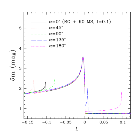
Figure 5: Light curves of binary lens events occurred on binary source stars with various phase angles. The assumed stellar types of the primary and companion are a red clump giant and a K-type main sequence, respectively. The source stars have a common separation of $\ell=0.1$.

4 Detectability Evaluation

In this section, we evaluate the detectability of the binary source induced deviations for the events produced by simulations in the previous section.

First, to be readily noticed, the light curve should deviate from that of a single source event with a significant fractional deviation. The major part of the binary source event light curve is well approximated by that of a single source event with a baseline source flux equal to the sum of the fluxes from both source stars. We, therefore, define the fractional excess amplification by

$$\epsilon={A-A_{\rm s}\over A_{\rm s}},$$ (7)

where $A$ and $A_{\rm s}$ represent the amplifications of the binary and single source events, respectively. Then, we assume that the source companion can be detected if the fractional deviation is greater than a threshold value of $\epsilon_{\rm th}$.

Table 2: The durations of deviations induced by the binary source companions for the tested example lensing events. For the definition of $t_{\rm dur}$, see § 4.

source stars			$t_{\rm dur}$	related
stellar type	separation ($\theta_{\rm E}$)	phase angle	(hrs)	figure
RG + G0 MS	0.1	$160^{\circ}$	46.0	Fig. 2
RG + K0 MS	–	–	32.4	–
RG + M0 MS	–	–	0.0	–
G0 MS + K0 MS	–	–	46.0	Fig. 3
G0 MS + M0 MS	–	–	0.0	–
RG + K0 MS	0.01	$180^{\circ}$	4.5	Fig. 4
–	0.05	–	28.5	–
–	0.1	–	28.5	–
–	0.15	–	28.5	–
RG + K0 MS	0.1	$0^{\circ}$	4.5	Fig. 5
–	–	$45^{\circ}$	7.8	–
–	–	$90^{\circ}$	5.8	–
–	–	$135^{\circ}$	5.2	–
–	–	$180^{\circ}$	28.5	–

Second, even if the fractional deviation is substantial, the deviation cannot be detected if the absolute amount of the deviation is smaller than the photometric uncertainty. Currently, microlensing followup observations are being (or planned to be) carried out by using the difference image analysis method for better photometric precision (D. Bennett, private communication). This method measures the light variation by subtracting an observed image from a convolved and normalized reference image of the same field (Tomaney & Crotts 1996; Alard & Lupton 1998). Then, the signal measured on the subtracted image is proportional to the source flux variation, i.e. $S\propto F_{0}(A-1)$, while the noise originates from both the source and background flux, i.e. $N\propto F_{0}A+B$, and thus the resulting signal-to-noise ratio is approximated by

$$S/N\sim F_{0}(A-1)\left({t_{\rm exp}\over F_{0}A+\langle B\rangle}\right)^{1/2},$$ (8)

where $F_{0}=F_{0,1}+F_{0,2}$ is the total baseline flux of the source stars, $t_{\rm exp}=2$ min is the adopted exposure time, and $\langle B\rangle$ is the average background flux within the point spread function (PSF). We assume that the observations are carried out in $I$ band by using a 1 m telescope with a CCD camera that detects $12\ e^{-}\ {\rm s}^{-1}$ for a star with $I=20$ mag. Terndrup (1988) determined that the dereddened background surface brightness contributed by bulge stars is $\mu_{I}\sim 17.6\ {\rm mag}$ ${\rm arcsec}^{-2}$. With the adopted mean extinction of $\langle A_{I}\rangle=1.5$ towards the Galactic bulge field (Stanek 1996), and additional 30% background flux from disk stars (Terndrup 1988) and sky background flux contribution of $\sim 1/4$ of stellar background, the average background flux within the PSF (with an angular area of $\Omega_{\rm psf}\sim 3.1\ {\rm arcsec}^{2}$) becomes $\langle B\rangle\sim 560\ e^{-1}\ {\rm s}^{-1}$. Once the signal-to-noise ratio is computed, the uncertainty of the light variation measurement in magnitude is computed by

$$\sigma={\delta F/F\over 0.4\ {\rm ln}\ 10}\sim{1.09\over S/N},$$ (9)

where $\delta F/F$ is the fractional uncertainty in the measured flux. Then, if the deviation occurs when $A\sim 2$, the signal-to-noise ratio becomes $S/N\sim 14$ for the event with the primary source of the clump giant, and thus the photometric uncertainty is $\sigma\sim 0.08$ mag. For the event with the primary source of the G0 main-sequence, the signal-to-noise ratio is $S/N\sim 3.7$ and the corresponding photometric uncertainty is $\sigma\sim 0.29$ mag.

The detection is additionally restricted by the duration of the deviations, $t_{\rm dur}$. We, therefore, estimate $t_{\rm dur}$ for the example events by defining $t_{\rm dur}$ as the length of time period during which the fractional and absolute deviations greater than $\epsilon_{\rm th}=0.1$ and $3\sigma$ level, respectively. The resulting values of $t_{\rm dur}$ of the individual example events are listed in Table 2. Considering the monitoring frequency of the current followup observations of $\sim 2\ {\rm hr}^{-1}$, we assume that the deviation can be detected if it continues for $t_{\rm dur}\geq 5\ {\rm hr}$.

The findings from the evaluation of the detectability are summarized as follows:

1. For both red clump giant and G-type main-sequence primaries, we find that deviations induced by source companions brighter than K-type main-sequence or brighter can be efficiently detected by using the proposed method. However, detecting deviations induced by M-type main-sequence companions will be difficult.

2. In addition, we find that with the proposed method it will be possible to detect companions with separations as small as $\ell\sim 0.01$. For a typical event with $\tilde{r}_{\rm E}\sim 2$ – 3 AU, this separation corresponds to $\sim 5\ R_{\odot}$. Considering that the size of the a clump giant is $\sim 4\ R_{\odot}$, this implies that one can detect companions of nearly contact binary systems. We also find that as long as the separation is larger than the limiting value, the dependency of the detectability on the source separation is weak.

3. Unlike the weak dependency on $\ell$, we find that the detectability depends strongly on $\alpha$: it will be easier to detect the deviation if it occurs after the primary caustic crossing. Although it will be possible to detect the deviation occurred before the primary caustic crossing, the duration of the deviation is significantly shorter than that of the deviation occurred after the primary caustic crossing. This is because the amplification of the primary source flux at the time of deviation is high, and thus the fractional deviation caused by the companion is low.

5 Summary and Discussion

In this paper, we propose a new method of detecting faint close-in stellar companions by using microlensing. The method utilizes a caustic-crossing binary lens event with a source also composed of binary stars, in which the companion is a faint star. The detection is possible because the flux from the companion can be highly amplified when it crosses the lens caustic and is facilitated because the companion is likely to be more amplified than the primary due to the smaller size of the companion. From the simulations of Galactic bulge events under realistic conditions, we find that companions with K-type main-sequence or brighter of binary lens systems with separations down to $\sim({\cal O})10^{-2}$ of the angular Einstein ring radius can be effectively detected by using the proposed method from the current type followup observations.

The proposed method of detecting source companions has both advantages and disadvantages compared to that of detecting lens companions. The most important disadvantage is that very faint or dark companions cannot be detected by using the proposed method, while the latter method can detect companions regardless of their luminosities. However, the proposed method has an important advantage of being able to detect very close companions with separations as small as $\sim({\cal O})10^{-2}\theta_{\rm E}$. By contrast, the efficiency of the latter method drops rapidly for binaries with separations $\mathrel{\hbox{\hbox to0.0pt{\hbox{\lower 4.0pt\hbox{$\sim$}}\hss}\hbox{$<$}}}0.2\theta_{\rm E}$ (Gaudi & Gould 1997). Therefore, the proposed method will make microlensing an important tool to detect binary companions by complementing the previous one. In addition, since one can obtain the color and spectral information of the companion from followup multi-band photometric and spectroscopic observations performed during the deviation by taking advantage of its highly amplified flux, one can characterize the stellar type of the companion.

We would like to thank to P. D. Sackett for making useful comments about the paper. This work was supported by the grant (20006-113-03-2) of the Korea Science & Engineering Foundation (KOSEF).

References

- [1] Abe F., et al., 1997, in Variable Stars and Astrophysical Returns of Microlensing Surveys, eds. R. Ferlet, J.-P. Milliard, B. Raba (Cedex: Editions Frontiers), 75
- [2] Alard C., Guibert J., 1997, A&A, 326, 1
- [3] Alard C., Lupton R. H., 1998, ApJ, 503, 325
- [4] Albrow M. D., et al., 1998, ApJ, 503, 325
- [5] Alcock C., et al., 1993, Nature, 365, 621
- [6] Alcock C., et al., 2000, ApJ, 541, 270
- [7] Allen C. W., 1973, in Astrophysical Quantities, 3rd ed. (London: Athlone Press)
- [8] Armitage P. J., Livio M., 2000, ApJ, 532, 540
- [9] Ashton C. E., Lewis G. F., 2001, preprint (astro-ph/0102257)
- [10] Aubourg E., et al., 1993, Nature, 365, 623
- [11] Dominik M., 1999, A&A, 341, 943
- [12] Gaudi B. S., Gould A., 1997, ApJ, 482, 83
- [13] Gaudi B. S., Gould A., 1999, ApJ, 513, 619
- [14] Gould A., Welch D., 1996, ApJ, 464, 212
- [15] Graff D. S., Gaudi B. S., 2000, ApJ, 538, L133
- [16] Griest K., Hu W., 1992, ApJ, 397, 362
- [17] Han C., Park S.-H., Kim H.-I., Chang K., 2000, MNRAS, 316, 665
- [18] Han Z., Tout C. A., Eggleton P. P., 2000, MNRAS, 319, 215
- [19] Heyrovský D., Sasselov D., 2000, ApJ, 529, 69
- [20] Iben I. Jr., Livio M., 1993, PASP, 105, 1373
- [21] Iben I. Jr., Tutukov A. V., 1984, ApJS, 54, 335
- [22] Ignace R., Hendry M. A., 1999, ApJ, 341, 201
- [23] Kroupa P., Tout C., Gilmore G., 1991, MNRAS, 251, 293
- [24] Langer N., et al., 2000, A&A, 362, 1046
- [25] Lewis D. S., Ibata R. A., 2000, ApJ, 539, L63
- [26] Li X.-D., van den Heuvel, E. P. J., 1997, A&A, 322, L9
- [27] Loeb A., Sasselov D., 1995, ApJ, 449, L33
- [28] Nomoto K., Sugimoto D., 1977, PASJ, 29, 765
- [29] Reid I. N., 1991, AJ, 102, 1428
- [30] Reid I. N., Gizis J. E., 1997, AJ, 113, 2246
- [31] Rhie S. H., Becker A. C., Bennett D. P., Fragile P. C., Johnson P. R., King L. J., Peterson B. A., Quinn J., 1999, ApJ, 522, 1037
- [32] Schneider P., Weiss A., 1986, A&A, 164, 237
- [33] Stanek K. J., 1996, ApJ, 460, L37
- [34] Taam R. E., Sandquist E. L., 2000, ARA&A, 38, 113
- [35] Terndrup D. T., 1988, AJ, 96, 884
- [36] Tomaney A. B., Crotts A. P. S., 1996, AJ, 112, 2872
- [37] Udalski A., Szymański M., Kalużny J., Kubiak M., Krzemiński W., Mateo M., Preston G. W., Paczyński B., 1993, Acta Astron., 43, 289
- [38] Valls-Gabaud D., 1998, MNRAS, 294, 747
- [39] Witt H. J., 1990, A&A, 263, 311
- [40] Witt H. J., 1995, A&A, 449, 42
- [41] Witt H. J., Mao S., 1994, ApJ, 430, 505