The Swinburne Intermediate Latitude Pulsar Survey

Abstract

We have conducted a survey of intermediate Galactic latitudes using the 13-beam 21-cm multibeam receiver of the Parkes 64-m radio telescope. The survey covered the region enclosed by $5\degr<|b|<15\degr$ and $-100\degr<l<50\degr$ with 4,702 processed pointings of 265 s each, for a total of 14.5 days of integration time. Thirteen $2\times 96$-channel filterbanks provided 288 MHz of bandwidth at a centre frequency of 1374 MHz, one-bit sampled every 125 $\mu$s and incurring $\sim$DM$/13.4$ cm^-3 pc samples of dispersion smearing. The system was sensitive to slow and most millisecond pulsars in the region with flux densities greater than approximately $0.3$–$1.1$ mJy. Offline analysis on the 64-node Swinburne workstation cluster resulted in the detection of 170 pulsars of which 69 were new discoveries. Eight of the new pulsars, by virtue of their small spin periods and period derivatives, may be recycled and have been reported elsewhere. The slow pulsars discovered are typical of those already known in the volume searched, being of intermediate to old age. Several pulsars experience pulse nulling and two display very regular drifting sub-pulses. We discuss the new discoveries and provide timing parameters for the 48 slow pulsars for which we have a phase-connnected solution.

1 Introduction

By the late 1990s radio pulsar surveys had resulted in the discovery of $\sim$700 pulsars, spawning numerous studies with wide ranging implications for astrophysics and physics in general. Despite having been first discovered over a quarter of a century earlier, pulsars with unique and interesting properties (e.g. ?; ?; ?; ?; ?) continued to be uncovered by surveys which also served the purpose of providing a larger sample for statistical analyses of classes of pulsars and pulsar binaries (e.g. ?).

Nearly all early surveys were conducted at low frequencies ($\nu\simeq 400$ MHz) due to the steep spectrum ($\alpha\simeq-1.6$, where $S\propto\nu^{\alpha}$; ?) characteristic of microwave radiation from pulsars and the faster sky coverage afforded by the larger telescope beam at these frequencies. However, two effects that hamper the detection of certain pulsars at low frequencies can be avoided by using a higher frequency. Firstly, for small Galactic latitudes the background of Galactic synchrotron emission comprises the main contribution to the system temperature at these frequencies. The spectrum of this radiation is steep ($\alpha\simeq-2.6$; ?) and at high frequencies generally represents an insignificant contribution compared to the thermal receiver noise. Since they share the low Galactic $z$-height of their progenitor population, young pulsars in particular are selected against in low frequency surveys due to the elevated sky background temperature. Secondly, radiation propagating through the interstellar medium is subject to ‘scattering’ due to multi-path propagation, effectively convolving the light curve with an exponential of a time constant that scales as $\nu^{-4}$  (?). Since the minimum detectable mean flux density in pulsar observations is proportional to $[\delta/(1-\delta)]^{1/2}$ where $\delta$ is the effective pulse duty cycle, scatter-broadening of the received pulses hampers the detection of pulsars at low frequencies, especially those with short spin period such as the interesting and important class of ‘millisecond’ pulsars, and (again) young pulsars. Moreover, by conducting a survey at high frequencies one is sensitive to pulsars with flatter spectra that were missed in earlier surveys.

With the rise in availability of affordable computing power in the 1980s it became feasible to process surveys with fast sampling rates and large numbers of pointings, as required for large scale high frequency surveys for millisecond pulsars. ? and ? conducted highly successful 20-cm pulsar surveys near the Galactic plane, discovering 86 pulsars between them, including a high fraction of young pulsars. However, the surveys did not have sufficient sensitivity at high time resolution to discover any millisecond pulsars. In addition, for the reasons mentioned above the surveys concentrated on the Galactic plane and hence the samples of detected pulsars were of reduced value in modelling the Galactic pulsar population compared to larger surveys.

Figure 1: The multibeam tessellation unit shown with circles depicting the half-power points of beams. A unit is observed with four offset pointings, one of which is hatched in the above for clarity. The shape made by the 52 beams can be seamlessly self-tessellated.

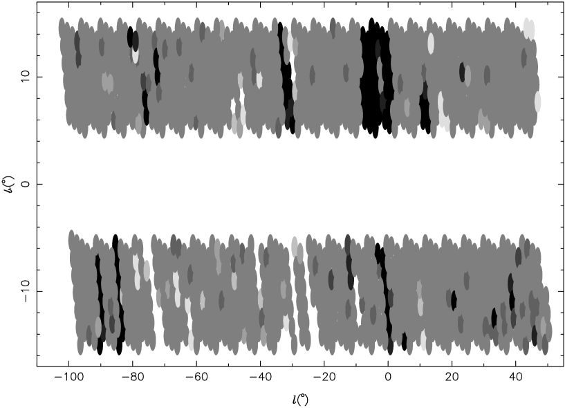
Figure 2: Sky coverage for the survey. Ellipses represent groups of four inter-meshed pointings. Shades of grey represent the density of coverage, from unobserved (white) to observed twice (black).

In 1997 the Australia Telescope National Facility commissioned a new 21-cm 13-feed multibeam receiver, primarily for HI surveys  (?; ?). The large instantaneous sky coverage and excellent sensitivity also makes the system a powerful pulsar survey instrument and this led to the commencement of a long-running deep survey of the southern Galactic plane ($|b|<5\degr$) which is expected to almost double the known population  (?; ?). We conducted Monte Carlo simulations similar to those discussed by ? and found that a shallower ‘flanking’ survey should discover a sizeable population of pulsars with unprecedented time efficiency in an area of sky not previously sampled at high frequencies. Based on this result we conducted such a survey between 1998 August and 1999 August. The survey proved highly successful, discovering 69 pulsars including two pulsar binaries containing heavy CO white dwarfs, one of which will coalesce in less than a Hubble time with dramatic and unknown consequences  (?), and a further four binary and two (perhaps three) isolated recycled pulsars with important implications for theories of binary evolution  (?). In this paper we report in detail on the observing system, analysis procedures, sensitivity and completeness. We discuss detections of previously known pulsars and present the new sample of slow pulsars, including timing results for those with solutions.

2 Observations and Analysis

2.1 Hardware Configuration and Survey Observations

The 64-m Parkes radio telescope was used with the 13-beam 21-cm receiver  (?) which provides 300 MHz of bandwidth and a system temperature of $\sim$21 K. Signals from the two orthogonal polarisations of each beam were mixed with a local oscillator before being fed to an array of 26 96-channel filterbanks. Each filterbank channel was 3 MHz wide and the band was centred at a frequency of 1374 MHz. The detected signals from corresponding polarisation pairs in each channel were summed and high pass filtered (with a time constant of $\sim$0.9 s; ?) before being integrated and one-bit sampled every 125 $\mu$s. The data stream was written to magnetic tape (DLT 7000) for offline processing, as well as being made available to online interference monitoring software in near-real-time via the computer network. With the exception of the sampling interval, the system was identical to that used for the Galactic plane survey  (?).

The receiver feeds are arranged in such a way as to allow coverage of the sky in a hexagonal grid, with beams overlapping at their approximate half-power points (7′ from the beam centre). A group of four pointings results in the uniform coverage of a roughly circular shape $\sim 1$ degree in radius which in turn can be efficiently tessellated (see Figure 1). The region enclosed by $5\degr<|b|<15\degr$ and $-100\degr<l<50\degr$ was covered in 4,764 265-s proposed pointings, amounting to only 14.6 days of integration time. Most of these pointings were observed in several week-long observing runs between August 1998 and August 1999.

2.2 Search Analysis Procedure

The processing of the 64-tape $\sim 1.6$ terabyte data set was performed on the Swinburne Supercluster, a network of 64 Compaq Alpha workstations. Before searching for pulsars, each beam was analysed for the presence of powerful signals that appeared in only a few filterbank channels, a common type of interference signal. When such signals were present, samples in the culprit channels were zeroed, a process that does not incur too much loss of sensitivity since this varies as the square root of the effective bandwidth. In addition, broad-band periodic signals that appear in large numbers of beams in any given 30-minute period were detected and logged to a file for later reference.

To correct for the effects of non-linearity in the dispersion relation, data from the 96 filterbank channels were padded with 32 dummy channels in such a way as to allow linear de-dispersion of the resulting 128 channels, as used by the Galactic plane survey collaboration. This enabled the use of the fast ‘tree’ algorithm of ? to partially de-disperse the data into eight trial dispersion measures in each of sixteen sub-bands. Whilst the linearity of dispersion with respect to channel number would enable full de-dispersion (that is, 128 trial DMs with no sub-band divisions), in order to limit storage requirements and to allow the recording of frequency-resolved pulse profiles to aid in suspect scrutiny, application of the algorithm was stopped after the production of eight DMs.

The tree algorithm produces trial DMs up to the ‘diagonal’ DM of $17.0$ cm^-3 pc, where the dispersion delay across one sub-band in units of samples is equal to the number of channels used to form it. It should be noted that in previous surveys where the linear dispersion approximation was acceptable for the tree stage, this parameter was approximately equal to the DM at which the smearing induced in each channel was one sample interval. The latter parameter is commonly quoted in conjunction with the sampling interval to give an indication of the time resolution available to pulsars of various DMs in a pulsar survey. For the present survey this value varies from $9.4$ to $17.5$ cm^-3 pc depending on the centre frequency of the channel, and for evaluation purposes one should use the geometric mean of $13.4$ cm^-3 pc. The tree algorithm was extended to also produce time series for 1–2 times the diagonal DM, and beyond this value the sample interval was doubled by summing of samples before re-application of the algorithm, and the process repeated to produce time series with 2–4, 4–8, 8–16 and 16–32 times the diagonal DM.

The periodicity search itself was based on that of the Parkes Southern Pulsar Survey  (?), generalized and modified to handle the large number of spurious interference signals present in the multibeam data. Time series were constructed at 375 trial values of dispersion measure from 0 to $562.5$ cm^-3 pc by summing partially de-dispersed sub-bands in the nearest DM with the appropriate time offsets. The trial DMs were spaced in such a way that the effective smearing induced due to the difference between the DM of a pulsar and the nearest trial DM was no more than twice that induced by the finite width of individual filterbank channels. The time series were filtered with a boxcar of width 2048 ms to remove the effects of receiver noise and gain variations during the course of the observation, before being Fourier transformed and detected to form the fluctuation power spectrum.

For signals with frequencies lying on the boundary between two spectral bins the result is two components of equal magnitude and opposite sign in the adjacent bins. To maintain sensitivity to such signals we also computed the difference of each bin and its neighbours and used half the squared magnitude of the results as alternative estimates of spectral power. For each bin the highest of the three power values computed was chosen for use in the final power spectrum. In the case of the zero-DM time series, this spectrum was checked for the occurrence of any signal with a frequency close to one earlier logged as a broad band interference signal contemporaneous with this observation. Should such a signal be present, its exact extent in the spectrum was assessed and the corresponding bins zeroed in this and all other power spectra searched in this beam. The spectrum above a frequency of $1/12$ Hz was then searched for significant spikes compared to a local mean (to compensate for the overall redness of the spectrum). Harmonics were summed and the process repeated for up to 16 harmonics to maintain sensitivity to signals with short duty cycles. Significant signals at any level of harmonic summing were recorded and after all trial dispersion measures had been searched the set of signals was correlated into a number of candidates, each covering signals of similar pulse period occurring at multiple trial DMs. The top 99 candidates in each beam were subject to a fine search (by means of maximisation of signal to noise ratio, S/N) in period and dispersion measure around the best values found in the spectral search. Pertinent information including the resulting best profile, grey scale maps of pulse profiles as a function of time and radio frequency and of signal to noise as a function of period and dispersion measure were saved to disk.

2.3 Suspect Scrutiny, Confirmation and Timing Observations

The final stage of analysis was human viewing. The large number of beams and the prevalence of interference signals presented considerable complications to the viewing process due to the volume of candidates produced. In previous surveys (e.g. ?) candidates of similar period occurring in multiple beams contemporaneously were generally taken as interference signals and ignored. In the case of results from this survey, the plethora of interference signals across the spectrum resulted in the misinterpretation of many pulsars as interference. It was found that this limited the applicability of this approach to the handful of periods that appeared more than $\sim 250$ times on any tape. All remaining candidates with signal to noise ratios greater than eight (of which there were several hundred thousand) were then scrutinized by a human viewer and promising signals scheduled for confirmation by re-observation.

Figure 3: Estimated minimum detectable mean flux density ($S_{\rm min}$) as a function of pulse period for intrinsic pulse widths of $10\degr$ (solid lines) and $90\degr$ (dashed lines) at dispersion measures of 0, 10, 30, 100 and 300 cm^-3 pc (in order of increasing $S_{\rm min}$ for a given pulse period). Points represent undetected pulsars which lie within $10\arcmin$ of an observed beam, where flux density measurements have been published. Flux densities published without uncertainties are plotted without error bars and in such cases the relative uncertainty is probably around 50 per cent.

Figure 4: Histograms depicting distribution in flux density of all previously known pulsars with published flux density with processed beams centred less than 10$\arcmin$ away. The subset of such pulsars that were undetected in the survey is represented by the hatched regions.

Table 1: Detected previously known pulsars

Name	$P$	DM	$S_{1400}$	$l$	$b$	$\Delta$ pos	S/N
	(s)	(cm-3 pc)	(mJy)	(°)	(°)	(′)
B0743–53	0.215	121.5		$-93.3$	$-14.3$	7.3	85.7
B0808–47	0.547	228.3	3.00	$-96.7$	$-8.0$		46.4
B0839–53	0.721	156.5	2.00	$-89.2$	$-7.1$	5.2	55.1
B0855–61	0.963	95		$-81.4$	$-10.4$	4.2	20.6
B0901–63	0.660	76		$-79.6$	$-11.1$	8.7	25.2
B0950–38	1.374	167		$-91.3$	$12.0$	8.2	12.9
B0957–47	0.670	92.3		$-84.3$	$5.4$	5.2	34.7
B1001–47	0.307	98.5		$-84.0$	$6.1$	2.9	31.4
J1036–4926	0.510	136.5		$-78.5$	$7.7$	5.8	10.8
J1045–4509	0.007	58.1	3.00	$-79.1$	$12.3$	0.0	37.6
J1047–6709	0.198	116.2	4.00	$-68.7$	$-7.1$	3.6	87.0
B1055–52	0.197	30.1		$-74.0$	$6.6$		51.0
B1110–65	0.334	249.1		$-66.8$	$-5.2$	5.2	38.1
B1110–69	0.820	148.4		$-65.6$	$-8.2$	5.0	18.1
B1119–54	0.536	205.1		$-69.9$	$5.9$	4.2	44.7
J1123–4844	0.245	92.9		$-71.7$	$11.6$	6.7	36.1
J1126–6942	0.579	55.3		$-64.4$	$-8.0$	3.3	15.9
B1133–55	0.365	85.2	4.00	$-67.7$	$5.9$	5.6	100.7
J1210–5559	0.280	174.3	2.10	$-62.9$	$6.4$	7.4	33.1
B1232–55	0.638	100	1.00	$-59.4$	$7.5$	19.2	22.7
B1236–68	1.302	94.1		$-58.1$	$-5.7$	11.1	32.7
B1309–53	0.728	133		$-54.0$	$8.7$	2.2	20.3
B1309–55	0.849	135.1		$-54.0$	$7.5$	0.8	102.4
B1317–53	0.280	97.6		$-52.7$	$8.6$	4.8	43.2
B1325–49	1.479	118		$-50.9$	$13.1$	6.1	17.1
J1350–5115	0.296	90.4		$-47.8$	$10.5$	4.9	25.1
B1352–51	0.644	112.1		$-47.0$	$9.7$	3.2	40.9
B1359–51	1.380	39		$-45.9$	$9.9$	63.7	71.0
J1403–7646‡	1.306	100.6		$-52.9$	$-14.5$	2.2	14.5
B1417–54	0.936	129.6		$-44.2$	$6.4$	6.1	30.7
B1426–66	0.785	65.3	6.00	$-47.3$	$-5.4$	6.7	126.2
B1451–68	0.263	8.7	80.00	$-46.1$	$-8.5$	7.0	242.9
B1454–51	1.748	35.1		$-37.9$	$6.7$	4.4	27.1
B1503–66	0.356	129.8		$-44.1$	$-7.3$	1.9	66.5
B1504–43	0.287	48.7		$-32.7$	$12.5$	4.4	107.5
B1507–44	0.944	84		$-32.4$	$11.7$		53.1
B1510–48	0.455	49.3		$-34.1$	$7.8$	5.9	16.3
B1524–39	2.418	46.8		$-27.0$	$14.0$	6.7	37.5
B1556–44	0.257	56.3	40.00	$-25.5$	$6.4$	7.0	71.3
J1557–4258	0.329	144.5	5.10	$-24.7$	$8.0$	5.6	59.5
J1603–7202	0.015	38.1	2.9(2)	$-43.4$	$-14.5$	3.6	16.1
J1614–3937	0.407	152.4		$-20.0$	$8.2$	6.1	11.7
B1620–42†	0.365	295	2.20	$-21.1$	$4.6$	13.8	12.5
J1625–4048	2.355	145		$-19.4$	$5.9$	8.1	16.1
B1630–59	0.529	134.9		$-32.3$	$-8.3$	1.5	50.9
B1641–68	1.786	43	2.00	$-38.2$	$-14.8$	4.6	110.7
B1647–52	0.635	179.1	2.00	$-25.0$	$-5.2$	4.0	117.2
B1647–528	0.891	164		$-25.4$	$-5.5$	5.8	64.1
J1648–3256	0.719	128.3	1.00	$-10.4$	$7.7$	5.5	21.0
B1649–23	1.704	68.3	1.10	$-2.7$	$12.5$		38.0
† — Pulsar lies outside nominal survey region
‡ — Pulsar originally published with incorrect period; corrected period listed

Table 2: continued

Name	$P$	DM	$S_{1400}$	$l$	$b$	$\Delta$ pos	S/N
	(s)	(cm-3 pc)	(mJy)	(°)	(°)	(′)
B1700–18	0.804	48.3	0.7(2)	$3.2$	$13.6$	6.4	18.2
J1700–3312	1.358	166.8		$-8.9$	$5.5$	9.1	21.5
B1702–19	0.299	22.9	8(3)	$3.2$	$13.0$	7.1	56.6
B1706–16	0.653	24.9	4(2)	$5.8$	$13.7$	6.5	231.4
B1707–53	0.899	106.1		$-24.3$	$-8.5$	0.4	16.9
B1709–15	0.869	58.0	0.7(2)	$7.4$	$14.0$	4.4	15.9
B1717–16	1.566	44.9	1.1(4)	$7.4$	$11.5$	3.2	19.5
B1718–19	1.004	75.9	0.30	$4.9$	$9.7$	5.2	9.1
B1727–47	0.830	123.3	12.00	$-17.4$	$-7.7$	2.3	582.4
B1730–22	0.872	41.2	2.2(3)	$4.0$	$5.7$	5.6	64.5
J1730–2304	0.008	9.6	3.0(4)	$3.1$	$6.0$		48.7
B1732–07	0.419	73.5	1.7(2)	$17.3$	$13.3$	3.5	78.4
B1738–08	2.043	74.9	1.4(4)	$17.0$	$11.3$	4.9	91.3
B1740–13	0.405	115	0.50(10)	$12.7$	$8.2$	3.9	24.0
J1744–1134	0.004	3.1	2.0(2)	$14.8$	$9.2$	3.2	24.8
B1745–12	0.394	100.0	2.0(3)	$14.0$	$7.7$	3.8	106.1
B1747–46	0.742	20.3	10.00	$-15.0$	$-10.2$	6.5	159.0
B1758–03	0.921	117.6	0.70(10)	$23.6$	$9.3$	4.1	30.3
B1802+03	0.219	79.4		$30.4$	$11.7$	6.4	27.7
B1804–08	0.164	112.8	16(4)	$20.1$	$5.6$	5.2	260.9
J1808+00	0.425	141		$28.5$	$9.8$	8.1	21.4
J1808–0813	0.876	151.3	2.00	$20.6$	$5.8$	7.1	34.9
B1810+02	0.794	101.6	0.30	$30.7$	$9.7$	4.7	14.6
J1811+0702	0.462	54		$34.7$	$12.1$	2.2	21.0
B1813–26†	0.593	128.1		$5.2$	$-4.9$	7.8	17.9
B1813–36	0.387	94.4	2.00	$-3.2$	$-9.4$	5.4	52.4
J1817–3837‡	0.384	102.8		$-5.3$	$-10.4$	7.4	57.6
B1818–04†	0.598	84.4	8.0(6)	$25.5$	$4.7$	12.0	104.6
B1820–31	0.284	50.3	2.5(6)	$2.1$	$-8.3$	8.3	72.1
B1821+05	0.753	67.2	1.7(4)	$35.0$	$8.9$	3.3	111.9
B1822+00	0.779	54.4	0.40(10)	$30.0$	$5.9$	1.4	26.6
J1822–4209	0.457	72.5	1.50	$-8.1$	$-12.8$	6.3	16.2
B1839+09	0.381	49.1	1.70(10)	$40.1$	$6.3$	3.5	99.9
B1842+14	0.375	41.2	1.5(3)	$45.6$	$8.1$	5.2	30.5
B1845–19	4.308	18.3		$14.8$	$-8.3$	9.3	84.6
B1848+12	1.205	71	0.50(10)	$44.5$	$5.9$	5.5	21.3
B1848+13	0.346	59.0	1.4(3)	$45.0$	$6.3$	8.1	32.1
J1848–1414	0.298	134.4		$19.9$	$-5.8$	4.3	11.2
B1851–14	1.147	130.1		$20.5$	$-7.2$	9.0	24.0
J1852–2610	0.336	56.8	1.40	$9.5$	$-11.9$	0.8	36.2
B1857–26	0.612	38.1	13.0(10)	$10.3$	$-13.5$	6.8	201.6
B1900–06	0.432	195.7		$28.5$	$-5.7$	10.0	13.7
J1901–0906‡	1.782	72.7	3.10	$26.0$	$-6.4$	4.7	98.6
J1904–1224	0.751	118.2		$23.3$	$-8.5$	2.5	14.9
B1907–03	0.505	205.7	0.80	$32.3$	$-5.7$	3.6	22.1
B1911–04	0.826	89.4	4.4(5)	$31.3$	$-7.1$	4.8	233.4
B1917+00	1.272	90.7	0.8(2)	$36.5$	$-6.2$	4.6	36.7
B1923+04	1.074	101.8		$41.0$	$-5.7$	9.0	15.5
J1929+00	1.167	33		$37.7$	$-8.3$	2.3	14.0
J1938+0652	1.122	70		$44.4$	$-7.1$	3.8	29.2
B1942–00	1.046	58.1	0.80(10)	$38.6$	$-12.3$	6.2	21.5
† — Pulsar lies outside nominal survey region
‡ — Pulsar originally published with incorrect period; corrected period listed

Table 3: Undetected previously known pulsars

Name	$P$	DM	$S_{1400}$	$l$	$b$	$\Delta$ pos
	(s)	(cm-3 pc)	(mJy)	(°)	(°)	(′)
B0923–58	0.740	57.7		$-81.6$	$-5.6$	15.7
J1006–6311	0.836	196.0		$-74.4$	$-6.0$	21.6
J1123–6651	0.233	111.2	0.50	$-65.5$	$-5.4$	5.4
J1130–6807	0.256	148.7		$-64.5$	$-6.4$	5.8
J1137–6700	0.556	228.0	1.10	$-64.2$	$-5.2$	17.7
J1143–5158	0.676	159.0	0.30	$-67.6$	$9.5$	3.4
J1225–5556	1.018	125.8	0.40	$-60.7$	$6.7$	6.6
J1356–5521	0.507	174.2	1.50	$-47.8$	$6.3$	11.8
B1503–51	0.841	61.0		$-36.9$	$5.5$	8.4
J1604–7203	0.341	54.4		$-43.3$	$-14.6$	4.1
J1654–2713	0.792	92.4	0.10	$-5.0$	$10.3$	3.1
B1659–60	0.306	54		$-30.2$	$-11.4$	6.3
B1700–32	1.212	109.6	6.00	$-8.2$	$5.4$	21.0
J1701–3006	0.005	115.6		$-6.4$	$7.3$	6.6
J1732–1930	0.484	73.0	0.30	$6.4$	$7.6$	5.3
B1740–03	0.445	30.2	0.50	$21.6$	$13.4$	5.0
J1740–5340	0.004	71.9		$-21.8$	$-12.0$	3.7
B1745–56	1.332	58		$-23.4$	$-14.3$	50.1
B1802–07	0.023	186.4	0.60	$20.8$	$6.8$	7.6
J1807+07	0.464	89		$35.1$	$13.3$	4.1
J1809–3547	0.860	193.8		$-3.5$	$-7.8$	7.6
B1820–30A	0.005	86.8	0.72(2)	$2.8$	$-7.9$	6.6
B1820–30B	0.379	87.0	0.07(3)	$2.8$	$-7.9$	6.6
J1821+17	1.366	79		$45.3$	$14.2$	8.7
B1821–24	0.003	119.8	1.80	$7.8$	$-5.6$	6.4
J1822+0705	1.363	50		$36.0$	$9.7$	4.2
J1822+11	1.787	112		$39.9$	$11.6$	7.4
J1823–0154	0.760	135.9	0.80	$28.1$	$5.3$	28.7
J1834+10	1.173	62		$40.6$	$8.6$	8.5
J1838+06	1.122	70		$37.5$	$6.1$	4.0
J1838+16	1.902	36		$46.7$	$10.3$	10.2
J1859+1526	0.934	97.4		$47.6$	$5.2$	76.0
J1911–1114	0.004	31.0	0.70(10)	$25.1$	$-9.6$	6.2
J1933+07	0.437	170		$44.8$	$-5.6$	10.2
J1941+1026	0.905	138.9		$48.0$	$-6.2$	15.9
J1947+10	1.111	149		$49.0$	$-7.3$	56.5
J1950+05	0.456	71		$44.9$	$-10.6$	5.5

Human viewing of all suspects with S/N $>$ 8 was expected to be incomplete in its selection due to the viewing speed necessitated by the large number of candidates to be assessed. This method was used as a first pass over the data, however after all data were processed and the 30 GB result set assembled, a more complete candidate analysis scheme was employed. A custom-written graphical software package allowed for visual (and numerical) identification of the distribution of candidates in a variety of parameters. Sets of candidates could be trimmed by the graphical or command-driven selection and deletion of interference signals, and the remaining candidate list subjected to human scrutiny. A set of ‘macros’ were developed for the deletion of dozens of commonly appearing highly coherent interference periods as well as all signals with large relative errors in dispersion measure (a characteristic of terrestrial, non-dispersed interference) and any candidate with a S/N less than 9 (or 9.5 for $P<20$ ms). These produced an order of magnitude reduction in the number of suspects to be viewed, and a corresponding improvement in the accuracy and completeness of scrutiny. Interference mitigation procedures employed for each tape were also recorded as macros to allow for repeatability and quantification of any selection effects imposed.

Those candidates confirmed by detection in a re-observation were added to an ongoing program of pulsar timing of new discoveries. Observations of typically 250 s were made with the centre beam of the system described above, or more recently the $2\times 512\times 0.5$-MHz filterbank to provide improved time resolution for short period pulsars. For most pulsars at least one timing observation was obtained at a frequency of 660 MHz to enable accurate measurement of the dispersion measure. In offline processing samples were de-dispersed and folded at the predicted topocentric pulse period. The resulting pulse profiles were fitted to a ‘standard’ profile usually produced by adding several prior observations of high signal to noise ratio. The resulting phase offsets were used to produce barycentric times-of-arrival (TOAs) which were then used in conjunction with the TEMPO software package to fit for the relevant spin, astrometric and binary parameters (see e.g. ?).

Figure 5: Pulse profiles for new slow pulsars

Figure 6: continued

3 Results and Discussion

3.1 Sky Coverage, Sensitivity and Re-Detections

The survey was deemed complete in August 1999 after the observation and successful processing of 60,852 beams in 4,702 pointings. In the first observing run an error in the telescope control system resulted in spurious rotations of the receiver feed, making the sky position corresponding to each recorded beam (except the centre beam) indeterminate and reducing sensitivity by moving off (or on!) source midway through observations. For this reason most of the region of sky surveyed under these conditions were re-observed.

Figure 2 shows the sky coverage achieved by the survey. One ellipse is plotted for each group of four inter-meshing pointings. Ellipses are shaded according to the number of observed and processed pointings in the group. Most groups are either medium grey (for standard once-only coverage), black (for those areas observed twice due to position uncertainty as discussed above) or white (for unobserved groups). Other shades reflect varying numbers of observed and processed beams in the group. A total of 4,465 of the proposed pointings were observed at least once, yielding a metric of completeness of 4,465$/$4,764 $=$ 94 per cent.

Figure 7: Distribution in pulse period and period derivative of new pulsars (stars),previously known pulsars in the survey region (large dots) and all other known pulsars (small dots), where such values have been measured. Also plotted are solid and dashed lines of constant characteristic age ($\tau_{c}\equiv P/2\dot{P}$) and inferred surface magnetic field strength ($B=3.2\times 10^{19}$ G s${}^{-1/2}\sqrt{P\dot{P}}$) respectively.

The sensitivity of a pulsar survey is derived from the radiometer equation, altered to take into account the detection of periodic signals. It can be expressed as follows,

$$S_{\rm min}=\frac{\alpha\beta(T_{\rm rec}+T_{\rm sky})}{G(N_{\rm p}\Delta\nu t_{\rm obs})^{1/2}}\left(\frac{\delta}{1-\delta}\right)^{1/2}$$ (1)

where $S_{\rm min}$ is the minimum detectable mean flux density, $\alpha$ is the threshold S/N, $\beta$ is a dimensionless correction factor for system losses, $T_{\rm rec}$ and $T_{\rm sky}$ are the receiver and sky noise temperatures, $G$ is the telescope gain, $N_{\rm p}$ is the number of polarisations, $\Delta\nu$ is the observing bandwidth, $t_{\rm obs}$ is the integration time, $W$ is the effective pulse width in time units and $P$ is the pulse period  (?). The effective pulse width ($W=\delta P$ where $\delta$ is the observed duty cycle) is computed as the quadrature sum of the intrinsic pulse width and pulse broadening terms due to such effects as dispersion smearing, scatter-broadening and the finite sampling interval.

The system characteristics of the multibeam receiver vary from beam to beam and we use here averages of the values presented at the instrument web page, yielding a receiver temperature of 21 K and a gain of 0.64 K Jy^-1. The dimensionless parameter $\beta$ embodies the loss due to one-bit digitisation ($\sqrt{\pi/2}\simeq 1.25$) and other system losses, which we treat collectively with $\beta=1.5$. Assuming a typical sky temperature of 2 K, the calculated sensitivity as a function of pulse period is plotted in Figure 3 for several dispersion measures and pulse widths. Included in the effective width calculation are the dispersion smearing in filterbank channels and the sampling interval. It should be noted that the sensitivity derived is that available at the centre of the beam. The average beam response is approximately Gaussian  (?) with a half-power width of 14.3′, meaning that pulsars lying near the beam overlap points will be detected with half the sensitivity calculated. We calculate that the mean sensitivity within the half-power radius is 73 per cent of that at the centre of the beam, meaning that for statistical sensitivity estimates, the curves in Figure 3 should be raised about a tenth of a decade. The resulting basic mean sensitivity to slow pulsars is 0.3–1.1 mJy for intrinsic pulse widths of 10°–90°.

The signal-to-noise ratio used in the sensitivity equation is calculated in the time domain. We note that some pulsar surveys (e.g. ?; ?) have based their sensitivity analysis on the so-called ‘spectral’ S/N, computed from the amplitudes of harmonics in the power spectrum. Our search code computes such a value for all candidates, however this is used only for the selection of signals to be subjected to a fine search in the time domain, and the threshold value used (5.0) is sufficiently low that we expect no loss of significant candidates at this stage. The (time domain) S/N threshold of 8.0 imposed in the selection of candidates for human viewing is also irrelevant for the sensitivity analysis since it found that nearly all candidates re-detected in subsequent observations had S/Ns greater than 10.0, despite attempts to re-detect large numbers of candidates with S/N between 8.0 and 10.0. We therefore use $\alpha=10.0$ in the above analysis and in the curves plotted in Figure 3.

We caution that this analysis should only be taken as approximate. The variation of a pulsar’s flux due to scintillation adds a considerable degree of uncertainty to its detectability, and particularly for millisecond pulsars lack of time resolution and prevalence of interference signals cause the human viewer to effectively adopt a higher threshold S/N. In particular, whilst this analysis suggests that this and similar surveys could be significantly sensitive to sub-millisecond pulsars, we would treat such a claim with skepticism. A sub-millisecond pulsar with $P=0.8$ ms and a moderately low dispersion measure of 25 cm^-3 pc would experience $0.25$ ms of dispersion smearing, resulting in a pulse profile with a width of at least $110\degr$. Combined with the fact that only 4 or perhaps 8 bins would be present in the pulse profile, the human viewer is forced to judge the origin of the signal essentially entirely upon the reported S/N, which itself becomes subject to significant uncertainty when the number of bins is so few. We therefore expect that the standard sensitivity analysis underestimates the minimum detectable flux density by a factor of a few for pulsars with periods shorter than a millisecond. Likewise, the minimum detectable flux density may be underestimated for very slow ($P>5$ s) pulsars due to the rather short time constant (0.9 s) employed in the digitiser system. The $P^{-1/2}$ duty cycle dependence of slow pulsars (e.g. ?) aids the situation somewhat, but nevertheless it is expected that a few percent of very slow pulsars have pulse widths greater than 0.5 s, and these would experience significant S/N loss.

Table 4: Dispersion measure, astrometric and spin parameters for new slow pulsars

Name	$\alpha$ (J2000)	$\delta$ (J2000)	$P$	$P$ Epoch	$\dot{P}$	DM
			(s)	(MJD)	($10^{-15}$)	(cm-3 pc)
J0834–60	08h34m50(40)	–60°35(5)′	$0.384645$(6)	51401.1	…	$20$(6)
J0843–5022	08h43m09$\aas@@fstack{s}$884(8)	–50°22′43$\aas@@fstack{\prime\prime}$10(8)	$0.2089556931527$(14)	51500.0	$0.17238$(14)	$178.47$(9)
J0849–6322	08h49m42$\aas@@fstack{s}$59(2)	–63°22′35$\aas@@fstack{\prime\prime}$0(1)	$0.367953256307$(5)	51500.0	$0.7908$(5)	$91.29$(9)
J0932–3217	09h32m39$\aas@@fstack{s}$15(6)	–32°17′14$\aas@@fstack{\prime\prime}$2(8)	$1.93162674308$(19)	51500.0	$0.250$(15)	$102.1$(8)
J0934–4154	09h34m58$\aas@@fstack{s}$20(3)	–41°54′19$\aas@@fstack{\prime\prime}$5(3)	$0.570409236430$(14)	51650.0	$0.269$(3)	$113.79$(16)
J1055–6905	10h55m44$\aas@@fstack{s}$71(9)	–69°05′11$\aas@@fstack{\prime\prime}$4(4)	$2.9193969868$(3)	51500.0	$20.336$(15)	$142.8$(4)
J1057–47	10h57m45(30)	–47°57(5)′	$0.62830$(3)	50989.1	…	$60$(8)
J1204–6843	12h04m36$\aas@@fstack{s}$72(1)	–68°43′17$\aas@@fstack{\prime\prime}$19(8)	$0.3088608620097$(19)	51500.0	$0.21708$(19)	$133.93$(9)
J1215–5328	12h15m00$\aas@@fstack{s}$62(7)	–53°28′31$\aas@@fstack{\prime\prime}$6(7)	$0.63641413680$(5)	51500.0	$0.115$(4)	$163.0$(5)
J1231–47	12h31m40(30)	–47°46(5)′	$1.8732$(3)	51200.8	…	$31$(30)
J1236–5033	12h36m59$\aas@@fstack{s}$15(1)	–50°33′36$\aas@@fstack{\prime\prime}$3(1)	$0.294759771191$(4)	51500.0	$0.1556$(4)	$105.02$(11)
J1244–5053	12h44m11$\aas@@fstack{s}$48(1)	–50°53′20$\aas@@fstack{\prime\prime}$6(1)	$0.275207111323$(4)	51500.0	$0.9998$(4)	$109.95$(12)
J1352–6803	13h52m34$\aas@@fstack{s}$45(4)	–68°03′37$\aas@@fstack{\prime\prime}$1(4)	$0.628902546380$(16)	51650.0	$1.234$(3)	$214.6$(2)
J1410–7404	14h10m07$\aas@@fstack{s}$370(5)	–74°04′53$\aas@@fstack{\prime\prime}$32(2)	$0.2787294436271$(15)	51460.0	$0.00674$(9)	$54.24$(6)
J1414–6802	14h14m25$\aas@@fstack{s}$7(1)	–68°02′58(1)″	$4.6301880619$(4)	51650.0	$6.39$(7)	$153.5$(6)
J1415–66	14h15m25(50)	–66°19(5)′	$0.392480$(10)	51396.2	…	$261$(6)
J1424–69	14h24m15(60)	–69°56(5)′	$0.333415$(8)	51309.7	…	$123$(4)
J1517–4356	15h17m27$\aas@@fstack{s}$34(1)	–43°56′17$\aas@@fstack{\prime\prime}$9(2)	$0.650836871901$(6)	51500.0	$0.2155$(6)	$87.78$(12)
J1528–4109	15h28m08$\aas@@fstack{s}$033(8)	–41°09′28$\aas@@fstack{\prime\prime}$8(2)	$0.526556139140$(4)	51500.0	$0.3955$(4)	$89.50$(10)
J1531–4012	15h31m08$\aas@@fstack{s}$05(1)	–40°12′30$\aas@@fstack{\prime\prime}$9(4)	$0.356849312855$(6)	51500.0	$0.0963$(6)	$106.65$(12)
J1535–4114	15h35m17$\aas@@fstack{s}$07(1)	–41°14′03$\aas@@fstack{\prime\prime}$1(3)	$0.432866133845$(6)	51500.0	$4.0705$(6)	$66.28$(14)
J1536–44	15h36m15(30)	–44°16(5)′	$0.46842$(6)	51063.2	…	$110$(30)
J1537–49	15h37m30(30)	–49°09(5)′	$0.301313$(6)	51402.3	…	$65$(4)
J1540–63	15h40m20(40)	–63°24(5)′	$1.63080$(16)	51307.7	…	$160$(20)
J1603–3539	16h03m53$\aas@@fstack{s}$697(5)	–35°39′57$\aas@@fstack{\prime\prime}$1(3)	$0.1419085889640$(9)	51650.0	$0.12425$(17)	$77.5$(4)
J1617–4216	16h17m23$\aas@@fstack{s}$38(5)	–42°16′59(1)″	$3.42846630955$(13)	51500.0	$18.129$(15)	$163.6$(5)
J1641–2347	16h41m18$\aas@@fstack{s}$04(6)	–23°47′36(6)″	$1.091008429855$(16)	51500.0	$0.0411$(15)	$27.7$(3)
J1649–5553	16h49m31$\aas@@fstack{s}$1(1)	–55°53′40(2)″	$0.61357070436$(7)	51650.0	$1.698$(16)	$180.4$(11)
J1655–3048	16h55m24$\aas@@fstack{s}$53(2)	–30°48′42(1)″	$0.542935874228$(9)	51500.0	$0.0366$(9)	$154.3$(3)
J1701–3130	17h01m43$\aas@@fstack{s}$513(5)	–31°30′36$\aas@@fstack{\prime\prime}$7(4)	$0.2913414710251$(12)	51500.0	$0.05596$(12)	$130.73$(6)

Table 5: continued

Name	$\alpha$ (J2000)	$\delta$ (J2000)	$P$	$P$ Epoch	$\dot{P}$	DM
			(s)	(MJD)	($10^{-15}$)	(cm-3 pc)
J1706–61	17h06m40(40)	–61°11(5)′	$0.361922$(8)	51308.7	…	$78$(6)
J1712–2715	17h12m11$\aas@@fstack{s}$71(1)	–27°15′53(2)″	$0.255359660118$(3)	51500.0	$1.2793$(3)	$92.64$(13)
J1717–5800	17h17m35$\aas@@fstack{s}$65(2)	–58°00′05$\aas@@fstack{\prime\prime}$4(3)	$0.321793346869$(6)	51650.0	$0.1957$(10)	$125.22$(14)
J1721–1939	17h21m46$\aas@@fstack{s}$61(4)	–19°39′49(5)″	$0.404039751280$(15)	51500.0	$0.1283$(15)	$103$(2)
J1739–1313	17h39m57$\aas@@fstack{s}$821(6)	–13°13′18$\aas@@fstack{\prime\prime}$6(4)	$1.215697613611$(9)	51500.0	$0.0817$(9)	$58.2$(5)
J1741–2019	17h41m06$\aas@@fstack{s}$87(3)	–20°19′24(5)″	$3.90450636119$(13)	51500.0	$16.260$(13)	$74.9$(4)
J1742–4616	17h42m26$\aas@@fstack{s}$10(2)	–46°16′53$\aas@@fstack{\prime\prime}$5(4)	$0.412401047219$(7)	51650.0	$0.0338$(12)	$115.96$(14)
J1743–4212	17h43m05$\aas@@fstack{s}$223(5)	–42°12′02$\aas@@fstack{\prime\prime}$4(2)	$0.3061669878595$(16)	51650.0	$0.7834$(4)	$131.94$(5)
J1744–1610	17h44m16$\aas@@fstack{s}$534(7)	–16°10′35$\aas@@fstack{\prime\prime}$8(8)	$1.757205868816$(16)	51500.0	$2.3767$(16)	$66.67$(14)
J1745–0129	17h45m02$\aas@@fstack{s}$06(1)	–01°29′18$\aas@@fstack{\prime\prime}$1(4)	$1.045406855598$(18)	51650.0	$0.631$(4)	$90.1$(11)
J1802+0128	18h02m27$\aas@@fstack{s}$45(2)	+01°28′23$\aas@@fstack{\prime\prime}$7(4)	$0.554261603931$(10)	51650.0	$2.109$(3)	$97.97$(12)
J1805–0619	18h05m31$\aas@@fstack{s}$436(9)	–06°19′45$\aas@@fstack{\prime\prime}$4(4)	$0.454650713078$(7)	51650.0	$0.9690$(13)	$146.22$(9)
J1806+10	18h06m50(20)	+10°24(5)′	$0.484285$(15)	51259.8	…	$58$(6)
J1808–3249	18h08m04$\aas@@fstack{s}$48(2)	–32°49′34(1)″	$0.364912241765$(10)	51500.0	$7.0494$(10)	$147.37$(19)
J1809–0743	18h09m35$\aas@@fstack{s}$92(1)	–07°43′01$\aas@@fstack{\prime\prime}$4(5)	$0.313885674748$(5)	51650.0	$0.1521$(9)	$240.70$(14)
J1811–0154	18h11m19$\aas@@fstack{s}$88(3)	–01°54′30$\aas@@fstack{\prime\prime}$9(7)	$0.92494482303$(4)	51650.0	$1.608$(6)	$148.1$(3)
J1819+1305	18h19m56$\aas@@fstack{s}$22(4)	+13°05′14$\aas@@fstack{\prime\prime}$2(7)	$1.06036354400$(6)	51650.0	$0.373$(9)	$64.9$(4)
J1824–25	18h24m15(20)	–25°36(5)′	$0.223319$(3)	51067.5	…	$155$(3)
J1832–28	18h32m30(20)	–28°43(5)′	$0.199300$(3)	51064.3	…	$127$(3)
J1837+1221	18h37m07$\aas@@fstack{s}$12(4)	+12°21′54$\aas@@fstack{\prime\prime}$0(6)	$1.96353198352$(12)	51650.0	$6.200$(16)	$100.6$(4)
J1837–1837	18h37m54$\aas@@fstack{s}$25(1)	–18°37′08(2)″	$0.618357697387$(16)	51500.0	$5.4950$(12)	$100.74$(13)
J1842+1332	18h42m29$\aas@@fstack{s}$96(6)	+13°32′01$\aas@@fstack{\prime\prime}$5(9)	$0.47160357893$(3)	51650.0	$0.229$(7)	$102.5$(7)
J1848+12	18h48m30(20)	+12°50(5)′	$0.75473$(7)	51316.7	…	$139$(20)
J1855–0941	18h55m15$\aas@@fstack{s}$68(3)	–09°41′02(1)″	$0.34540115992$(4)	51500.0	$0.240$(3)	$152.2$(3)
J1857–1027	18h57m26$\aas@@fstack{s}$45(5)	–10°27′01(2)″	$3.6872190477$(3)	51650.0	$10.55$(6)	$108.9$(7)
J1901–1740	19h01m18$\aas@@fstack{s}$03(6)	–17°40′00(6)″	$1.95685759005$(16)	51500.0	$0.823$(16)	$24.4$(6)
J1919+0134	19h19m43$\aas@@fstack{s}$62(3)	+01°34′56$\aas@@fstack{\prime\prime}$5(7)	$1.60398355528$(6)	51650.0	$0.589$(11)	$191.9$(4)
J1943+0609	19h43m29$\aas@@fstack{s}$132(5)	+06°09′57$\aas@@fstack{\prime\prime}$6(1)	$0.446226281658$(3)	51650.0	$0.4659$(6)	$70.76$(6)
J1947+0915	19h47m46$\aas@@fstack{s}$22(5)	+09°15′08$\aas@@fstack{\prime\prime}$0(8)	$1.48074382424$(9)	51650.0	$0.478$(16)	$94$(4)
J1956+0838	19h56m52$\aas@@fstack{s}$26(2)	+08°38′16$\aas@@fstack{\prime\prime}$8(4)	$0.303910924347$(7)	51650.0	$0.2199$(13)	$68.2$(13)
J2007+0809	20h07m13$\aas@@fstack{s}$5(1)	+08°09′33(2)″	$0.32572436605$(5)	51650.0	$0.137$(7)	$53.9$(10)

Table 6: Detection parameters, pulse widths and derived parameters for new slow pulsars

Name	$\Delta$ pos	S/N	$w_{50}$	$w_{10}$	$l$	$b$	$d$	$|z|$	$\tau_{c}$	$B$	$\dot{E}$
	(′)		(°)	(°)	(°)	(°)	(kpc)	(kpc)	(Myr)	$(10^{12}$ G)	($10^{30}$ erg s-1)
J0834–60	…	13.9	…	…	$-83.9$	$-11.9$	$0.5$	$0.10$	…	…	…
J0843–5022	…	10.1	11.0	50.0	$-91.5$	$-4.9$	$7.7$	$0.66$	19.2	0.19	$746$
J0849–6322	3.9	13.2	7.0	166.3	$-80.6$	$-12.2$	$>8.4$	$>1.8$	7.37	0.55	$627$
J0932–3217	5.9	17.1	3.4	7.6	$-98.7$	$14.1$	$3.8$	$0.93$	122	0.70	$1.37$
J0934–4154	4.4	10.4	10.1	…	$-91.6$	$7.4$	$3.2$	$0.41$	33.5	0.40	$57.3$
J1055–6905	3.5	17.8	5.8	10.7	$-67.1$	$-8.5$	$>12$	$>1.8$	2.27	7.8	$32.3$
J1057–47	…	16.3	11.5	…	$-76.0$	$10.7$	$3.0$	$0.56$	…	…	…
J1204–6843	5.5	18.5	10.6	15.2	$-61.3$	$-6.2$	$5.7$	$0.61$	22.5	0.26	$291$
J1215–5328	8.1	12.9	22.6	…	$-62.5$	$9.0$	$>11$	$>1.8$	87.4	0.27	$17.7$
J1231–47	…	28.5	30.7	…	$-60.5$	$15.0$	$1.6$	$0.42$	…	…	…
J1236–5033	3.2	13.2	14.7	20.8	$-59.4$	$12.2$	$>8.3$	$>1.8$	30.0	0.22	$240$
J1244–5053	4.3	12.4	8.1	…	$-58.2$	$12.0$	$>8.5$	$>1.8$	4.36	0.53	$1894$
J1352–6803	3.5	32.7	16.0	188.9	$-51.4$	$-5.9$	$14$	$1.4$	8.07	0.89	$196$
J1410–7404	5.7	30.4	2.3	4.5	$-51.7$	$-12.0$	$2.1$	$0.45$	655	0.044	$12.3$
J1414–6802	2.0	27.3	7.8	14.0	$-49.4$	$-6.4$	$6.6$	$0.74$	11.5	5.5	$2.54$
J1415–66	…	26.3	6.5	…	$-48.8$	$-4.8$	$14$	$1.2$	…	…	…
J1424–69	…	13.0	3.6	…	$-49.2$	$-8.5$	$6.3$	$0.94$	…	…	…
J1517–4356	5.6	11.8	6.1	14.4	$-31.1$	$11.5$	$4.4$	$0.88$	47.8	0.38	$30.9$
J1528–4109	3.7	19.8	6.4	12.3	$-27.9$	$12.7$	$6.0$	$1.3$	21.1	0.46	$107$
J1531–4012	5.3	15.4	11.1	…	$-26.9$	$13.1$	$>7.8$	$>1.8$	58.7	0.19	$83.6$
J1535–4114	3.8	95.0	12.5	18.3	$-26.8$	$11.8$	$2.8$	$0.57$	1.68	1.3	$1981$
J1536–44	…	15.8	…	…	$-28.5$	$9.3$	$5.3$	$0.85$	…	…	…
J1537–49	…	14.5	26.3	…	$-31.3$	$5.2$	$1.7$	$0.16$	…	…	…
J1540–63	…	25.3	12.4	…	$-39.4$	$-6.5$	$7.5$	$0.84$	…	…	…
J1603–3539	4.1	13.3	30.4	…	$-18.8$	$12.5$	$3.8$	$0.83$	18.1	0.13	$1716$
J1617–4216	5.1	10.3	3.7	9.5	$-21.5$	$5.9$	$6.3$	$0.65$	3.00	8.0	$17.8$
J1641–2347	3.7	85.1	16.2	29.7	$-4.2$	$14.7$	$1.3$	$0.34$	421	0.21	$1.25$
J1649–5553	7.3	13.5	39.9	…	$-27.9$	$-7.1$	$14$	$1.7$	5.73	1.0	$290$
J1655–3048	…	32.3	57.0	72.9	$-7.8$	$7.9$	$8.6$	$1.2$	235	0.14	$9.02$
J1701–3130	5.9	26.8	11.6	23.5	$-7.5$	$6.4$	$4.5$	$0.50$	82.5	0.13	$89.3$

Table 7: continued

Name	$\Delta$ pos	S/N	$w_{50}$	$w_{10}$	$l$	$b$	$d$	$|z|$	$\tau_{c}$	$B$	$\dot{E}$
	(′)		(°)	(°)	(°)	(°)	(kpc)	(kpc)	(Myr)	$(10^{12}$ G)	($10^{30}$ erg s-1)
J1706–61	…	21.6	2.8	…	$-30.8$	$-12.1$	$3.8$	$0.80$	…	…	…
J1712–2715	1.1	41.7	46.5	90.2	$-2.7$	$7.1$	$3.1$	$0.38$	3.16	0.58	$3033$
J1717–5800	5.0	10.9	23.5	…	$-27.3$	$-11.5$	$>8.8$	$>1.8$	26.1	0.25	$232$
J1721–1939	4.6	9.7	16.9	…	$4.9$	$9.6$	$4.7$	$0.78$	49.9	0.23	$76.8$
J1739–1313	3.3	22.6	2.4	5.3	$12.8$	$9.3$	$2.0$	$0.33$	236	0.32	$1.80$
J1741–2019	6.0	59.6	11.1	13.8	$6.8$	$5.4$	$2.0$	$0.19$	3.80	8.1	$10.8$
J1742–4616	3.1	26.3	21.8	33.2	$-15.2$	$-8.5$	$5.0$	$0.74$	193	0.12	$19.0$
J1743–4212	5.2	19.6	8.6	18.8	$-11.6$	$-6.5$	$4.7$	$0.53$	6.19	0.50	$1078$
J1744–1610	…	12.8	7.4	10.2	$10.8$	$6.9$	$2.0$	$0.24$	11.7	2.1	$17.3$
J1745–0129	5.4	12.2	2.4	8.3	$23.8$	$14.0$	$>7.3$	$>1.8$	26.3	0.82	$21.8$
J1802+0128	1.9	12.5	4.1	…	$28.6$	$11.6$	$>8.8$	$>1.8$	4.16	1.1	$489$
J1805–0619	6.0	11.1	12.7	23.0	$22.0$	$7.2$	$6.7$	$0.84$	7.43	0.67	$407$
J1806+10	…	66.3	6.7	…	$37.3$	$14.6$	$4.0$	$1.0$	…	…	…
J1808–3249	2.1	40.8	13.8	20.7	$-1.0$	$-6.1$	$5.1$	$0.54$	0.82	1.6	$5727$
J1809–0743	1.3	13.0	13.8	…	$21.2$	$5.7$	$>18$	$>1.8$	32.7	0.22	$194$
J1811–0154	3.8	21.8	8.2	77.8	$26.6$	$8.0$	$9.6$	$1.3$	9.12	1.2	$80.2$
J1819+1305	5.1	14.3	21.4	…	$41.2$	$12.8$	$4.4$	$0.98$	45.0	0.64	$12.4$
J1824–25	…	15.6	9.3	…	$7.1$	$-5.9$	$5.2$	$0.53$	…	…	…
J1832–28	…	18.0	21.3	…	$5.1$	$-8.9$	$6.4$	$1.00$	…	…	…
J1837+1221	4.9	16.1	3.1	…	$42.4$	$8.7$	$6.1$	$0.93$	5.02	3.5	$32.3$
J1837–1837	4.8	11.0	5.8	11.6	$14.8$	$-5.5$	$3.0$	$0.29$	1.78	1.9	$918$
J1842+1332	3.5	33.1	72.5	…	$44.1$	$8.1$	$5.9$	$0.83$	32.6	0.33	$86.2$
J1848+12	…	17.8	51.0	…	$44.1$	$6.5$	$7.5$	$0.84$	…	…	…
J1855–0941	2.9	19.1	26.1	…	$24.7$	$-5.2$	$4.9$	$0.45$	22.8	0.29	$230$
J1857–1027	0.9	71.4	14.6	20.5	$24.3$	$-6.1$	$3.6$	$0.38$	5.54	6.3	$8.31$
J1901–1740	5.5	131.0	6.6	22.1	$18.1$	$-10.1$	$1.3$	$0.22$	37.7	1.3	$4.34$
J1919+0134	5.0	34.2	10.5	18.2	$37.6$	$-5.6$	$10$	$0.99$	43.1	0.98	$5.64$
J1943+0609	2.5	30.1	8.9	17.7	$44.5$	$-8.6$	$3.9$	$0.58$	15.2	0.46	$207$
J1947+0915	6.1	12.7	7.5	…	$47.7$	$-8.1$	$5.8$	$0.81$	49.1	0.85	$5.81$
J1956+0838	5.8	15.0	15.4	…	$48.3$	$-10.3$	$4.3$	$0.77$	21.9	0.26	$309$
J2007+0809	5.2	14.4	92.8	…	$49.2$	$-12.8$	$3.4$	$0.76$	37.7	0.21	$156$

Figure 8: Histograms depicting distribution in pulse period of new pulsars (dashed line) and previously known pulsars in the survey region (solid line).

Figure 9: Histograms depicting distribution in maximum detected signal to noise ratio (S/N) of new pulsars (dashed line) and previously known pulsars in the survey region (solid line). One new and 8 known pulsars had S/Ns greater than 120 and are not included in this plot for clarity in low S/N bins.

Figure 10: Histograms depicting distribution in dispersion measure of new pulsars (dashed line) and previously known pulsars in the survey region (solid line).

Figure 11: Histograms depicting distribution in angular displacement from the Galactic plane of new pulsars (dashed line) and previously known pulsars in the survey region (solid line).

A total of 101 previously known pulsars were re-detected in the survey. Due to the large angular extent of each of the tessellated units of four pointings, the actual survey regions are significantly non-rectangular in $l$ and $b$ (see Figure 2) and three of these pulsars actually lie outside the nominal survey region. There were 135 previously discovered pulsars in the declared region, leaving 37 undetected in the survey. Tables 1 and 3 list the detected and undetected known pulsars, including for each pulsar the period, dispersion measure, flux density at 1400 MHz (where known), position in Galactic coordinates, angular offset from the centre of the beam in which it was detected (where known, or the nearest processed beam for undetected pulsars), and the signal to noise ratio of detections. In most cases the values for period, DM and flux density derive from the works of ?, ? or ?.

From the tabulated position offsets to the nearest processed beams and given the fact that the centres of adjacent beams of the grid are spaced 14 arcminutes apart on the sky, it is clear that the reason for many of the non-detections was incomplete sky coverage. Twelve undetected pulsars lay greater than 10 arcminutes from the nearest beam, leading to an alternative completeness metric of $1-12/135=91$ per cent, (or $1-9/135=93$ per cent if the loss is offset by the three known pulsars detected outside the survey region). Of the remaining 25 non-detections, 11 have published flux densities near 1400 MHz and are plotted along with the sensitivity curves of Figure 3. Allowing for scintillation, all are compatible with having flux densities below the sensitivity limit. We therefore expect that most of those pulsars lacking flux density measurements were also below the detection threshold at the time of observation, and conclude that the search procedure was adequate and robust in its rejection of interference without significant loss of pulsars. Possible exceptions to this statement are PSR B1556–44 which was detected at 17 times its true spin frequency (probably due to proximity in period to a persistent 256-ms interference signal), and perhaps PSR J1130–6807 which has a similar pulse period but being of unknown flux density may have simply fallen below the sensitivity limit. The discovery of PSR J1712–2715 (below) with $P=255.4$ ms indicates that rough proximity to interference signals is not always problematic. The millisecond pulsar (MSP) fraction of the undetected pulsars is high, however all except J1911–1114  (?) were discovered in deep directed searches of globular clusters  (?; ?; ?) which found mainly millisecond pulsars. Figure 4 shows a histogram of flux densities for previously known pulsars of published flux density with processed beams centred less than 10$\arcmin$ away, with the distribution of non-detections hashed. As expected from the sensitivity curves shown in Figure 3, the survey was sensitive to most pulsars brighter than 1 mJy, insensitive to pulsars with $S<0.1$ mJy, and recorded a mixture of detections and non-detections in the remaining range due to scintillation and the distribution of pulse widths.

Examination of the detection parameters of previously known pulsars reveals some discrepancies with previously published results. From inspection of the position offsets of newly discovered pulsars (below, Table 6), we estimate a position uncertainty of 7′ for detections in this survey, consistent with the beam spacing. Of those detected pulsars with published positions greater than 10′ from the beam centre, two were not detected in pointings made closer to the published position. The (B1950) declinations reported for PSRs B1232–55 and B1359–51 of $-55\degr 00(10)\arcmin$ and $-51\degr 10(15)\arcmin$  (?) respectively are inconsistent with the B1950 declinations of $-54\degr 40(5)\arcmin$ and $-50\degr 06(5)\arcmin$ of the detections made in this survey. The published right ascension values have much smaller uncertainties (due to the shape of the beam of the Molonglo telescope with which they were discovered), and are consistent with our detections.

As was spectacularly illustrated with PSR J2144–3933  (?), pulsar surveys in the past have been prone to detecting pulsars with an apparent pulse frequency an integer multiple of the true frequency. We expect that this is due to the flattening of the power spectrum with a boxcar filter, the presence of interference signals of similar period, the dominance of odd harmonics in the pulse shape, or the exclusion of the fundamental as being below a cutoff frequency (as was the case for J2144–3933). We found that PSRs J1403–7646, J1817–3837 and J1901–0906  (?) actually possess periods a factor of two greater than the published values. Conversely, pulsars J1036–4926, B1110–69, B1524–39, B1556–44, B1706–16, B1709–15, B1717–16, B1718–19 and B1848+12 were erroneously re-detected with shorter pulse periods. All but one of these results were made in the early stages of processing before interference rejection had been fine-tuned to avoid accidental filtering of pulsar harmonics near interference signals. After correction for such errors and with the exception of the three pulsars listed above, all other detections were made with pulse periods consistent with previously published parameters.

3.2 Newly Discovered Pulsars

The initial viewing of the survey results and subsequent confirmation observations resulted in the discovery of 58 new pulsars, 8 of which possess short spin periods and small period derivatives indicative of recycling and have been reported elsewhere  (?; ?). The final careful review of candidates produced a further 11 slow pulsars. Data from all pulsars were folded at twice and three times the discovery period to detect any errors of the kind described in the previous section. Pulsars J1055–6905, J1517–4356, J1802+0128 and J1808–3249 were all initially discovered at half the true spin period, however J1517–4356 and J1808–3249 were later detected at the correct period in subsequent survey observations, with higher signal to noise ratio. Pulse profiles for the 61 slow pulsars discovered in the survey are presented in Figure 5. For those pulsars with a timing solution the profile arises from the summation of numerous good observations, whilst for others the profile from the single best observation made to date is provided. It should be noted that the baselines of some profiles are corrupted due to the response of the filterbank/digitiser low pass filter.

Timing solutions have been obtained for 48 slow pulsars. The data for each pulsar span 490–830 days, depending on when the candidate re-observation was made. Since all pulsars have been timed for well over a year, we were able to accurately measure positions and period derivatives, in addition to making improved measurements of periods and dispersion measures. We have not seen obvious timing noise in any pulsar, however it is possible that such noise is present and is absorbed by deviations from the “true” values of the fitted parameters. Dispersion measures were fitted for by the use of TOAs derived from sub-divisions of the observing band, or where available, 660 MHz observations. In the latter case the signal to noise ratio available in a reasonable integration time was poor and the use of an independent template profile was eschewed in favour of the superior 20-cm template.

Table 4 presents the basic parameters of the slow pulsars discovered in this survey, derived from timing measurements when available. Values in parentheses denote uncertainties in the last quoted digit and represent twice the formal uncertainty produced by TEMPO. In the case of pulsars lacking a timing solution we use twice the errors derived from the fine $P$-DM search, or for positions, errors corresponding to a randomly oriented offset of 7 arcminutes (i.e. $7\arcmin/\sqrt{2}\simeq 5\arcmin$ in each of $\alpha$ and $\delta$). PSR J1802+0128 was timed for 493 days before it was discovered that the true spin period was twice the assumed value. Values presented for $P$ and $\dot{P}$ are twice the values derived by this timing analysis and retain their prior relative errors. Due to the effects of the evolution of profile morphology with frequency and the use of the 20 cm as template for timing 50 cm observations, the formal errors presented for the dispersion measure may have been underestimated. Pulsar names are assigned from their equatorial coordinates in the J$2000.0$ equinox, with four digits of declination for those with accurate positions from timing solutions, and two digits for those without. The latter names are provisional and will be altered when accurate timing positions become available. Table 6 lists additional parameters for the newly discovered pulsars, including the best S/N of the discovery observation(s) and the pulsar’s position offset from the centre of the beam, the width of the pulse profile at 10 and 50 per cent of peak intensity, its position in Galactic coordinates, its distance and $z$-displacement from the Galactic plane under the model of ? (accurate to 30 per cent on average), and inferred parameters concerning the pulsar spin-down. These assume magnetic dipole spin-down and comprise the characteristic age ($\tau_{c}\equiv P/2\dot{P}$), surface magnetic field strength ($B=3.2\times 10^{19}$ G s${}^{-1/2}\sqrt{P\dot{P}}$) and spin-down power ($\dot{E}=4\pi^{2}I\dot{P}P^{-3}$, assuming $I=10^{45}$ g cm² for the moment of inertia of the neutron star). Both tables are accessible on the internet in machine-readable format at the Swinburne Pulsar Group home page. For several pulsars the dispersion measure is higher than that allowed in the given direction under the model of ?, and the values presented are given as lower limits. Such findings are not uncommon (e.g. ?; ?), and indicate that the model probably underestimates the scale height of the Galactic electron distribution.

The spin parameters of the newly discovered systems are similar to those of pulsars previously known in the search region. Figure 7 shows the distribution in period and period derivative of new pulsars with timing solutions and of previously known pulsars inside and outside the survey region. Both new and previously known slow pulsars in the region tend to have longer inferred characteristic ages than those outside the survey region, by simple virtue of the fact that pulsars are born near the Galactic plane and typically take several Myr to reach a $z$-height corresponding to $|b|>5\degr$ (for typical distances of several kpc). Figure 8 shows histograms of pulse period for the new and previously known population. It appears that this survey has uncovered a higher fraction of pulsars in the period range of 6–50 ms, however this effect is not highly significant : a Kolmogorov-Smirnov (K-S) test on the distributions for $P<100$ ms yields a 46 per cent probability of the two samples arising from the same parent distribution. When binary evolution considerations are taken into account and the new sample restricted to the four MSPs with probable helium companions the significance rises to 91 per cent, however due to the small sample size this result must be treated with caution  (?).

The discrepancy in the case of the slow pulsar population is more significant, with a K-S test indicating a different distribution at the 98 per cent level. The reason for the discrepancy, which is mainly seen as a deficit of pulsars with $P\simeq 1$ s, is not well understood. The problem remains (at 94 per cent significance) when the new sample is compared only to those previously known pulsars re-detected in this survey, confirming that the survey was able to detect pulsars in the period range in question. However, if there existed (by an unknown mechanism) a reduced sensitivity (or higher effective threshold signal to noise ratio) around $P\simeq 1$ s, one might expect the period distribution of the new pulsars to be more strongly affected than that of the previously known pulsars since the new population is on average of lower flux density. We note that the rejection of pulsars as mis-categorized interference signals cannot explain this result, since in this case one would expect an equal rate of rejections of new and previously known pulsars independent of signal to noise ratio or flux density. Comparison of the (yet to be measured) flux densities of new pulsars in and out of the depleted period range will help in evaluating the effective sensitivity of the survey as a function of period.

Figure 9 shows the distribution of signal to noise ratios in the best detections of new and previously known pulsars. As one would expect, most of the pulsars with high signal to noise ratios were detected in earlier surveys. A few of the new pulsars however were very strong and may have been missed in earlier surveys due to scintillation or due to an intrinsically flat spectrum. It is apparent from the histogram and from inspection of Tables 1 and 6 that the threshold signal to noise ratio for this survey is approximately 10, in contrast to the value of $8.0$ commonly used in previous surveys in assessing sensitivity. Numerous promising candidates with signal to noise ratios in the range of 8–10 were subjected to re-observation however only one was re-detected in such observations despite using longer integration times, probably because they actually arose from interference or by random chance (given the size and dimensionality of the search space).

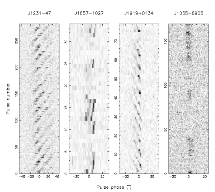
Figure 12: Greyscale plots of detected flux density as a function of pulse phase and pulse number for four newly discovered pulsars. Each row represents a single pulse.

As noted in the introduction, high frequency surveys are also expected to sample a different area of the pulsar spectral index distribution, compared to low frequency surveys. The sensitivity of the present work to a pulsar with a spectral index of $-1.7$ (typical of those discovered at 70 cm; ?) is comparable to that of the Parkes Southern Pulsar Survey  (?), the most sensitive previous 70 cm search to cover a large region of the area observed by the present study. One therefore expects the distances of the newly discovered pulsars to be comparable to the previously known population in the region, and as shown in Figure 10, this is indeed the case. The bulk of newly discovered pulsars had S/Ns $\la 30$, suggesting (in conjunction with their non-detection in the 70 cm survey) spectral indices of up to $-0.7$. Eleven newly discovered pulsars are visible from the 305-m Arecibo telescope and were presumably within the search area of previous surveys conducted there  (?; ?; ?; ?), which were typically sensitive to ($\delta=0.1$) pulsars brighter than $\sim 1$ mJy at 70 cm. Their non-detection in the Arecibo surveys suggests $\alpha\ga-1.1$. Several pulsars were discovered at high S/N, which could be indicative of positive spectral indices (for example, J1806+10 in Arecibo territory, yielding $\alpha\simeq 2.6$), however the non-detections may well be the result of incomplete surveys or interstellar scintillation.

Accurate characterization of the spectral indices of the newly discovered pulsars must await calibrated multi-frequency flux density measurements, however we note in passing that the detection of these pulsars at 660 MHz required significantly more integration time than expected for pulsars of average spectral index. As indicated by the lack of any enhanced preference for low Galactic latitudes in the newly detected sample compared to the previously known pulsars (Figure 11), reduced scatter-broadening at 20-cm in general does not appear to have been a significant factor in the discovery of the new pulsars.

3.3 Individual Pulsars of Interest

As previously reported  (?), the pulse profile of PSR J1410–7404 is exceedingly narrow and contradicts the pulse width – period relation of ?. Since all major contradictions in the past have been from apparently recycled pulsars, it is conceivable that J1410–7404 is also recycled, a hypothesis supported by the small magnetic field strength inferred from timing observations. The newly discovered pulsar J1706–61 also has a measured profile width seemingly in disagreement with ?, in this case being 70 per cent of the predicted minimum width. However, we caution that this measurement derives from a single observation of moderate signal-to-noise ratio (as visible in Figure 5) and that a more definite conclusion awaits the availability of an extended data set from ongoing timing observations. Should the improved profile maintain the narrow width derived here, the magnetic field strength and characteristic age derived from timing measurements will be of great utility in evaluating the recycling hypothesis for PSRs J1410–7404 and J1706–61.

As expected from the relatively old age of the sample detected here, numerous pulsars appear to exhibit noticeable pulse nulling (e.g. ?). Several pulsars also show drifting sub-pulses (e.g. ?) of varying degrees of regularity. Figure 12 depicts the instantaneous flux density of four newly discovered pulsars as a function of pulse phase and pulse number. It is apparent that the emission of PSRs J1231–47 and J1919+0134 is strongly modulated by sub-pulses showing very regular drift. PSR J1857–1027 also appears to show drifting sub-pulses in this and other observations, although as a result of the short duration of observations made for timing analysis, combined with the long pulse period ($\sim 3.7$ s), the number of pulses recorded and hence the conspicuousness of this effect in archival observations is reduced. Detailed analysis of these pulsars will appear in a forthcoming paper (Ord et al. in preparation).

Pulse nulling appears to occur on a wide range of time scales in the detected pulsars. The data for PSR J1231–47 in Figure 12 were recorded in a second attempt at confirmation of this pulsar, resulting in a signal to noise ratio of 82 in an observation of 530 s. Several subsequent observations of between 900 and 4000 s succeeded in producing only one further weak detection of the pulsar. PSRs J1857–1027 and J1055–6905 appear to null on more typical timescales of $\sim$1–50 pulses, as shown in Figure 12. Future observations of the candidate nulling pulsars from our sample will enable analysis similar to that of ?, which in turn will help decide whether the observed flux density variations arise due to nulling or simply as a result of interstellar scintillation.

4 Conclusions

We have conducted a survey of intermediate latitudes of the southern Galaxy for pulsars at $\sim$1400 MHz. The new 13-beam 21-cm receiver of the Parkes radio telescope was used to rapidly cover to moderate depth a large region of sky flanking the area of the deeper ongoing Galactic plane survey  (?; ?). The interference environment was formidable, however development of a comprehensive scheme for the rejection of pulsar candidates arising from interference enabled the realisation of the full expected survey sensitivity of approximately $0.5$ mJy for slow and most millisecond pulsars. The survey was highly successful, detecting 170 pulsars of which 69 were previously unknown, in a relatively short observing campaign. The new discoveries are not significantly more distant than the previously known population in this region of sky, indicating that the success of the survey is attributable to its sampling of a different portion of the broad distribution of pulsar spectral indices. The detected sample, in combination with those of the Galactic plane and high-latitude surveys (when complete), will prove invaluable for population modelling due to the use of a common observing system to cover a large area of sky at high radio frequency.

Among the most interesting new objects are two recycled pulsars with massive white dwarf companions  (?), four with probable low-mass He dwarf companions, two isolated millisecond pulsars, and one ‘slow’ pulsar with a very narrow pulse profile and small period derivative, suggestive of recycling in a scenario similar to those of the known double neutron star systems  (?). As expected from the large Galactic $z$-height of much of the survey volume, the detected population of slow pulsars was relatively old and as such exhibited a high fraction of pulsars showing nulling and sub-pulse modulation. Two pulsars show very regular drifting sub-pulses and are analysed in detail elsewhere (Ord et al. in preparation).

References

- [Ables, Komesaroff & Hamilton¡1970¿] Ables J. G., Komesaroff M. M., Hamilton P. A., 1970, Astrophys. Lett., 6, 147
- [Backer¡1973¿] Backer D. C., 1973, ApJ, 182, 245
- [Barnes et al.¡2001¿] Barnes D. G. et al., 2001, MNRAS, in press
- [Bell et al.¡1995¿] Bell J. F., Bessell M. S., Stappers B. W., Bailes M., Kaspi V. M., 1995, ApJ, 447, L117
- [Biggs et al.¡1994¿] Biggs J. D., Bailes M., Lyne A. G., Goss W. M., Fruchter A. S., 1994, MNRAS, 267, 125
- [Camilo & Nice¡1995¿] Camilo F., Nice D. J., 1995, ApJ, 445, 756
- [Camilo et al.¡1996¿] Camilo F., Nice D. J., Shrauner J. A., Taylor J. H., 1996, ApJ, 469, 819
- [Camilo et al.¡2000¿] Camilo F. et al., 2000, in Kramer M., Wex N., Wielebinski R., eds, Pulsar Astronomy - 2000 and Beyond, IAU Colloquium 177. Astronomical Society of the Pacific, San Francisco, p. 3, astro-ph/9911185
- [Camilo, Nice & Taylor¡1996¿] Camilo F., Nice D. J., Taylor J. H., 1996, ApJ, 461, 812
- [Clifton et al.¡1992¿] Clifton T. R., Lyne A. G., Jones A. W., McKenna J., Ashworth M., 1992, MNRAS, 254, 177
- [D’Amico et al.¡1998¿] D’Amico N., Stappers B. W., Bailes M., Martin C. E., Bell J. F., Lyne A. G., Manchester R. N., 1998, MNRAS, 297, 28
- [D’Amico et al.¡2001¿] D’Amico N., Lyne A. G., Manchester R. N., Possenti A., Camilo F., 2001, ApJ, 548, L171
- [Dewey et al.¡1985¿] Dewey R. J., Taylor J. H., Weisberg J. M., Stokes G. H., 1985, ApJ, 294, L25
- [Edwards & Bailes¡2001a¿] Edwards R. T., Bailes M., 2001a, ApJ, in press, astro-ph/0102026
- [Edwards & Bailes¡2001b¿] Edwards R. T., Bailes M., 2001b, ApJ, 547, L37
- [Foster et al.¡1995¿] Foster R. S., Cadwell B. J., Wolszczan A., Anderson S. B., 1995, ApJ, 454, 826
- [Henning et al.¡2000¿] Henning P. A. et al., 2000, AJ, 119, 2686
- [Johnston et al.¡1992a¿] Johnston S., Lyne A. G., Manchester R. N., Kniffen D. A., D’Amico N., Lim J., Ashworth M., 1992a, MNRAS, 255, 401
- [Johnston et al.¡1992b¿] Johnston S., Manchester R. N., Lyne A. G., Bailes M., Kaspi V. M., Qiao G., D’Amico N., 1992b, ApJ, 387, L37
- [Johnston et al.¡1993¿] Johnston S. et al., 1993, Nature, 361, 613
- [Kramer, Wex & Wielebinski¡2000¿] Kramer M., Wex N., Wielebinski R., eds, Pulsar Astronomy - 2000 and Beyond, IAU Colloquium 177, Astronomical Society of the Pacific, San Francisco, 2000
- [Lawson et al.¡1987¿] Lawson K. D., Mayer C. J., Osborne J. L., Parkinson M. L., 1987, MNRAS, 225, 307
- [Lommen et al.¡2000¿] Lommen A. N., Zepka A., Backer D. C., McLaughlin M., Cordes J. M., Arzoumanian Z., Xilouris K., 2000, ApJ, 545, 1007
- [Lorimer et al.¡1995¿] Lorimer D. R., Yates J. A., Lyne A. G., Gould D. M., 1995, MNRAS, 273, 411
- [Lorimer et al.¡1996¿] Lorimer D. R., Lyne A. G., Bailes M., Manchester R. N., D’Amico N., Stappers B. W., Johnston S., Camilo F., 1996, MNRAS, 283, 1383
- [Lyne et al.¡1987¿] Lyne A. G., Brinklow A., Middleditch J., Kulkarni S. R., Backer D. C., Clifton T. R., 1987, Nature, 328, 399
- [Lyne et al.¡1998¿] Lyne A. G. et al., 1998, MNRAS, 295, 743
- [Lyne et al.¡2000¿] Lyne A. G. et al., 2000, MNRAS, 312, 698
- [Manchester et al.¡1978¿] Manchester R. N., Lyne A. G., Taylor J. H., Durdin J. M., Large M. I., Little A. G., 1978, MNRAS, 185, 409
- [Manchester et al.¡1996¿] Manchester R. N. et al., 1996, MNRAS, 279, 1235
- [Manchester et al.¡2000¿] Manchester R. N. et al., 2000, in Kramer M., Wex N., Wielebinski R., eds, Pulsar Astronomy - 2000 and Beyond, IAU Colloquium 177. Astronomical Society of the Pacific, San Francisco, p. 49
- [Manchester et al.¡2001¿] Manchester R. N. et al., 2001, MNRAS, Submitted.
- [Rankin¡1990¿] Rankin J. M., 1990, ApJ, 352, 247
- [Ray et al.¡1996¿] Ray P. S., Thorsett S. E., Jenet F. A., van Kerkwijk M. H., Kulkarni S. R., Prince T. A., Sandhu J. S., Nice D. J., 1996, ApJ, 470, 1103
- [Ritchings¡1976¿] Ritchings R. T., 1976, MNRAS, 176, 249
- [Stappers et al.¡1996¿] Stappers B. W. et al., 1996, ApJ, 465, L119
- [Staveley-Smith et al.¡1996¿] Staveley-Smith L. et al., 1996, Proc. Astr. Soc. Aust., 13, 243
- [Taylor & Cordes¡1993¿] Taylor J. H., Cordes J. M., 1993, ApJ, 411, 674
- [Taylor & Weisberg¡1989¿] Taylor J. H., Weisberg J. M., 1989, ApJ, 345, 434
- [Taylor, Manchester & Lyne¡1993¿] Taylor J. H., Manchester R. N., Lyne A. G., 1993, ApJS, 88, 529
- [Taylor¡1974¿] Taylor J. H., 1974, A&AS, 15, 367
- [Toscano et al.¡1998¿] Toscano M., Bailes M., Manchester R., Sandhu J., 1998, ApJ, 506, 863
- [Wolszczan & Frail¡1992¿] Wolszczan A., Frail D. A., 1992, Nature, 355, 145
- [Young, Manchester & Johnston¡1999¿] Young M. D., Manchester R. N., Johnston S., 1999, Nature, 400, 848