$N$-Body Code with Adaptive Mesh Refinement

Abstract

We have developed a simulation code with the techniques which enhance both spatial and time resolution of the PM method for which the spatial resolution is restricted by the spacing of structured mesh. The adaptive mesh refinement (AMR) technique subdivides the cells which satisfy the refinement criterion recursively. The hierarchical meshes are maintained by the special data structure and are modified in accordance with the change of particle distribution. In general, as the resolution of the simulation increases, its time step must be shortened and more computational time is required to complete the simulation. Since the AMR enhances the spatial resolution locally, we reduce the time step locally also, instead of shortening it globally. For this purpose we used a technique of hierarchical time steps (HTS) which changes the time step, from particle to particle, depending on the size of the cell in which particles reside. Some test calculations show that our implementation of AMR and HTS is successful. We have performed cosmological simulation runs based on our code and found that many of halo objects have density profiles which are well fitted to the universal profile proposed by Navarro, Frenk, & White (1996) over the entire range of their radius.

1 Introduction

Simulating the formation process of galaxies in clusters and fields simultaneously is one of the promising strategies to study how statistical properties of observed galaxies have originated. For this purpose, the box size in which the simulation is performed must be larger than a typical cluster separation, which is a few tens to a hundred Mpc. At the same time, in order to reproduce the intrinsic dynamical structure of each simulated galaxy, the Newtonian gravity should be calculated on a scale well below the characteristic length of individual galaxies, which is a few kpcs. Hence, for the simulation of formation of multiple galaxies, the ratio of box size to minimum resolved scale or the spatial dynamic range must be greater than $10^{5}$.

In addition, there is another dynamic range in $N$-body systems often called the mass dynamic range, or simply, the number of particles if the mass of particles is the same. Strictly speaking, dark matter component evolves according to the collisionless Boltzmann equation. However, since computer resources are finite, the distribution function of ideal collisionless component is replaced by a finite sum of localized distribution functions corresponding to the finite number of particles in the $N$-body simulation. This causes two-body relaxation which artificially affects the evolution of dark matter distribution. The effect of relaxation can be suppressed by introducing more particles. We crudely estimate how many particles are required to trace the evolution of galactic dark halos in a cosmological simulation by comparing the relaxation time scale of dark halos and their age. Our naive estimation gives $N\sim 10^{9}$ at the minimum (see Appendix A).

It is instructive to examine whether the particle-mesh (PM) method is capable of the required spatial dynamic range of $10^{5}$ and the required mass dynamic range of $10^{9}$. The spatial dynamic range of the PM method is restricted by the mesh spacing. When the number of meshes is taken as many as the number of particles, the spatial dynamic range is about $10^{3}$ for a simulation with $10^{9}$ particles, which is two orders smaller than required. However, a simulation with $10^{15}$ meshes and particles, whose spatial dynamic range is about $10^{5}$, is not only unrealistic today, but also inefficient. The adaptive mesh refinement (AMR) is one of the prescriptions to resolve this problem by introducing finer meshes hierarchically in regions where higher spatial resolution is required (Berger & Oliger 1984).

First, Villumsen (1989) introduced cubic subgrids hierarchically into the PM method to increase its spatial resolution. While his hierarchical PM code places adaptive meshes by hand, subgrids are automatically located in the particle–multiple mesh code developed by Jessop, Duncan, & Chau (1994). Gelato, Chernoff, & Wasserman (1997) extended their methods to handle isolated $N$-body systems. Their code is applicable to non-cosmological problems. On the other hand, adopting the multigrid method as the Poisson solver, Suisalu & Saar (1995) developed a code which can treat rectangular adaptive meshes. Furthermore, Kravtsov, Klypin, & Khokhlov (1997) developed the adaptive refinement tree (ART) code which subdivides all cells which satisfy the user defined refinement criterion regardless of the shape of the boundary between coarse meshes and refined meshes.

Calculating the force between particles is the most time consuming part in $N$-body methods. In order to overcome this problem, Aarseth (1963) changed the timing to calculate the force, from particle to particle, depending on the time scale of force variation. This technique, named individual time steps is implemented in the ART code (Kravtsov et al. 1998) with modification such that the time steps of particles are determined by the local density, though not described in detail in their paper. We also adopted the modified individual time steps, or hierarchical time steps (HTS) so that our code is adaptive not only in space but also in time, or our code is four dimensionally adaptive. Furthermore, our code is designed to incorporate the hydrodynamics code with AMR (Yahagi & Yoshii 2000), similar to the codes developed by Anninos, Norman, & Clarke (1994) and Norman & Bryan (1999). While the refined regions are restricted to be rectangular parallelepipeds in their codes, this limitation has been relaxed in ours.

In §2 we review the basic equations for the cosmological $N$-body simulation and describe our code in detail putting emphasis on the parts related to AMR and HTS. Details of tests and the results are discussed in §3. Finally, we summarize this work in §4.

2 Description of the code

2.1 Basic equations

For the cosmological simulation, the comoving coordinate system is suitable to represent particle position:

$$\mbox{\boldmath{$x$}}=a^{-1}\mbox{\boldmath{$r$}},$$ (1)

where $a$ is the scale factor, and $x$ and $r$ are comoving and proper positions, respectively. However, in order to incorporate the hydrodynamics code, the proper coordinate system is suitable to represent the velocity:

$$\mbox{\boldmath{$u$}}=\frac{d\mbox{\boldmath{$r$}}}{dt}-\frac{\dot{a}}{a}\mbox{\boldmath{$r$}}.$$ (2)

Using these variables, the basic equations for $N$-body systems in the expanding universe are given by:

$$\frac{d\mbox{\boldmath{$x$}}}{dt} = \frac{1}{a}\mbox{\boldmath{$u$}},$$ (3)

$$\frac{d(a\mbox{\boldmath{$u$}})}{dt} = \mbox{\boldmath{$g$}}(\mbox{\boldmath{$x$}}),$$ (4)

$$\mbox{\boldmath{$g$}}(\mbox{\boldmath{$x$}}) = -\nabla\phi(\mbox{\boldmath{$x$}}),$$ (5)

$$\triangle\phi(\mbox{\boldmath{$x$}}) = \frac{4\pi G}{a}(\rho(\mbox{\boldmath{$x$}})-\bar{\rho}),$$ (6)

and

$$\dot{a} = H_{0}\sqrt{(1-\Omega_{0}-\lambda_{0})+a^{-1}\Omega_{0}+a^{2}\lambda_{0}}.$$ (7)

Note that $\rho$ denotes the comoving density, here. How to discretize these equations depends on the problem to be solved and the strategy for it. Since the primary objective of our code is to perform the cosmological simulation with a wide dynamic range in both space and mass, we must save memory as much as possible. Thus using the variable time-step leapfrog integrator which does not require additional memory, we discretize equations (3) and (4) as follows:

$${\mbox{\boldmath{$x$}}}_{i+1} = {\mbox{\boldmath{$x$}}}_{i}+\frac{1}{a_{i+1/2}}{\mbox{\boldmath{$u$}}}_{i+1/2}~{}\Delta t_{i},$$ (8)

$${\mbox{\boldmath{$u$}}}_{i+1/2} = \frac{a_{i-1/2}}{a_{i+1/2}}{\mbox{\boldmath{$u$}}}_{i-1/2}+\frac{1}{a_{i+1/2}}{\mbox{\boldmath{$g$}}}_{i}~{}\frac{\Delta t_{i-1}+\Delta t_{i}}{2}.$$ (9)

Among a variety of methods to solve equations (5) and (6), we adopt the mesh based method, such as the PM method, which calculates the force between particles through the following steps: (i) Mass of particles is assigned to their adjacent grid nodes. (ii) Discretized Poisson equation is solved to give the potential on each node. (iii) Force on each node is calculated as the difference of the potential on nearby nodes. (iv) Force on particles is interpolated from those on the adjacent nodes. We discuss the mass assignment (i), force interpolation (iv), and potential differentiation (iii) in §2.4, while the Poisson solver (ii) in §2.5.

2.2 Hierarchical mesh

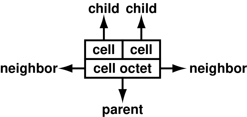
The PM method uses a cubic mesh to calculate the force on particles. Therefore, the spatial resolution of the PM method is limited by the spacing of this mesh. Like the ART code developed by Kravtsov et al. (1997), our code overcomes this limitation by subdividing the cells in regions where higher spatial resolution is required. This adaptive mesh refinement corresponds to adding data sets for small cells onto the homogeneous and cubic base mesh hierarchically. In order to maintain and modify the hierarchical mesh structure, it is required to access the parent, child, and neighbor cells. The storage for pointers to the parent and neighbor cells can be saved by grouping the cells which have the same parent cell (Khokhlov, 1998). Since one refinement process divides a cell into eight half-sized cells, we group these eight cells together and call this group a cell octet (Fig. 1). Each cell octet keeps a pointer to the parent cell and pointers to the six neighboring cell octets. In the $N$-body code, in addition to these data, a pointer to the first particle in the cell octet, the number of particles in the cell octet, and the integral position of the cell octet are also stored. The integral position is the position rounded off to integer. While cell octets residing in the same level are connected by the doubly linked lists in the ART code, our code stores the cell octets having the same level in an array consecutively. The level of a cell, $L$, is defined as $L=\log_{2}(l_{0}/l_{L})$, where $l_{0}$ and $l_{L}$ are the sizes of the simulation box and the cell, respectively. We use cells having integral level only.

Moreover, the same level cell octets are sorted by the Morton ordering (Barnes & Hut 1989; Warren & Salmon 1993). The key for the Morton ordering, $k_{M}$, is given by

$$k_{M} = \sum_{L_{i}=0}^{L_{D}}(2^{3L_{i}}k^{x}_{L_{i}}+2^{3L_{i}+1}k^{y}_{L_{i}}+2^{3L_{i}+2}k^{z}_{L_{i}}),$$ (10)

where $L_{D}$ is the level of the smallest hierarchical mesh, and $k^{x}_{L_{i}},k^{y}_{L_{i}}$, and $k^{z}_{L_{i}}$ are the $L_{i}$-th bit of the integral position of the cell octet normalized by $l_{L_{D}}$ ($\tilde{x},\tilde{y}$, and $\tilde{z}$). Thus,

$$\tilde{x} = \sum_{L_{i}=0}^{L_{D}}2^{L_{D}-L_{i}}k^{x}_{L_{i}},$$ (11)

$$\tilde{y} = \sum_{L_{i}=0}^{L_{D}}2^{L_{D}-L_{i}}k^{y}_{L_{i}},$$ (12)

$$\tilde{z} = \sum_{L_{i}=0}^{L_{D}}2^{L_{D}-L_{i}}k^{z}_{L_{i}}.$$ (13)

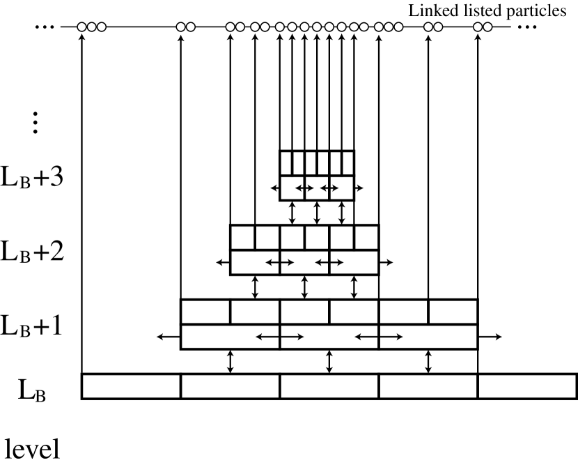
We do not sort particles as Warren and Salmon’s hashed oct-tree code (Warren & Salmon 1993), because it is incompatible with HTS, though sorting hierarchical cells is compatible with HTS. The hierarchical mesh is maintained using the cell octets as the building blocks (Fig. 2), which are added or removed from meshes freely.

Basically each cell has only one pointer to the child octet, but the storage changes depending on what physics is incorporated in the code. In the code for the self gravitating system, density and potential is stored. No additional storage is required for the $N$-body code, since the storage for a pointer to the first particle in the cell is shared by the pointer to the child cell octet. The hydrodynamics code requires storage for fluid density, specific energy and fluid velocity in each cell.

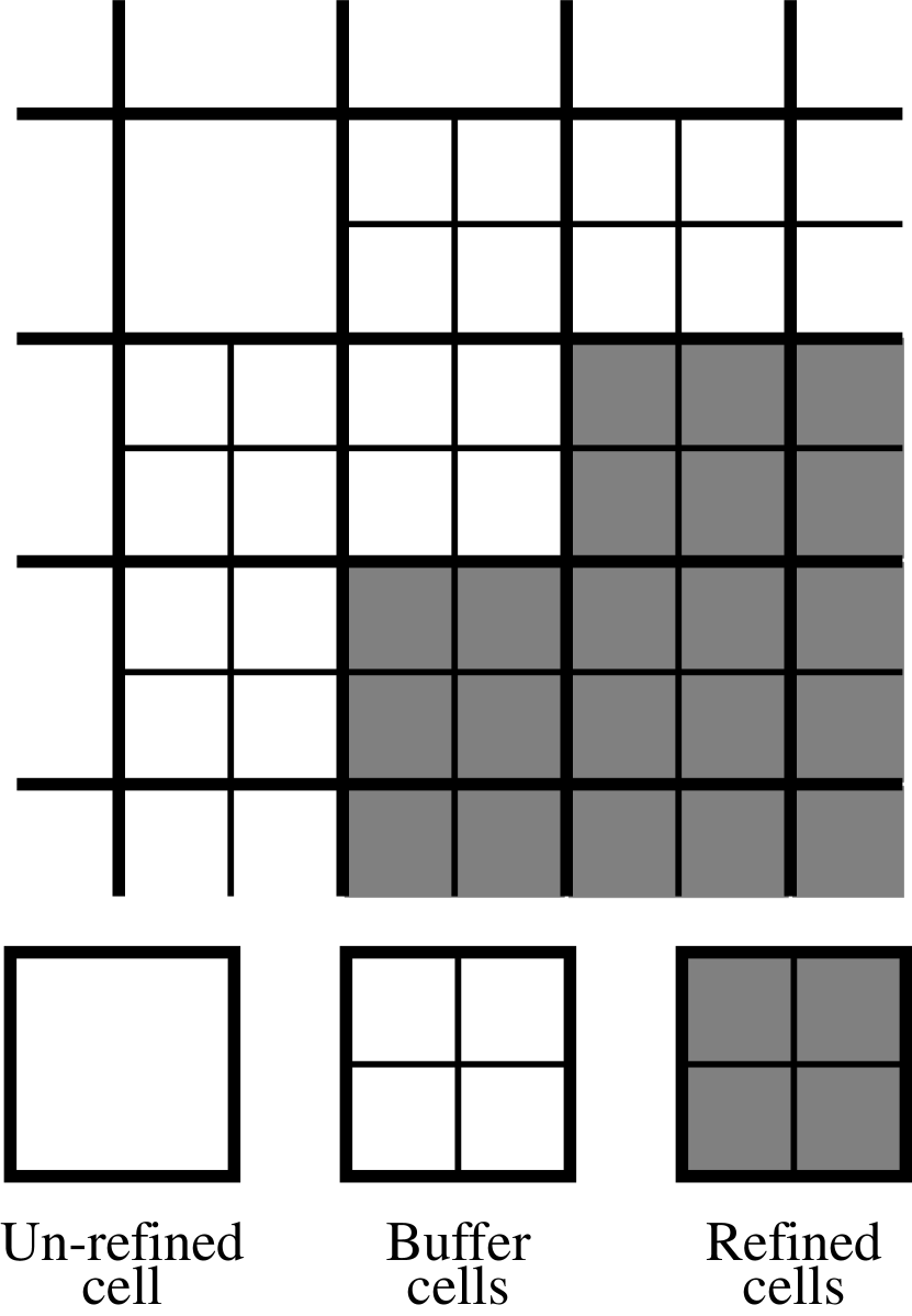
The condition for subdividing the cells, or the refinement criterion, plays an important role in the AMR. In general context of the AMR, the refinement criterion is defined using error estimators such as the residual of the partial differential equation to be solved. However, since we introduced the AMR to keep the mass dynamic range all the way from homogeneous to clustered configurations, we refined all cells which contain $N_{\mbox{\small rfn}}$ particles and more as the ART code. This criterion sets the upper limit to the mass in unrefined cells. We set $N_{\mbox{\small rfn}}=4$ throughout this paper unless otherwise stated. Following this refinement criterion, the hierarchical meshes are constructed recursively on the cubic structured mesh whose base level is $L_{B}$, until they reach the dynamic range level, $L_{D}$. At the same time, the cells which do not satisfy the refinement criterion are removed from the hierarchical meshes. In addition to the refined cells which satisfy the refinement criterion, we also subdivide those cells, named buffer cells, which are adjacent to the refined cells (Fig. 3).

For the illustrative purpose, we take an example from a slice of the cosmological simulation for an LCDM universe described in §3.4. The left panel of Figure 4 shows the distribution of particles, and the right panel shows the configuration of hierarchical meshes placed in accordance with the above prescription. While the cells including the sheet structure are refined once, more levels of hierarchical meshes are placed in the regions where massive halos reside.

2.3 Individual time steps

We adopted a time stepping scheme called the hierarchical time steps (e.g. Makino 1991). The time step of each particle is not the same but restricted to $2^{-i}$ times of the longest time steps. We chose $i$ to be the refinement level, $L-L_{B}$, (Kravtsov et al. 1998) so that the trajectory of the level $L$ particle, which is included in the level $L$ refined cell but not in any level $L+1$ refined cells, is integrated by the time interval $\Delta t_{L}$ which is related to the time interval for the base level $L_{B}$ particles, $\Delta t_{L_{B}}$, as

$$\Delta t_{L}=2^{L_{B}-L}\Delta t_{L_{B}}.$$ (14)

In our code, $\Delta t_{L_{B}}$ is given by

$$\Delta t^{\prime}_{L_{B}} = \frac{\epsilon l_{L_{B}}}{a^{-1}v_{max}}_{~{},}$$ (15)

$$\Delta t_{L_{B}} = \frac{\epsilon l_{L_{B}}}{a^{-1}(v_{max}+g_{max}a^{-1}\Delta t^{\prime}_{L_{B}})}_{~{},}$$ (16)

where $\epsilon$ is a free parameter and fixed as $\epsilon=0.25$ throughout this paper.

Equation (14) indicates that the level $L$ particles step twice while the level $L-1$ particles step once. Each step of particles is split into three steps such as velocity step by half time interval ($\Delta t_{L}/2$), position step by full time interval ($\Delta t_{L}$), and velocity step by half time interval ($\Delta t_{L}/2$) again. For example, when the times of hierarchical meshes of level $L_{0}$ and larger synchronize, their mesh structure is modified simultaneously in accordance with the refinement criterion. When this synchronization occurs at $t_{i}$, the level $L$ particles, for which $L\geq L_{0}$, step their velocity from $t_{i}-\Delta t_{L}/2$ to $t_{i}+\Delta t_{L^{\prime}}/2$, where $L$ and $L^{\prime}$ are the particle’s levels at $t_{i}-\Delta t_{L}$ and $t_{i}$, respectively. The force on particles is interpolated from the corners of the level $L^{\prime}$ refined cells. Hence, even if the cell to which a particle belongs is removed, the particle can step their velocity properly. As far as the particle’s levels at $t_{i}-\Delta t_{L}$ and $t_{i}$ are the same, the integration of its trajectory is the same as that by the leapfrog method. The pseudo-code describing this flow of procedures is given in Appendix B.

2.4 Mass assignment and force interpolation

In our code the mass of particles is assigned to the corners of the neighboring cells, and the force on particles is interpolated from them. Among various assignment and interpolation schemes for the PM method (see e.g. Hockney & Eastwood 1988), we adopted the cloud-in-cell (CIC) scheme:

$$\rho_{l,m,n} = \sum_{\it all~{}particles}m_{p}l_{L_{B}}^{-3}W_{L_{B}}(\mbox{\boldmath{$x$}}-\mbox{\boldmath{$x$}}_{l,m,n}),$$ (17)

$${\mbox{\boldmath{$g$}}}(\mbox{\boldmath{$x$}}) = \sum_{0\leq l,m,n<M_{B}}{\mbox{\boldmath{$g$}}_{l,m,n}}W_{L_{B}}(\mbox{\boldmath{$x$}}-\mbox{\boldmath{$x$}}_{l,m,n}),$$ (18)

$$W_{L}(\mbox{\boldmath{$x$}}) = \Lambda_{L}(x)~{}\Lambda_{L}(y)~{}\Lambda_{L}(z),$$ (19)

and

$$\Lambda_{L}(x) = \cases{1-l_{L}^{-1}|x|&if $|x|\leq l_{L};$\cr 0&otherwise,}$$ (20)

where $l_{L_{B}}$, $m_{p}$ and $\mbox{\boldmath{$x$}}_{l,m,n}$ are the mesh spacing, the mass of particles and the position of cell corners, respectively. The force on each node is calculated by two-point differencing scheme which uses the difference equation for equation (5):

$$g_{x~{}l,m,n}=-\frac{1}{2al_{L_{B}}}(\phi_{l+1,m,n}-\phi_{l-1,m,n}),$$ (21)

$$g_{y~{}l,m,n}=-\frac{1}{2al_{L_{B}}}(\phi_{l,m+1,n}-\phi_{l,m-1,n}),$$ (22)

and

$$g_{z~{}l,m,n}=-\frac{1}{2al_{L_{B}}}(\phi_{l,m,n+1}-\phi_{l,m,n-1}).$$ (23)

The CIC scheme is applied also to the hierarchical meshes. The mass of particles is assigned to the corners of all levels of cells including the particles, while the force onto the level $L$ particles is interpolated from those on the corners of the level $L$ refined cells:

$$\rho_{L}(\mbox{\boldmath{$x$}}_{n}) = \sum_{\it p\in P_{L}}m_{p}l_{L}^{-3}W_{L}(\mbox{\boldmath{$x$}}_{p}-\mbox{\boldmath{$x$}}_{n}),$$ (24)

and

$${\mbox{\boldmath{$g$}}_{L}}(\mbox{\boldmath{$x$}}_{p}) = \sum_{n\in N_{L}}{\mbox{\boldmath{$g$}}_{L}(\mbox{\boldmath{$x$}}_{n})}W_{L}(\mbox{\boldmath{$x$}}_{p}-\mbox{\boldmath{$x$}}_{n}),$$ (25)

where $P_{L}$ and $N_{L}$ are the sets of particles in level $L$ cells and nodes of level $L$ cells, respectively. We repeatedly note that the particle’s level is defined as the level of the finest refined cell including the particle. Thus, level $L$ particles can reside in buffer cells whose level is larger than $L$.

2.5 Poisson solver

We adopt the multigrid method (Brandt 1977) to solve the discretized Poisson equation for the base mesh. Equation (6) is discretized as

$$L\phi_{l,m,n} = \rho_{l,m,n},$$ (26)

where $L$ is the discretized Laplacian operator and stands for

$$L\phi_{l,m,n} = \frac{a}{4\pi Gl_{L_{B}}^{2}}\times$$

$$(\phi_{l-1,m,n}+\phi_{l+1,m,n}+$$

$$\phi_{l,m-1,n}+\phi_{l,m+1,n}+$$

$$\phi_{l,m,n-1}+\phi_{l,m,n+1}-$$

$$6~{}\phi_{l,m,n}),$$

and, the indices $l$, $m$ and $n$ specify the position of nodes on the base mesh. Since we do not know the exact solution of this equation initially, we try to estimate it iteratively. The error ($\delta\psi$) is defined as the difference between the solution ($\phi$) and the estimate ($\psi$):

$$\delta\psi=\phi-\psi.$$ (27)

Roughly, $\delta\psi$ can be split into the short and long wavelength modes. The short wavelength modes converge quickly by the basic stationary iterative methods, such as the red-black Gauss-Seidel method which updates $\psi$ by solving equation (26) about $\phi_{i,j,k}$ and substituting $\psi$ into $\phi$:

$$\psi_{l,m,n}= \frac{1}{6} (\psi_{l-1,m,n}+\psi_{l+1,m,n}+$$

$$\psi_{l,m-1,n}+\psi_{l,m+1,n}+$$

$$\psi_{l,m,n-1}+\psi_{l,m,n+1}-$$

$$4\pi Gl_{L_{B}}^{2}a^{-1}\rho_{l,m,n}).$$

This updating of estimate is not carried out all at once, but through two steps which do not update the estimate on a node and its six neighboring nodes simultaneously. For example, $\psi_{2l,2m,2n}$, $\psi_{2l+1,2m+1,2n}$, $\psi_{2l+1,2m,2n+1}$ and $\psi_{2l,2m+1,2n+1}$ are updated in the first step, then $\psi_{2l+1,2m,2n}$, $\psi_{2l,2m+1,2n}$, $\psi_{2l,2m,2n+1}$ and $\psi_{2l+1,2m+1,2n+1}$ in the second.

On the other hand, the long wavelength modes converge slowly. This drawback of the iterative methods is overcome in the multigrid method as follows: First, the Poisson equation is rewritten as

$$L\phi = L(\psi+\delta\psi)=\rho,$$ (28)

$$L\delta\psi = \rho-L\psi=\delta\rho,$$ (29)

where $\delta\rho$ is called the residual. Note that equation (29) relating the error to the residual keeps the same form as the original Poisson equation. Next, we prepare meshes for each level from $0$ to $L_{B}$. The residual on the base mesh is projected onto the level $L_{B}-1$ mesh by the fine-to-coarse operator (see Appendix C), then the error on the base mesh is relaxed using the red-black Gauss-Seidel method. In the two-grid method, the error on the level $L_{B}-1$ mesh is projected back to the base level and added to the estimate. This procedure proceeds further in the multigrid method by estimating the error on the level $L_{B}-1$ mesh using the level $L_{B}-2$ mesh, and the error on the level $L_{B}-2$ mesh using the level $L_{B}-3$ mesh and so on.

In the multigrid method described so far, iteration begins from the base mesh, but in the full multigrid method, it begins from the level $0$ mesh where the solution is given trivially. Figure 5 schematically shows the schedule of a sequence of relaxation, coarse-to-fine and fine-to-coarse operations. Since the iteration from level $L$ to 0 then from 0 to $L$ is V-shaped, this multigrid iteration is called a V-cycle. Further description of the multigrid algorithm and the terminology used here is found in e.g. Briggs (1987) and Press et al. (1992).

In our code, the potential on the hierarchical meshes is solved as follows: First, the full multigrid method is applied to solve the Poisson equation on the base mesh. Then the projection of the potential on the level $L-1$ meshes onto the level $L$ meshes and the two grid iteration using the level $L-1$ and $L$ meshes are executed from the level $L_{B}+1$ meshes to the $L_{D}$ meshes.

As the particles belonging to the hierarchical cells change the position, the potential on hierarchical meshes must be modified. After the level $L$ particles step their position at time $t+(2n+1)2^{L_{B}-L}\Delta t_{L_{B}}$, provided $0<(2n+1)2^{L_{B}-L}<1$, two grid iteration is successively applied from the level $L-1$ meshes to the level $L_{D}$ meshes. Figure 6 exhibits this AMR Poisson solver’s schedule for the coarse-to-fine and fine-to-coarse operations and relaxation in the case of $L_{B}=2$ and $L_{D}=4$.

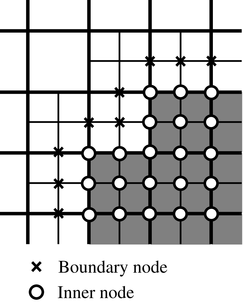
The boundary values of the hierarchical meshes are defined on nodes in buffer cells (Fig. 7). The potential at the boundary is calculated by the coarse-to-fine operator from the lower level following the full weighting scheme. Since the potential on the level $L-1$ meshes reflect the density distribution on the level $L$ meshes after the two grid iteration among them, the potential at the boundary is corrected from the initial guess which is projected from the lower level meshes.

We first wrote a code using the nested iteration which applies the coarse-to-fine projection and the one level red-black Gauss-Seidel iteration instead of the two grid iteration. But a slight discrepancy was observed between the correlation functions in the LCDM model calculated by the nested iteration code with HTS and the code without HTS, though the difference is negligible between the results calculated by the two grid iteration code with and without HTS (§3.4). Hence, it is crucial to adopt the two grid or the multi grid potential solver to implement the HTS technique.

3 Tests of the code

3.1 Force accuracy

As the first test, we have checked whether the force between particles is calculated correctly. First, we placed a truncated singular isothermal sphere. Following the mesh refinement in accordance with the way described in §2.2, the force on the particles is calculated. Then we placed a fiducial particle in a level $L_{D}$ cell randomly and recalculate the force on all particles. Subtracting the previously calculated force from this force, we obtained the gravitational force from the fiducial particle on the rest of particles. We repeated the above process 32 times. In figure 8 the force from the fiducial particle to the rest of particles is plotted against distance between them. Circles, squares, and crosses represent the cases of $L_{D}$= 5, 7, and 9, respectively, while the level of the base mesh is fixed as $L_{B}$=5. In this test, the spacing of the base mesh, the mass of particles, and the gravitational constant are normalized to unity. Although the force is softened when the separation is much smaller than the spacing of the level $L_{D}$ mesh in each case, the force coincides with that expected from the Newtonian law at radius sufficiently larger than this spacing but smaller than the box size.

We also put a homogeneous sphere consists of massless particles added to a massive particle at the center. Setting $N_{\mbox{\small rfn}}=1$ so that all particles belong to the level $L_{D}$ cells, we calculated the force on the massless particles from the central particle. Since our code adopts the periodic boundary condition, we compared this force not with the Newtonian law, but with the sum of the Newtonian force from periodically placed particles which is calculated efficiently using the Ewald expansion (Ewald 1921; Sangster & Dixon 1976). Figure 9 shows the relative error of the force calculated by our code in comparison with that calculated by the Ewald expansion. Circles, squares, and crosses represent the cases of $L_{D}$=6, 8, and 10, respectively, with $L_{B}=6$ in common. In any cases, the error is largest at $r\sim 2l_{L_{D}}$ but is kept within 20%.

3.2 Single plane wave

Zeldovich (1970) formulated the liner approximation for particle trajectories:

$$\mbox{\boldmath{$x$}}=\mbox{\boldmath{$q$}}+b(t)\mbox{\boldmath{$p$}}(\mbox{\boldmath{$q$}}),$$ (30)

where $q$ is the Lagrangian position of the particle and $b(t)$ is the growing mode of the linear density perturbation normalized so that $p$($q$) gives the initial positional perturbation. This Zeldovich approximation is not only applicable to particles in the sub-linear regime, but also gives their exact trajectories for a system of one-dimensional sheets until any pairs of sheets crosses each other. Connecting the trajectories before and after sheet crossings, the trajectories of sheets are calculated with high accuracy. We test our code by comparing the trajectories calculated by our code and those calculated by Yano’s one-dimensional code for which the details are described in Yano & Gouda (1998).

Initially we have imposed a single sinusoidal plane wave perturbation to the Einstein-de Sitter (EdS) universe:

$$p(q) = A\sin(kq),$$ (31)

$$k = \frac{2\pi}{l_{0}},$$ (32)

and

$$A = 10^{-2}l_{L_{B}},$$ (33)

where $l_{0}$ and $l_{L_{B}}$ are the size of simulation box and the base mesh spacing, respectively. In this test, the level of the base mesh is fixed as $L_{B}=5$.

The following equations for position, velocity, and density hold until the first caustic appears:

$$x = q+a(t)A\sin(kq),$$ (34)

$$v = \dot{a}(t)A\sin(kq),$$ (35)

and

$$\rho = \bar{\rho}\left(\frac{\partial x}{\partial q}\right)^{-1}$$ (36)

$$= \bar{\rho}(1+a(t)Ak\cos(kq))^{-1},$$ (37)

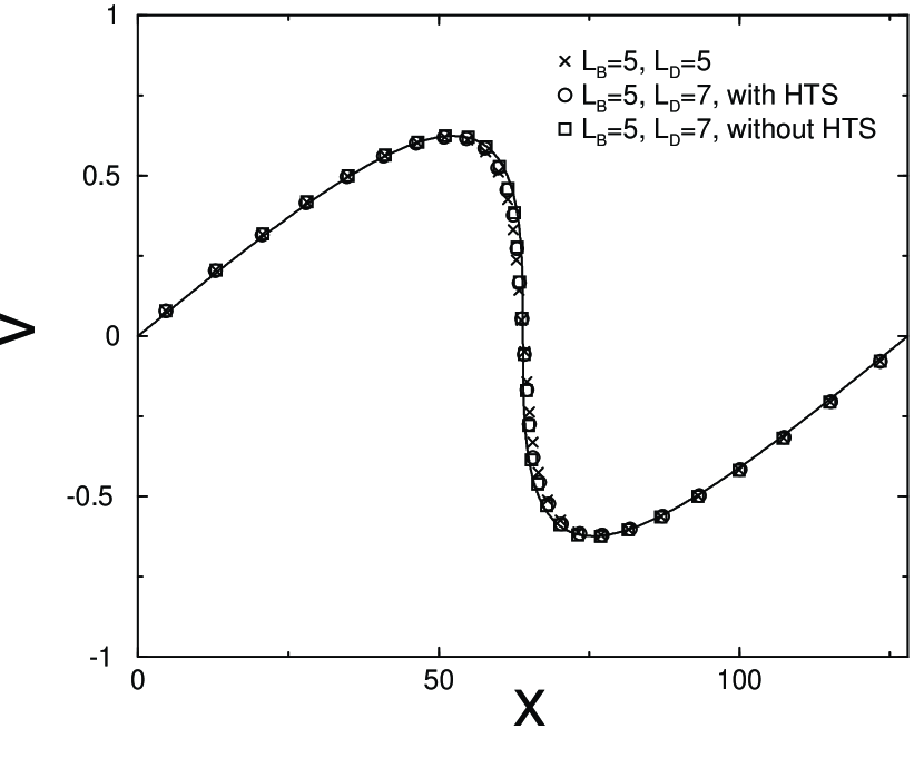
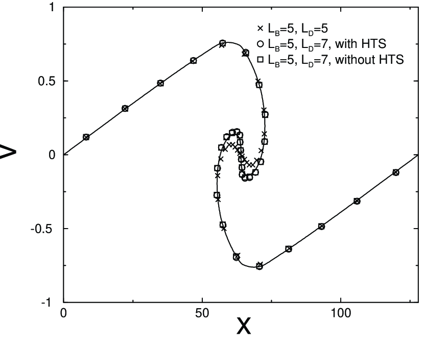
where the scale factor $a(t)$ is normalized to unity at the initial time. When $\rho$ diverges to infinity, the first caustics form. This occurs at $q=\pi k^{-1}=l_{0}/2$ when $a(t)=a_{1}=(Ak)^{-1}$. We run the simulations setting $A=0.01$ with sheets consisting of $L_{B}^{2}=25$ particles arranged on the grid. Figure 10 shows the distribution of sheets in the phase space at $a(t)=a_{1}$ taken from the four runs using the one-dimensional code (solid line), the PM code ($L_{D}=5$, crosses), our code with HTS ($L_{D}=7$, circles), and our code without HTS ($L_{D}=7$, squares). Although the cells bordering on the caustics are refined only once, the velocity degradation for $L_{D}=7$ is weaker than that for $L_{D}=5$.

The difference between the $L_{D}=$5 and 7 results is more prominent when the second caustic appears at $a(t)=a_{2}\simeq 2.34~{}a_{1}$ (Fig. 11). Near the center of the spiral pattern in the phase space, the $L_{D}=5$ result is wound weaker than the other two $L_{D}=7$ results. No obvious difference between the $L_{D}=7$ results with HTS and without it shows that our implementation of the HTS is very successful. 58 base level time steps are used from the beginning of the simulation to the second caustics generation. Note that the positions of the first caustics in the three runs are the same. This is because sheets in low resolution run are pulled toward the center more weakly than those in high resolution runs, not only when they fall toward the center, but also when they leave it in the same way. Thus, the position of caustics does not change much by the resolution of the code. This is the reason why sheets’ position in the phase space is different among low resolution run and high resolution runs, even though the position of the caustics are the same. This is true not only for the plane wave test, but also for the spherical infall test described in the next.

3.3 Spherical self-similar infall

As the third test, our code is checked against the spherical self-similar infall model where the infall of collisionless material onto the collapsed density perturbation in the EdS universe is considered. This model is solved semi-analytically (Fillmore & Goldreich 1984; Bertschinger 1985). As its name indicates, this infall model possesses the symmetry which is different from the planar symmetry of the base mesh in our code and the single plane wave test. Moreover, the infall onto the virialized objects is thought to be common in the hierarchical clustering. For these reasons, this model is widely used as a test for cosmological simulation codes (e.g. Splinter 1996; Kravtsov et al. 1997; Gelato et al. 1997; Yahagi, Mori, & Yoshii 1999).

In order to prepare the initial particle distribution for this test problem, we place $\Delta N$ particles at the center of particles distributed homogeneously and amorphously. Such a distribution is obtained as follows (White, 1993): First, particles are distributed randomly. Next, the system is evolved in the EdS universe reversing the sign of the force to make particles repulsive each other, and is expanded million times from the initial time until the kinetic energy of the system converges to be negligibly small.

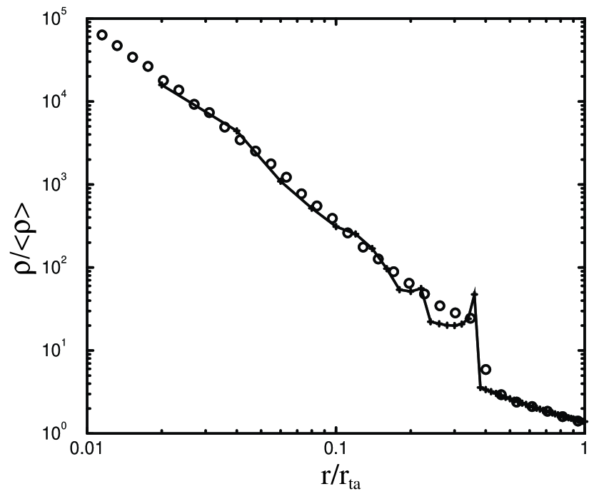
In this test, we set $L_{B}=7$, $L_{D}=10$, $\Delta N=64$, and use $2^{3L_{B}}=128^{3}$ particles. We normalize the time by the initial age of the universe, $\tau=3H_{i}t/2$, and the radius by the turn-around radius, $r_{ta}$, given by

$$r_{ta} = \left(\frac{3\pi}{4}\right)^{-8/9}\delta_{i}^{1/3}R_{i}\tau$$ (38)

$$= \left(\frac{3\pi}{4}\right)^{-8/9}\left(\frac{3}{4\pi}\frac{\Delta N}{N}\right)^{1/3}l_{0}\tau,$$ (39)

where $N$, $\delta_{i}$ and $R_{i}$ are the total number of particles, the initial density contrast and its radial extension, respectively. Figure 12 shows the radial density profile calculated by our code (circles). Crosses connected by the solid line denote the semi-analytic solution taken from Table 4 of Bertschinger (1985). Our result shows good coincidence with the semi-analytic solution including the position of the first caustic and the power law asymptote of density profile toward the center whose index is $-9/4$.

3.4 Halos in the CDM universe

Finally, we have performed three LCDM simulations, using $64^{3}$ particles and $L_{B}=6$ in common. We adopt $L_{D}=6$ for the PM run and $L_{D}=10$ for the AMR+HTS and AMR runs. The difference between the AMR+HTS and AMR runs is only that the AMR+HTS run adopts the HTS while the AMR run does not. For these simulations, we adopt $\Omega_{0}=0.3,\lambda_{0}=0.7,h=0.7$ and $\sigma_{8}=1.0$. The size of simulation box is 70$h^{-1}$ Mpc and the mass of particles is $1.5567\times 10^{11}M_{\odot}$. The initial data of the simulations are generated by the COSMICS code provided by Bertschinger & Bode using the analytic fitting function for the power spectrum of the CDM universe described in Bardeen et al. (1986).

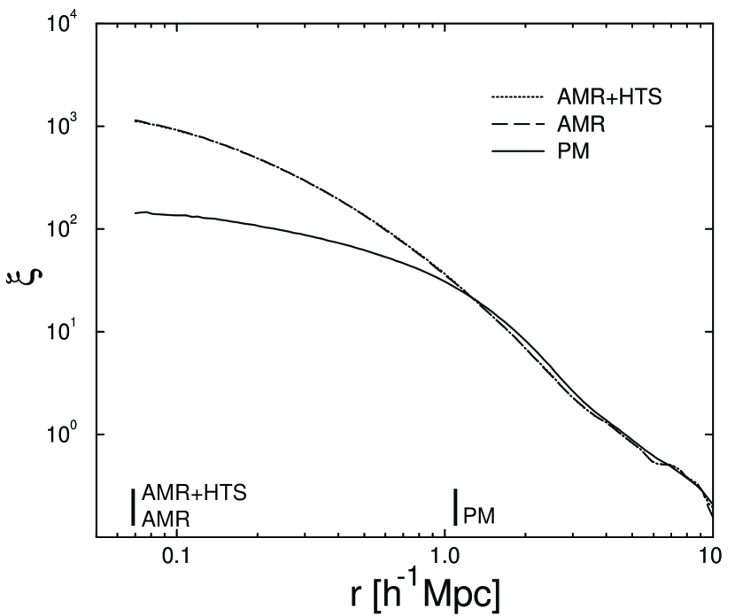
Figure 13 shows the map of projected density in the logarithmic unit at $z=0$. Filtering is not applied to the density maps in any panels. The overall mass distributions from the AMR+HTS and AMR runs agree well with each other, and are more centrally concentrated than that from the PM run. This is confirmed by the comparison among the particle distributions in a slice of 1/16 thickness of the side (Fig. 14), and the two-point correlation functions from the AMR+HTS, AMR, and PM runs (Fig. 15). There are many cosmological $N$-body simulations with parameters similar to our LCDM simulations. Figure 16 shows the correlation function from our AMR+HTS run (thick dotted line) overlaid with those from the PM run in Klypin et al. (1996) (crosses, hereafter KPM run), AP³M run in Jenkins et al. (1998) (dashed line), and ART run in Colín et al. (1999) (solid line). Data of overlaid three runs are taken from figure 4 of Colín et al. (1999). Vertical solid lines shown with $\epsilon_{\mbox{\tiny AMR+HTS}}$, $\epsilon_{\mbox{\tiny PM}}$, $\epsilon_{\mbox{\tiny AP}^{3}\mbox{\tiny M}}$ represent the force resolution of our AMR+HTS run, KPM run, and the AP³M run in Jenkins et al. (1998), respectively. Among the three LCDM simulation runs, the size of the simulation box and the force resolution of the KPM run is closest to those of our AMR+HTS run. The root mean square amplitude of the fluctuation at 8 h^-1Mpc ($\sigma_{8}$) of our run is 1.0 while the KPM run adopted $\sigma_{8}=1.1$. Although the number of particles used in the AMR+HTS run is $1/64$ of particles in the KPM run, magnitude of the correlation function at $r=2\epsilon_{\mbox{\tiny AMR+HTS}}$ of the AMR+HTS run coincides with that of the KPM run within 10$\%$.

We have also compared the density profiles of the halos in the AMR+HTS and AMR runs. Figure 17 shows the density profiles of halos in the AMR+HTS run (circles) and the AMR run (squares). The universal profile proposed by Navarro, Frenk, & White (1996),

$$\rho(r)=\frac{\rho_{s}}{(r/r_{s})(1+r/r_{s})^{2}},$$ (40)

is fitted to the halos in the AMR+HTS run, and the result is denoted by the solid line in each panel of Figure 17. This universal profile provides a good fit to the dark halos over the entire range of radius. The profiles of the halos from the AMR+HTS run are in agreement with those from the AMR run. Slight discrepancies between them are primarily due to the different positions of satellite halos in these two runs. This agreement of halo profiles between the AMR+HTS and AMR runs also indicate that our implementation of the HTS is successful.

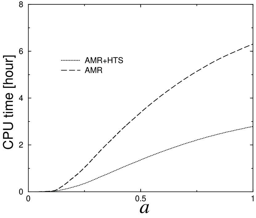
Finally we compare the performance of the AMR+HTS and AMR codes on a PC with an AMD’s Athlon 750 MHz processor. The LCDM simulations for which we set $L_{D}-L_{B}=4$ are performed from $a$=0.0366 to $a$=1. Thereby the AMR+HTS code uses 133 base-level time steps, while the AMR code uses 1932 global time steps. The CPU time spent by these codes is plotted against $a$ in figure 15. As seen from this figure, the AMR+HTS code spends less than a half of the CPU time spent by the AMR code. Thus the AMR+HTS code saves much of the CPU time, while keeping the same spatial resolution as the AMR code. Higher performance of the AMR+HTS code is achieved when we set a higher $L_{D}-L_{B}$.

4 Summary

We have described two techniques of AMR and HTS which are able to increase the spatial and time resolutions of the PM method. The AMR divides and removes cells in each time step in compliance with the refinement criterion, and enhances the spatial resolution. On the other hand, the HTS changes the time step interval depending on the level of particles and enhances the time resolution. Three different tests described in §3 show that our implementation of AMR and HTS is successful. Compared with the previous codes with AMR, we describe the HTS technique in detail. It is found that the HTS is an indispensable technique for the wide dynamic range simulation because importance of the HTS increases as the finer cells are introduced into the simulation.

We will parallelize our code for massively parallel processors to realize simulations with more than $10^{9}$ particles which are needed to study the links between the formation of galaxies and their environments (see. Appendix A). Sorting the hierarchical cells by the Morton ordering is a preparatory step for the parallelization.

Finally it is worth mentioning that we have already combined our $N$-body code with the hydrodynamics code (Yahagi & Yoshii, 2000). This combined code enables us to study the dynamical evolution of both dark matter and baryonic components. Including some physical and phenomenological processes such as cooling of the gas, star formation, energy feedback from supernovae etc, we will trace the formation process of galaxies under the realistic condition in the universe.

Appendix A Crude estimation for the number of particles required to resolve halos of field galaxies

The relaxation time scale for a halo is given by (see e.g. Binney & Tremaine 1987)

$$t_{relax} \sim \frac{0.1N}{\ln N}t_{cross}$$ (A1)

$$\sim \frac{0.1N}{\ln N}(G\rho)^{-1/2},$$ (A2)

where $N$ is the number of particles which compose the halo. For a halo formed at $z=z_{coll}$ in the Einstein-de Sitter (EdS) universe, we have

$$t_{relax} \sim \frac{0.1N}{\ln N}(178~{}G\rho_{0}(1+z_{coll})^{3})^{-1/2}.$$ (A3)

In order to calculate the evolution of the halo correctly, the relaxation time scale must exceed the age of the halo at $z=0$, i.e.

$$t_{relax} \gtrsim t_{age}$$ (A4)

$$\gtrsim \frac{2}{3}H_{0}^{-1}(1-(1+z_{coll})^{3/2}).$$ (A5)

The required minimum number of particles, $N_{relax}$, can be estimated crudely by solving the following non-linear equality:

$$t_{relax}(N_{relax})=t_{age}.$$ (A6)

Thus the total number of particles, required to keep simulated galactic halos unrelaxed, is given by

$$N_{total} \geq \frac{M_{total}}{M_{halo}}N_{relax}$$ (A7)

$$\simeq 2.78~{}\left(\frac{M_{halo}}{10^{11}M_{\odot}}\right)^{-1}\left(\frac{L}{1\mbox{Mpc}}\right)^{3}\Omega_{0}h^{2}N_{relax}$$ (A8)

$$\sim 10^{9},~{}~{}(L\sim 32\mbox{Mpc},~{}z_{coll}\sim 3,~{}\mbox{EdS})$$ (A9)

where $M_{halo}$ is the minimum mass of halos which do not relax until the simulation is completed, and $L$ is the size of simulated region. For the reference values of $M_{halo}=10^{11}M_{\odot},L=32\mbox{Mpc},z_{coll}=3$, and $(\Omega_{0},h)=(1,0.5)$, we have $N_{total}\gtrsim 10^{9}$ for the EdS universe.

The above estimate is based on many assumptions. For example, halos are assumed to have been isolated after they formed, although there are cluster galaxies which interact with the cluster and other galaxies, and these interactions can increase the required number of particles. Hence, this estimation is quite naive and optimistic, but it gives the lower limit of the number of particles necessary to reproduce un-relaxed galactic haloes in simulations.

Appendix B Pseudo-code

$base\_step$ ()
{
             int L;
             
             $time\_steps$();
             $velocity\_half\_step$(L${}_{\mbox{\tt B}}\leq$L$\leq$L${}_{\mbox{\tt D}}$);
             if (L${}_{\mbox{\tt B}}<$ L${}_{\mbox{\tt D}}$) $hierarchical\_step$(L${}_{\mbox{\tt B}}+1$);
             $position\_step$(L${}_{\mbox{\tt B}}\leq$L$\leq$L${}_{\mbox{\tt D}}$);
             $mesh\_modification$(L${}_{\mbox{\tt B}}+1\leq$L$\leq$L${}_{\mbox{\tt D}}$);
             $potential\_solver$(L${}_{\mbox{\tt B}}\leq$L$\leq$L${}_{\mbox{\tt D}}$);
             $velocity\_half\_step$(L${}_{\mbox{\tt B}}\leq$L$\leq$L${}_{\mbox{\tt D}}$);
}

$hierarchical\_step$ (int L₀)
{
             int L;
             
             if (L${}_{0}<$ L${}_{\mbox{\tt D}}$) $hierarchical\_step$(L${}_{0}+1$);
             $position\_step$(L${}_{0}\leq$L$\leq$L${}_{\mbox{\tt D}}$);
             $mesh\_modification$(L${}_{0}+1\leq$L$\leq$L${}_{\mbox{\tt D}}$);
             $potential\_solver$(L${}_{0}\leq$L$\leq$L${}_{\mbox{\tt D}}$);
             $velocity\_full\_step$(L${}_{0}\leq$L$\leq$L${}_{\mbox{\tt D}}$);
             if (L${}_{0}<$ L${}_{\mbox{\tt D}}$) $hierarchical\_step$(L${}_{0}+1$);
}

Appendix C Coarse-to-fine and fine-to-coarse operators

The full-weighting scheme for the fine-to-coarse and the coarse-to-fine operators are adopted as

$$A^{L-1}_{l,m,n}= \frac{1}{8} A^{L}_{2l,2m,2n}+$$

$$\frac{1}{16} (A^{L}_{2l-1,2m,2n}+A^{L}_{2l+1,2m,2n}+A^{L}_{2l,2m-1,2n}+A^{L}_{2l,2m+1,2n}+A^{L}_{2l,2m,2n-1}+A^{L}_{2l,2m,2n+1})+$$

$$\frac{1}{32} (A^{L}_{2l-1,2m-1,2n}+A^{L}_{2l+1,2m-1,2n}+A^{L}_{2l-1,2m+1,2n}+A^{L}_{2l+1,2m+1,2n}+$$

$$A^{L}_{2l-1,2m,2n-1}+A^{L}_{2l+1,2m,2n-1}+A^{L}_{2l-1,2m,2n+1}+A^{L}_{2l+1,2m,2n+1}+$$

$$A^{L}_{2l,2m-1,2n-1}+A^{L}_{2l,2m+1,2n-1}+A^{L}_{2l,2m-1,2n+1}+A^{L}_{2l,2m+1,2n+1})+$$

$$\frac{1}{64} (A^{L}_{2l-1,2m-1,2n-1}+A^{L}_{2l+1,2m-1,2n-1}+A^{L}_{2l-1,2m+1,2n-1}+A^{L}_{2l+1,2m+1,2n-1}+$$

$$A^{L}_{2l-1,2m-1,2n+1}+A^{L}_{2l+1,2m-1,2n+1}+A^{L}_{2l-1,2m+1,2n+1}+A^{L}_{2l+1,2m+1,2n+1}),$$

$$A^{L+1}_{2l,2m,2n}= A^{L}_{l,m,n},$$

$$A^{L+1}_{2l+1,2m,2n}= \frac{1}{2} (A^{L}_{l,m,n}+A^{L}_{l+1,m,n}),$$

$$A^{L+1}_{2l,2m+1,2n}= \frac{1}{2} (A^{L}_{l,m,n}+A^{L}_{l,m+1,n}),$$

$$A^{L+1}_{2l,2m,2n+1}= \frac{1}{2} (A^{L}_{l,m,n}+A^{L}_{l,m,n+1}),$$

$$A^{L+1}_{2l+1,2m+1,2n}= \frac{1}{4} (A^{L}_{l,m,n}+A^{L}_{l+1,m,n}+A^{L}_{l,m+1,n}+A^{L}_{l+1,m+1,n}),$$

$$A^{L+1}_{2l+1,2m,2n+1}= \frac{1}{4} (A^{L}_{l,m,n}+A^{L}_{l+1,m,n}+A^{L}_{l,m,n+1}+A^{L}_{l+1,m,n+1}),$$

$$A^{L+1}_{2l,2m+1,2n+1}= \frac{1}{4} (A^{L}_{l,m,n}+A^{L}_{l,m+1,n}+A^{L}_{l,m,n+1}+A^{L}_{l,m+1,n+1}),$$

and

$$A^{L+1}_{2l+1,2m+1,2n+1}= \frac{1}{8} (A^{L}_{l,m,n}+A^{L}_{l+1,m,n}+A^{L}_{l,m+1,n}+A^{L}_{l,m,n+1}+$$

$$A^{L}_{l+1,m+1,n}+A^{L}_{l+1,m,n+1}+A^{L}_{l,m+1,n+1}+A^{L}_{l+1,m+1,n+1}).$$

Here, $A^{L}_{i,j,k}$ represents any variables defined on the node which is placed at $(x,y,z)=(i~{}l_{L},j~{}l_{L},k~{}l_{L})$ on the level $L$ mesh.

Figure 1: Data structure of the building block which is used to construct the hierarchical meshes. Eight half-sized cells having the same parent are grouped into a cell octet and share the pointer to the parent and its six neighbors.

Figure 2: Construction of the hierarchical meshes by connecting cell octets as shown. These cell octets are added or removed dynamically as the system evolves. The cells without the child cell octet use their pointer to the child octet as the pointer to the head of the linked listed particles which reside in the cell.

Figure 3: Three types of the hierarchical meshes such as unrefined, refined and buffer cells. All cells which satisfy the refinement criterion are subdivided and called refined cells (shaded). Those cells which are next to the refined cells are also subdivided and called buffer cells. The others remain as unrefined cells.

Figure 4: An example of the hierarchical mesh distribution in the $N$-body code with AMR for the case of the LCDM universe described in §3.4. When particles are distributed as shown in the left panel, hierarchical meshes are placed as shown in the right panel. The shape of the hierarchical meshes is not geometrically restricted.

Figure 5: Schematic illustration of the full multigrid method. The full multigrid method accelerates the relaxation process by reducing the long wavelength mode of the residual using the coarser meshes. The full multigrid iteration begins from the coarsest mesh, i.e., the whole simulation box. Potential on the level $L_{0}$ mesh is solved using level $L$ meshes where $0\leq L\leq L_{0}$.

Figure 6: Schedule of the Poisson solver in our AMR code for the case of $L_{B}=2$ and $L_{D}=4$. At time $t$, we execute the full multigrid iteration first. Then we apply the two grid iteration from $L_{B}+1$ to $L_{D}$. When the level $L$ particles step their position, the two grid iteration is applied from $L-1$ to $L_{D}$.

Figure 7: Location of inner nodes (circles) and outer nodes (crosses) on which the potential and the boundary condition are defined respectively. The inner nodes are placed on the corners of refined cells, and the outer nodes in buffer cells.

Figure 8: Pairwise force in the AMR code. Circles, squares, and crosses are for $L_{D}=$5, 7, 9, respectively, with $L_{B}=5$ in common. The size of the base mesh, the mass of particle, and the gravitational constant are normalized to unity. The solid line shows the exact Newtonian force of $g=r^{-2}$. The vertical lines at the bottom indicate the size of the smallest cell for three cases.

Figure 9: Error of the pairwise force calculated by the AMR code. Circles, squares, and crosses are for $L_{D}=$6, 8, 10, respectively, with $L_{B}=6$ in common. Error is defined as the relative error of the calculated force using the AMR code in comparison with that calculated by the Ewald expansion. In all cases, the error is maximized at $r\sim 2l_{L_{D}}$, but is kept within 20%.

Figure 10: Snapshot of the phase diagram from the single plane wave test at the epoch of first caustic generation. The solid line shows the exact solution calculated by the one-dimensional code with 1024 sheets using the code described in Yano & Gouda (1998). Crosses, circles, and squares show the results obtained by the code without AMR, with AMR and HTS, and with AMR but without HTS, respectively. Because the meshes are refined only once at this epoch, the difference between the AMR and non-AMR results is minor. We however note that this difference becomes larger as time proceeds beyond the first caustic generation (see Fig. 11).

Figure 11: Snapshot of the phase diagram from the single plane wave test at the epoch of second caustic generation. The same as figure 10, but for $a_{2}\simeq 2.34~{}a_{1}$ where $a_{1}$ and $a_{2}$ are the scale factors at the epoch of first and second caustics generation, respectively. Although blunt in the non-AMR run, the second caustics are well captured in the AMR result, irrespective of whether the HTS is included or not.

Figure 12: Density profile of the spherical self-similar infall model. Crosses connected by the solid line show the semi-analytic solution provided in Table 4 of Bertschinger (1985). The circles show the result by our code, where radius and density are normalized by the turn around radius and the mean density, respectively. Our result shows good agreement with the semi-analytic solution including the first caustic.

Figure 13: Map of projected density in the logarithmic unit at $z=0$ for the LCDM universe with $\Omega_{0}=0.3,\lambda_{0}=0.7,h=0.7$ and $\sigma_{8}=1.0$. The size of simulation box is 70$h^{-1}$ Mpc, and the number of particles is $64^{3}$ and the level of the base mesh, $L_{B}$, $=6$. Three panels are taken from (a) AMR run with $L_{D}=10$, (b) AMR+HTS run with $L_{D}=10$, and (c) PM run with $L_{D}=L_{B}=6$. The overall mass distributions of (a) and (b) agree well with each other, and their halos are bound more tightly than those in (c).

Figure 14: The same as figure 13. Distributions of particles in the LCDM simulation are shown in this figure. Only particles in a slice of 1/16 thickness of the simulation box side are shown. This figure confirms the trends described in the caption of figure 13.

Figure 15: Two-point correlation function at $z=0$ for the LCDM universe with $\Omega_{0}=0.3,\lambda_{0}=0.7,h=0.7$ and $\sigma_{8}=1.0$, based on the same simulations as in figure 13. Shown are the results from the AMR+HTS run (solid line), the AMR run (dotted line), and the PM run (broken line). Note that the AMR+HTS and AMR runs give almost identical results, so that the difference is not visible in this figure. The vertical lines indicate the minimum size of the cell, or the force resolution of the codes. Because of the low spatial resolution the correlation function at small separations in the result of the PM run is strongly weakened compared with the other two runs.

Figure 16: Comparison of the correlation function of LCDM simulations. Shown are our AMR+HTS run (thick dotted line), the PM run in Klypin et al. (1996) (crosses), the AP³M run in Jenkins et al. (1998) (dashed line), and the ART run in Colín et al. (1999) (solid line). Vertical solid lines shown with $\epsilon_{\mbox{\tiny AMR+HTS}}$, $\epsilon_{\mbox{\tiny PM}}$, $\epsilon_{\mbox{\tiny AP}^{3}\mbox{\tiny M}}$ represent the force resolution of our AMR+HTS run, KPM run, and the AP³M run in Jenkins et al. (1998), respectively.

Figure 17: Density profiles of halos detected at $z=0$ for the LCDM universe with $\Omega_{0}=0.3,\lambda_{0}=0.7,h=0.7$ and $\sigma_{8}=1.0$, based on the same simulations as in figure 13. Shown are the results from the AMR+HTS (circles) and AMR (squares) runs. The solid lines show the fits to the halos in the result of the AMR+HTS run using the universal density profile (Eq. 40).

Figure 18: CPU time spent by the AMR+HTS run (dotted line) and the AMR run (dashed line) on a PC with an AMD’s Athlon 750Hz processor. The AMR+HTS run spends only a half of the CPU time spent by the AMR run.

References

- Aarseth (1963) Aarseth, S. J. 1963, MNRAS, 126, 223
- Anninos et al. (1994) Anninos, P., Norman, M. L., & Clarke, D. A. 1994, ApJ, 436, 11
- Bardeen et al. (1986) Bardeen, J. M., Bond, J. R., Kaiser, N., & Szalay, A. S. 1986, ApJ, 304, 15
- Barnes & Hut (1989) Barnes, J. E., & Hut, P. 1989, ApJS, 70, 389
- Berger & Oliger (1984) Berger, M. J., & Oliger, J. 1984 J. Comp. Phys., 53, 484
- Bertschinger (1985) Bertschinger, ApJS, 58, 39
- Binney & Tremaine (1987) Binney, J., & Tremaine, S. 1987, Galactic Dynamics (Princeton University Press: Princeton)
- Brandt (1977) Brandt, A. 1977, Mathematics of Computation, 31, 333
- Briggs (1987) Briggs, W. L. 1987, A Multigrid Tutorial (Society of Industrial and Applied Mathematics: Philadelphia)
- Colín et al. (1999) Colín, P., Klypin, A. A., Kravtsov, A. V., & Khokhlov A. M. 1999, ApJ, 523, 32
- Ewald (1921) Ewald, P. P. 1921, Ann. Phys., 64, 253
- Fillmore & Goldreich (1984) Fillmore, J. A., & Goldreich, P. 1984, ApJ, 281, 1
- Gelato et al. (1997) Gelato, S., Chernoff, D. F., & Wasserman, I. 1997, ApJ, 480, 115
- Hockney & Eastwood (1988) Hockney, R. W., & Eastwood, J. W. 1988, Computer simulation using particles (Institute of Physics Publishing: Bristol)
- Jankins et al. (1998) Jenkins, A., Frenk, C. S., Pearce, F. R., Thomas, P. A., Coleberg, J. M., White, S. D. M., Couchman, H. M. P., Peacock, J. A., Efstathiou, G., & Nelson, A. H. 1998, ApJ, 499, 20
- Jessop et al. (1994) Jessop, C., Duncan, M., & Chau, W. Y. 1994, J. Comp. Phys., 115, 339
- Khokhlov (1998) Khokhlov, A. M. 1998, J. Comp. Phys., 143, 519
- Klypin et al. (1996) Klypin, A. A., Primack, J., & Holtzman, J. 1996, ApJ, 466, 13
- Kravtsov et al. (1997) Kravtsov, A. V., Klypin, A. A., & Khokhlov, A. M. 1997, ApJS, 111, 73
- Kravtsov et al. (1998) Kravtsov, A. V., Klypin, A. A., Bullock, J. S., & Primack, J. 1998, ApJ, 502, 48
- Makino (1991) Makino, J. 1991, PASJ, 1991, 43, 859
- Navarro et al. (1996) Navarro, J. F., Frenk, C. S., & White S. D. M. 1996, ApJ, 462, 563
- Norman & Bryan (1999) Norman, M. L. & Bryan, G. L. 1999, in Numerical Astrophysics, ed. S. Miyama, K. Tomisaka & T. Hanawa (Dordrecht: Kluwer), 19
- Press et al. (1992) Press, W. H., Teukolsky, S. A., Vetterling, W. T., & Flannery, B. P. 1992, Numerical Recipes 2nd ed. (Cambridge University Press: Cambridge)
- Sangster & Dixon (1976) Sangster, M. I. L., & Dixon, M. 1976, Adv. Phys., 25, 247
- Splinter (1996) Splinter R. J. 1996, MNRAS, 281, 281
- Suisalu & Saar (1995) Suisalu, I., & Saar, E. 1995, MNRAS, 274, 287
- Villumsen (1989) Villumsen, J. V. 1989, ApJS, 71, 407
- Warren & Salmon (1993) Warren, M. S., & Salmon, J. K., 1993, in Supercomputing ’93 (Los Alamitos: IEEE Computer society), 12
- White (1993) White, S. D. M. 1993, in Cosmology and Large Scale Structure, Les Houches Session LX, ed. R. Schaeffer, J. Silk, M. Spiro, & J. Zimn-Justin (Amsterdam: Elsevier), 349
- Yahagi et al. (1999) Yahagi, H., Mori, M., & Yoshii, Y. 1999, ApJS, 124, 1
- Yahagi & Yoshii (2000) Yahagi, H., & Yoshii, Y. 2000, in ASP Conf. Ser., Physics of Galaxy Formation, ed. M. Umemura, & H. Susa (San Francisco: ASP)
- Yano & Gouda (1998) Yano, T., & Gouda, N. 1998, ApJS, 118, 274
- Zeldovich (1970) Zeldovich, Ya. B. 1970, A&A, 5, 84