The Fundamental Plane of Spiral Galaxies: Theoretical Expectations

Abstract

Current theory of disk galaxy formation is used to study fundamental-plane (FP) type of relations for disk galaxies. We examine how the changes in model parameters affect these relations and explore the possibility of using such relations to constrain theoretical models. The distribution of galaxy disks in the space of their fundamental properties are predicted to be concentrated in a plane, with the Tully-Fisher (TF) relation (a relation between luminosity $L$ and maximum rotation velocity $V_{m}$) being an almost edge-on view. Using rotation velocities at larger radii generally leads to larger TF scatter. In searching for a third parameter, we find that both the disk scale-length $R_{d}$ (or surface brightness) and the rotation-curve shape are correlated with the TF scatter. The FP relation in the $(\,{\rm Log}\,L,\,{\rm Log}\,V_{m},\,{\rm Log}\,R_{d})$-space obtained from the theory is $L\propto R_{d}^{\alpha^{\prime}}V_{m}^{\beta^{\prime}}$, with ${\alpha^{\prime}}\sim 0.50$ and ${\beta^{\prime}}\sim 2.60$, consistent with the preliminary result we obtain from observational data. Among the model parameters we probe, variation in any of them can generate significant scatter in the TF relation, but the effects of the spin parameter and halo concentration can be reduced significantly by introducing $R_{d}$ while the scatter caused by varying $m_{d}$ (the ratio between disk mass and halo mass) is most effectively reduced by introducing the parameters which describes the rotation-curve shape. The TF and FP relations combined should therefore provide useful constraints on models of galaxy formation.

1 Introduction

Spiral galaxies are characterized by their flattened disks (with approximately exponential profiles) and nearly flat rotation curves. The main observational parameters that describe the overall properties of a spiral galaxy are the central surface brightness $\mu_{0}$, the disk scale-length $R_{d}$ and the characteristic rotation velocity (e.g. the maximum rotation velocity $V_{m}$). The observed disk population covers a large range in these parameters, with $\mu_{0}$ varying from $\sim 24$ (low surface brightness galaxies) to $\sim 20\,\rm{mag\,arcsec^{-2}}$, $R_{d}$ from $\sim 0.1$ to $\sim 10\,{\rm{kpc}}$, and $V_{m}$ from $\sim 50$ to $\sim 300\,{\rm{km\,s^{-1}}}$. Despite the diversities, spiral galaxies obey a well-defined scaling relation between their total luminosity $L$ and maximum rotation velocity $V_{m}$. This relation (called the Tully-Fisher relation, hereafter TF relation) is usually expressed in the form

$$L=AV_{m}^{\beta^{\prime}}\,,$$ (1)

where $\beta^{\prime}$ is the slope, and $A$ is the zero-point. The observed TF relation is quite tight. For example, in the $I$-band, the scatter in luminosities for a fixed $V_{m}$ is only about 0.38 magnitude (Giovanelli et al. 1997). Thus, the TF relation can be used as a relative distance indicator for spiral galaxies. It is still unclear whether the scatter in the observed TF relation is dominated by observational errors or by intrinsic variations. Since intrinsic scatter must exist to some degree, a natural question is whether there is a third parameter that correlates with the residual scatter of the TF relation. The situation is quite similar to that for elliptical galaxies. Although elliptical galaxies are found to obey the Faber-Jackson relation (a relation between luminosity $L$ and central velocity dispersion $\sigma$), the fundamental-plane (hereafter FP) relation (with the introduction of a third parameter, the effective radius $r_{e}$) has much smaller scatter (Djorgovski & Davis 1987; Dressler et al. 1987). For disk galaxies, due to the broad distribution of scale-length $R_{d}$, one obvious choice of the third parameter is $R_{d}$ or the central surface brightness $\mu_{0}$ ($\mu_{0}$ and $R_{d}$ are related by $L=2\pi\mu_{0}R_{d}^{2}$ for an exponential disk). On the other hand, since disk galaxies also present diversities in their rotation-curve shapes (Persic, Salucci & Stel 1996), another possible choice may be a parameter that characterizes the rotation-curve profile.

Much effort has been made in searching for this third parameter (e.g. Kodaira 1989; Han 1991; Tully & Verheijen 1997; Willick et al. 1997; Courteau & Rix 1999; Willick 1999), but the results are still inconclusive. While most of the studies cited above concluded that the third parameter is not crucial, some of them did find evidence for the existence of a third parameter (e.g. Kodaira 1989; Willick 1999). More recently, Koda, Sofue & Wada (2000a) obtained a scaling plane in the form of $L\propto(VR)^{\beta^{\prime}}$ from both observational data and numerical simulations. But the radius $R$ in this relation is not really a new degree of freedom, because it is bounded to the rotation velocity $V$ with the same power index $\beta^{\prime}$.

From theoretical side, there are many attempts to understand the formation of disk galaxies in the framework provided by current cosmogonic models (e.g. CDM models: Fall & Efstathiou 1980; White & Frenk 1991; Dalcanton, Spergel & Summes 1997; Mo, Mao & White 1998, hereafter MMW). The current standard scenario of disk formation assumes that galaxy disks form as a result of gas cooling in dark matter haloes. Detailed modeling shows that such models are quite successful in interpreting observational data, especially the observed TF relation (MMW; van den Bosch 1998, 2000; Avila-Reese, Firmani & Hernandez 1998; Weil, Eke & Efstathiou 1998; Heavens & Jimenez 1999; Mo & Mao 2000; Navarro & Steinmetz 2000; Koda, Sofue & Wada 2000b; Zou & Han 2000; Cole et al. 2000; Buchalter, Jimenez & Kamionkowski 2001). In the CDM cosmogonies, the characteristic rotation velocity of a disk galaxy is determined largely by the potential of the dark matter while the luminosity of the disk is given by the amount of stars (baryons) in the disk. The observed TF relation therefore implies a tight relation between the disk mass and the depth of the dark halo potential well, and its scatter may be used to constrain models of galaxy formation.

Our main goal in this paper is to examine whether FP-like relations exist for the disk population based on current theoretical models of disk formation, and to provide some theoretical guidelines for the search of FP-like relations. Moreover, we explore the possibility of using such relations as a tool to understand galaxy formation by examining the response of the theoretical scaling relations to the changes of model parameters.

The structure of the paper is as follows. Section 2 presents the model and summarizes the model parameters. In Section 3, we search for the theoretical FP relation and examine its responses to the variations of model parameters. In Section 4, some preliminary results obtained from observational data are presented and compared with our model predictions. Finally, in Section 5, we make further discussions and summarize our main conclusions.

2 Theoretical model

2.1 Disk Formation

Our model here follows that presented in Mo, Mao & White (1998, hereafter MMW). We refer the reader to that paper for details; here we only introduce the main ingredients relevant to our analyses.

The initial density profiles of dark haloes are assumed to take the universal form,

$$\rho(r)=\frac{\rho_{crit}\delta_{0}}{(r/r_{s})(1+r/r_{s})^{2}}\,,$$ (2)

where $r_{s}$ is a characteristic radius, $\rho_{crit}$ is the critical density and $\delta_{0}$ is a constant (Navarro, Frenk & White 1997, hereafter NFW). We define the radius of a dark halo to be $r_{200}$ within which the mean density is 200 times the critical density, and represent the characteristic radius by the concentration, $c\equiv r_{200}/r_{s}$. It is then easy to show that

$$\delta_{0}={200\over 3}{c^{3}\over\ln(1+c)-c/(1+c)}\,.$$ (3)

The radius $r_{200}$ and mass $M$ of a halo can be expressed in terms of its circular velocity $V_{c}$ as

$$r_{200}=\frac{V_{c}}{10H(z)}\,,~{}M=\frac{{V_{c}}^{2}r_{200}}{G}\,,$$ (4)

where $G$ is the gravitational constant, and $H(z)$ is the Hubble constant at redshift $z$. We relate the initial angular momentum $J$ of a halo to its spin parameter $\lambda$ through the definition

$$\lambda=J|E|^{1/2}G^{-1}M^{-5/2},$$ (5)

where $E$ is the total energy of the halo. A dark halo is therefore described by three parameters: the circular velocity $V_{c}$, the concentration $c$ and the spin parameter $\lambda$. As a result of dissipative and radiative processes, the gas component gradually settles into a disk. We assume the disk mass to be a fraction $m_{d}$ of the halo mass, and the disk angular momentum to be $j_{d}$ times $J$. Thus, two other parameters, $j_{d}$ and $m_{d}$ are introduced to relate the halo properties to the properties of the final disk. Following MMW, we also assume that disks have exponential surface density profiles with a constant mass-to-light ratio $\Upsilon$, and that dark haloes respond to disk growth adiabatically. Under these assumptions, we can obtain the luminosity $L$, the disk scale length $R_{d}$ and the rotation curve $V(R)$ for a given set of model parameters. Specifically,

$$L=\frac{m_{d}M}{\Upsilon}\,,~{}R_{d}=\frac{1}{\sqrt{2}}\left(\frac{j_{d}}{m_{d}}\right)\lambda{r_{200}}f_{r}\,,~{}V(R)=V_{c}f_{v}(R)\,,$$ (6)

where $f_{r}$ and $f_{v}$ are factors which depend on halo profile and disk action. We use the same procedure outlined in MMW to calculate $f_{r}$ and $f_{v}$ as functions of $c$, $j_{d}$, $m_{d}$ and $\lambda$.

2.2 Model Parameters

As discussed above, five parameters ($V_{c}$, $\lambda$, $c$, $m_{d}$ and $j_{d}$) need to be specified for individual haloes in order to predict the properties of the disks that form within them. In this subsection we describe one by one how these parameters are chosen in our modelling.

2.2.1 Halo circular velocity $V_{c}$

The distribution of halo masses is derived from the Press-Schechter formalism (Press & Schechter 1974, hereafter PS) applied to the $\Lambda$CDM cosmogony (with mass density parameter $\Omega_{0}=0.3$, cosmological constant $\Omega_{\Lambda}=0.7$, Hubble’s constant $h=0.7$, perturbation-spectrum normalization $\sigma_{8}=1$). We select the host haloes of disks with circular velocities in the range from $50\,{\rm{km\,s^{-1}}}$ to 300$\,{\rm{km\,s^{-1}}}$ at redshift $z=0$. The choice of cosmogony does not change our main results, because we are not interested in the exact distribution of galaxies with respect to mass.

2.2.2 Halo spin parameter $\lambda$

N-body simulations show that the distribution of halo spin parameter $\lambda$ can be approximated by a log-normal function,

$$p(\lambda)\,d\lambda=\frac{1}{\sqrt{2\pi}\sigma_{\ln\lambda}}\exp\left[-\frac{\ln^{2}(\lambda/\bar{\lambda})}{2\sigma_{\ln\lambda}^{2}}\right]\frac{d\lambda}{\lambda},$$ (7)

with $\bar{\lambda}$=0.05 and $\sigma_{\ln\lambda}=0.5$. This distribution is found to be quite independent of cosmology and of halo mass (Warren et al. 1992; Lemson & Kauffmann 1999). Syer, Mao & Mo (1999) obtained a similar distribution function for $\lambda$ from the observational data of disk sizes. In this paper, we use equation (7) for the distribution of $\lambda$.

2.2.3 Halo concentration $c$

The halo concentration, $c$, may depend on halo formation history and cosmogony. Simulations show that the circular-velocity dependence of the NFW concentration $c$ can be approximated by

$$c_{\rm NFW}\approx c_{\rm NFW*}(V_{c}/100\,{\rm{km\,s^{-1}}})^{-1/3}$$ (8)

(see NFW). Using $N$-body simulations, Jing (2000) found that the distribution of $c$ for the majority of his simulated haloes can be described by a log-normal function with a mean $\bar{c}$ slightly smaller than that of the NFW result:

$$p(c^{\prime})dc^{\prime}=\frac{1}{\sqrt{2\pi}\sigma_{\ln c^{\prime}}}\left[-\frac{\ln^{2}(c^{\prime}/\bar{c}^{\prime})}{2\sigma_{\ln c^{\prime}}^{2}}\right]d\ln c^{\prime}\,,~{}c^{\prime}\equiv c/c_{\rm NFW}\,,$$ (9)

where $\bar{c}^{\prime}=0.85$ and $\sigma_{\ln c^{\prime}}=0.25$. In this paper, we take $c_{\rm NFW*}=10$ as is given in the original NFW paper, use equation (8) to obtain $c_{\rm NFW}$ and equation (9) for the distribution of $c$.

2.2.4 The mass ratio $m_{d}$

This parameter represents the ratio between the disk mass and the total halo mass. The processes by which gas cools into a disk to form stars are complicated and not well understood at the present time. Nevertheless, some limits can be set. First, the value of $m_{d}$ should be smaller than the overall baryon fraction in the universe $\Omega_{B}/\Omega_{0}$, which is about 0.1 for a low-density universe with $\Omega_{0}=0.3$ and $h=0.7$, and about 0.05 for an Einstein-de Sitter universe with $h=0.5$, according to the cosmic nucleosynthesis theory. Second, the value of $m_{d}$ should not be much smaller than 0.01, because disks with lower gas content may not be able to form sufficient amount of stars to be included in a TF sample. Thus, we set the range of $m_{d}$ to be from 0.01 to 0.1 and take 0.05 as the typical value. We will also consider a case where $m_{d}$ changes systematically with $V_{c}$.

2.2.5 The angular-momentum ratio $j_{d}$

This parameter characterizes the ratio between the specific angular momentum of the disk and that of the dark halo. Although disk material may have the same initial specific angular momentum as the dark matter, little is known about the transfer of angular momentum between gas and dark matter in subsequent evolutions. From earlier theoretical considerations (e.g. MMW) we know that $j_{d}\approx m_{d}$ is required in order to ensure the predicted disk sizes to match observations. In our model, we allow $j_{d}$ to have $50\%$ chance to be in the range $0.5m_{d}$–$1m_{d}$, and another $50\%$ chance to be in the range $1m_{d}$–$2m_{d}$. Thus, we adopt for $j_{d}$ a simple distribution function of the form:

$$p(j_{d})dj_{d}=\left\{\begin{array}[]{ll}dj_{d}/m_{d}&\mbox{for $0.5\,m_{d}\leq j_{d}<m_{d}$}\\ dj_{d}/(2m_{d})&\mbox{for $m_{d}\leq j_{d}<2\,m_{d}$}\end{array}\right.\,.$$ (10)

2.3 Monte-Carlo Realization

In order to search for a FP relation for theoretical disks, we need to choose three observable parameters to define the plane. We take the luminosity $L$ and a characteristic rotation velocity $V$ as the two fundamental quantities. In most of our discussions, we use the maximum velocity $V_{m}$ as the characteristic velocity, but we also discuss the effects of using rotation velocities at other radii. For the third quantity, we try two different choices based on the discussion in the previous section: the disk scale-length $R_{d}$ and a rotation-curve shape parameter $\Gamma$ (to be defined below).

The procedure for obtaining the FP is as follows. We first generate a Monte-Carlo sample of 1000 haloes from the PS formalism, with $V_{c}$ in the range between 50 and $300\,{\rm{km\,s^{-1}}}$. We then assign to each halo the other four parameters by Monte-Carlo simulations. Finally we use the model of MMW to predict the properties of each model galaxy. As in MMW, we exclude unstable disks with

$$\epsilon_{m}\equiv\frac{V_{m}}{{(GM_{d}/R_{d})}^{1/2}}<0.9\,,$$ (11)

where $M_{d}=m_{d}M$ is the gas mass of the disk (e.g. Christodoulou, Shlosman & Tohline 1995). On the other hand, galaxies with very low density may not form stars. We therefore also exclude disks with Toomre parameter

$$Q\equiv\frac{\sigma\kappa}{\pi G\Sigma}>1.4\,,$$ (12)

where $\sigma$ is the gas velocity dispersion, $\kappa$ is the epicyclic frequency, and $\Sigma$ is the mass surface density (Kennicutt 1989). In our model, we use the average surface mass density inside the half-mass radius (about $1.68R_{d}$) to replace $\Sigma$, and adopt $\sigma=6\,{\rm{km\,s^{-1}}}$. We assume that all disks have the same mass-to-light ratio and take $\Upsilon\approx 1.7h$ in the $I$-band (Bottema 1997). All the results are for disks at $z=0$ and we take $h=0.7$ whenever an explicit value of $h$ is used.

3 Model Predictions

3.1 Results Based on Maximum Rotation Velocity and Disk Scale-length

In this section, we try to find the FP of disk galaxies in the $(\,{\rm Log}\,L$-$\,{\rm Log}\,V_{m}$-$\,{\rm Log}\,R_{d})$-space. The reason is clear: while $L$ and $V_{m}$ are the two parameters in the conventional TF relation, the choice of $R_{d}$ as the third parameter is motivated by the fact that disk galaxies cover a large range of $R_{d}$. We define the FP as

$$M_{I}=\alpha\,\,{\rm Log}\,R_{d}({\,{\rm{kpc}}})+\beta\,\,{\rm Log}\,V_{m}({\,{\rm{km\,s^{-1}}}})+\gamma,$$ (13)

where $M_{I}$ is the absolute magnitude of the disk in the $I$-band, $\alpha$, $\beta$ and $\gamma$ are constants which are obtained by a least-square fit of equation (13) to the Monte-Carlo data. In the disk model outlined above, there are four parameters, $\lambda$, $m_{d}$, $j_{d}$ and $c$, whose effects on the FP relation need to be evaluated. If all these four parameters are set to be constant, the predicted TF relation is a line with no scatter. The scatter in any one of these four parameters can cause scatter in the TF relation (see e.g. MMW, Mo & Mao 2000). The first question is whether some of the scatter can be eliminated or reduced in the FP relation. In order to show this, we first construct four samples where scatter is allowed only in one of the four model parameters while the other parameters taking their typical values (see Table 1). In these cases, we ignore the selection criteria given by equations (11) and (12), and so some of the model galaxies in these samples may not correspond to any realistic disks. The scaling relations are shown in Figure 1, while the fitting results of these relations are listed in Table 1. The scatters on both the TF relation and the FP relation are represented by the root-mean-square deviation ($rms$) of $M_{I}$.

Figure 1: The effects of changing individual model parameters (as indicated in the panels) on the TF and FP relations. (a), (b), (c) and (d) show the effects of $\lambda$, $j_{d}$, $c$ and $m_{d}$ respectively. In each case, the left panel shows the FP relation (the magnitude $M_{I}$ as a function of $\alpha\,{\rm Log}\,R_{d}+\beta\,{\rm Log}\,V_{m}+\gamma$, where the values of $\alpha$, $\beta$ and $\gamma$ are listed in Table 1), whereas the right panel shows the corresponding TF relation (the solid line being the linear regression). The scatter in $M_{I}$ is represented by the $rms$ deviation.

Comparing the scatter of the TF relation and the corresponding FP relation, we see that the introduction of $R_{d}$ as the third parameter is very effective in reducing the scatter caused by $\lambda$, $j_{d}$ and $c$ but less so in reducing the scatter caused by $m_{d}$. Notice that the FPs in different cases are tilted significantly with each other, except cases of varying $\lambda$ and $j_{d}$ (see Table 1).

Table 1: The effects of changing individual model parameters on the TF relation and the FP relation defined by equation (13). Column 1 lists the name of each case, columns 2 to 6 give the model parameters (which are either a single number, or a range, or an equation of distribution), columns 7 to 9 show the fitting results for the FP relation, while columns 10 and 11 list the scatter of the magnitude $M_{I}$ in the FP and TF relations, respectively

Case	$\lambda$	$j_{d}$	$c$	$m_{d}$	$\Upsilon$	$\alpha$	$\beta$	$\gamma$	$\sigma_{\rm FP}$	$\sigma_{\rm TF}$
$\lambda$	eq. (7)	0.05	8.5	0.05	$1.7h$	$-1.29$	$-6.16$	$-7.21$	0.08	0.39
$j_{d}$	0.05	eq. (10)	0.05	8.5	$1.7h$	$-1.21$	$-6.27$	$-7.05$	0.04	0.29
$c$	0.05	0.05	eq. (9)	0.05	$1.7h$	$-2.89$	$-4.61$	$-9.83$	0.002	0.23
$m_{d}$	0.05	$m_{d}$	8.5	0.01–0.1	$1.7h$	1.11	$-8.53$	$-3.23$	0.12	0.20

After an preview of the effects of individual model parameters on the scaling relations, we now examine cases where scatter is allowed in more than one model parameters. For clarity, we list all cases in Table 2. In all these cases, the selection criteria given by equations (11) and (12) are imposed.

Table 2: The predicted TF ($M_{I}$-$\,{\rm Log}\,V_{m}$) and FP ($M_{I}$-$\,{\rm Log}\,V_{m}$-$\,{\rm Log}\,R_{d}$) relations in various cases (Case VI will be discussed in Subsection 3.4). The table structure is the same as Table 1.

Case	$\lambda$	$j_{d}$	$c$	$m_{d}$	$\Upsilon$	$\alpha$	$\beta$	$\gamma$	$\sigma_{\rm FP}$	$\sigma_{\rm TF}$
I	eq. (7)	eq. (10)	8.5	0.05	$1.7h$	$-0.95$	$-6.54$	$-6.64$	0.03	0.21
II	eq. (7)	eq. (10)	eq. (9)	0.05	$1.7h$	$-1.22$	$-6.43$	$-6.65$	0.15	0.35
III	eq. (7)	eq. (10)	8.5	0.01–0.1	$1.7h$	$-1.27$	$-6.35$	$-6.79$	0.32	0.44
IV	eq. (7)	eq. (10)	eq. (9)	0.01–0.1	$1.7h$	$-1.48$	$-6.35$	$-6.61$	0.34	0.50
V	eq. (7)	eq. (10)	eq. (9)	0.01–0.1	eq. (15)	$-0.79$	$-6.47$	$-6.85$	0.33	0.38
VI	eq. (7)	eq. (10)	eq. (9)	eq. (18)	$1.7h$	$-1.09$	$-8.11$	$-2.90$	0.22	0.35

3.1.1 Effects of $\lambda$ and $j_{d}$

Since the TF relation is, for a constant disk mass-to-light ratio, a relation between the disk mass and the maximum rotation velocity, difference in the disk angular momenta may cause scatter in the TF relation because, for a given disk mass, the contribution by the disk to the rotation velocity depends on disk angular momentum. The disk specific angular momentum is characterized by the product $\lambda j_{d}$ and so we examine the effects of these two parameters together. We generate a Monte-Carlo sample, with $\lambda$ and $j_{d}$ following the distributions described in equations (7) and (10), while keeping $m_{d}=0.05$ and $c=8.5$ (see Case I in Table 2).

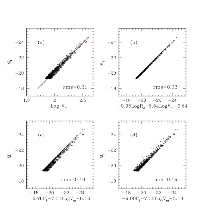
Figure 2: The predicted TF and FP relations for Case I in Table 2. The predicted TF relation is shown in panel (a) together with the fit to the model prediction (solid line) and the fit to the observational result of Dale et al. (1999b) (dashed line). Panel (b) shows the FP with $R_{d}$ as the third parameter, while panel (c) and (d) show the FPs based on the two different rotation-curve shape parameters $\Gamma_{1}$ and $\Gamma_{2}$ (to be discussed in Subsection 3.3).

Panel (b) of Figure 2 shows the FP, while the corresponding TF relation is shown in panel (a) together with a comparison to the observational result of Dale et al. (1999b). We see that there is an almost perfect FP in this case, although there is significant TF scatter caused by the variations of the spin parameter $\lambda$ and angular-momentum ratio $j_{d}$. The observed slope and zero-point of the TF relation are well reproduced, which is consistent with the result already found in MMW. The FP is given by $\alpha=-0.95$, $\beta=-6.54$, with a zero-point $\gamma=-6.64$. The FP scatter in $M_{I}$ is only 0.03 mag, much smaller than the predicted TF scatter ($0.21\,$mag). Thus, the scatter in the TF relation caused by $\lambda j_{d}$ can be eliminated almost entirely by the third parameter $R_{d}$. So, if the scatter in the TF relation were caused entirely by the dispersion in the spin, the model would predict a perfect FP for the disk population. However, the predicted TF scatter ($0.21\,$mag ) is lower than the observed value of Dale et al. ($0.38\,$mag, see also Giovanelli et al. 1997), implying that other factors are also important in causing the observed TF scatter.

3.1.2 Effect of $c$

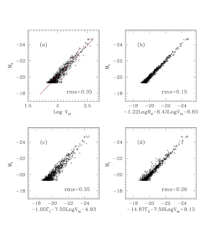
Figure 3: The predicted FP and TF relations for Case II in Table 2. The setting of the panels is the same as in Figure 2.

Here we include the scatter caused by the distribution of $c$, in addition to those by $\lambda$ and $j_{d}$, but still keep $m_{d}=0.05$. The results are shown in Figure 3. In this case (Case II in Table 2), the observed TF relation is also well reproduced. The predicted FP (with $\alpha=-1.22$, $\beta=-6.43$ and $\gamma=-6.65$) is close to Case I shown in Figure 1, except the scatter is larger ($0.15\,$mag). This scatter in the FP is still substantially smaller than that in the predicted TF relation ($0.35\,$mag). The introduction of $R_{d}$ cannot eliminate all the scatter, because the FP defined by $c$ is tilted with respect to that defined by $\lambda$ and $j_{d}$ (see Table 1).

3.1.3 Effect of $m_{d}$

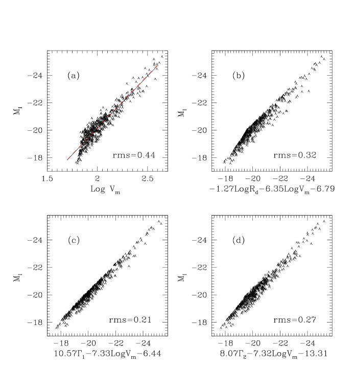
Figure 4: The predicted FP and TF relations for Case III in Table 2. The setting of the panels is the same as in Figure 2.

To examine the effect of $m_{d}$ on the scaling relations, we construct a Monte-Carlo sample with a fixed concentration ($c=8.5$), with $\lambda$ and $j_{d}$ having their typical distributions, and with $m_{d}$ randomly drawn from 0.01 to 0.1 (Case III in Table 2). As discussed in Subsection 2.2.4, this range of $m_{d}$ covers the values expected from any reasonable considerations. We keep $c$ constant, in order to single out the effect of $m_{d}$. The results are shown in Figure 4. In this case, the slope and zero-point of the FP ($\alpha=-1.27$, $\beta=-6.35$ and $\gamma=-6.79$) are comparable to those shown in Figures 2 and 3. The scatter in the predicted TF relation ($0.44\,$mag) is much larger than those in Case I and II and even larger than that in the observations of Giovanelli et al. (1997). This large predicted scatter is obviously a consequence of the large range of $m_{d}$ used in this case. The scatter in the FP relation ($0.32\,$mag) is also quite large, suggesting that the scatter produced by the variation of $m_{d}$ has a large tilt with respect to that caused by $\lambda$ and $j_{d}$ (see Table 1).

3.1.4 A general case

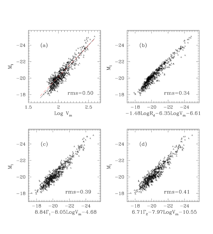
Figure 5: The predicted FP and TF relations for Case IV in Table 2. The setting of the panels is the same as in Figure 2.

As a summary, we consider a case where scatter is allowed in all of the model parameters (Case IV in Table 2). The results are shown in Figure 5. Although generous amount of scatter is assumed for each of the model parameters, a FP can still be defined for the model galaxies, with $\alpha=-1.48$, $\beta=-6.35$ and $\gamma=-6.61$. The predicted TF relation has a scatter ($0.50\,$mag) larger than that observed, again mainly due to the large range of $m_{d}$ assumed. The scatter of the FP is also quite large ($0.34\,$mag). This is not surprising, because the scatter is dominated by the variation in $m_{d}$.

If we express the FP in the form $L\propto R_{d}^{\alpha^{\prime}}V_{m}^{\beta^{\prime}}$, the slopes $\alpha^{\prime}$ and $\beta^{\prime}$ change only little for different cases, and the FP relation for the model disks can be represented by

$$L\propto R_{d}^{\alpha^{\prime}}V_{m}^{\beta^{\prime}}\,,~{}\mbox{with}~{}\alpha^{\prime}=0.49\pm 0.10\,,~{}\beta^{\prime}=2.60\pm 0.05\,,$$ (14)

where the errors represent the scatter among different cases. Thus, the luminosity of a disk galaxy is mainly determined by $V_{m}$, and so the TF relation is almost an edge-on view of the FP. However, the residual dependence on $R_{d}$ is also significant, due to the fact that the range of $R_{d}$ for the observed disks is quite large.

3.1.5 A case with varying $\Upsilon$

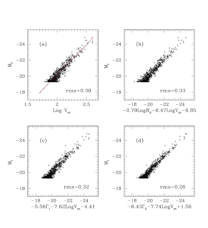
Figure 6: The predicted FP and TF relations for Case V in Table 1. The setting of the panels is the same as in Figure 2.

Although we did not include the disk mass-to-light ratio $\Upsilon$ in the list of our model parameters above, it obviously is another parameter in the model. In order to compare model predictions directly with observations, we need to convert the predicted disk mass to a disk luminosity, which requires an assumption about the disk mass-to-light ratio. Scatter in the disk mass-to-light ratio therefore also gives rise to scatter in both the TF and the FP relation. Clearly, the induced scatter is along the $M_{I}$ axis, with a $rms$ (in terms of the luminosity) exactly the same as that in the mass-to-light ratio.

The exact value of $\Upsilon$ for a galaxy depends on its star formation history and is in general difficult to model accurately. As an example, we consider a case (Case V in Table 2) where the disk mass-to-light ratio is assumed to be

$$\Upsilon=1.7h(m_{d}/0.05)$$ (15)

and all other parameters are assumed to be the same as in Case IV. In this case, the effect of $m_{d}$ on the magnitude $M_{I}$ is eliminated, and so the TF scatter caused by $m_{d}$ is only through its effect on the rotation curve. The results are shown in Figure 6. The predicted TF relation has scatter smaller than that in Case IV because the effect of $m_{d}$ on $M_{I}$ is eliminated [see Equation (6)]. The scatter of the predicted FP ($0.33\,$mag) is close to that of the predicted TF relation ($0.38\,$mag), implying that the scatter in the TF relation caused by $m_{d}$ through disk action cannot be effectively reduced by introducing $R_{d}$ as the third parameter.

From the results presented above we can conclude that variations in the mass ratio $m_{d}$ and in the mass-to-light ratio may be important sources of scatter in the predicted TF and FP relations. If the variations in $m_{d}$ and $\Upsilon$ are small, the scatter in the predicted FP relation may be significantly lower than that in the TF relation. On the other hand, if the scatter in the observed TF relation is mainly due to the variations in $m_{d}$ and $\Upsilon$, the introduction of the third parameter $R_{d}$ will not reduce the scatter significantly. Thus, by comparing the scatter in the TF relation with the scatter in the FP relation, one may hope to find the main sources of scatter in the two scaling relations. We will come back to this issue in Section 4.

3.2 Results Based on Rotation Velocities at Other Radii

Although the maximum rotation velocity ($V_{m}$) is commonly used in defining the TF relation (mainly for observational reasons, because the inclination-corrected 21 cm line width of a disk galaxy is assumed to be twice its maximum rotation velocity), there is no a priori reason against using rotation velocities at other radii. Such definition is possible for disk galaxies with measured rotation curves. Since the disk contribution to the rotation curve may change with radius (for example, the rotation curve of a galaxy at large radius is expected to be dominated by dark matter while the disk contribution may be significant in the inner region), analyses of the TF relation (or the FP relation) using rotation velocities at different radii may provide more information on the mass components of disk galaxies.

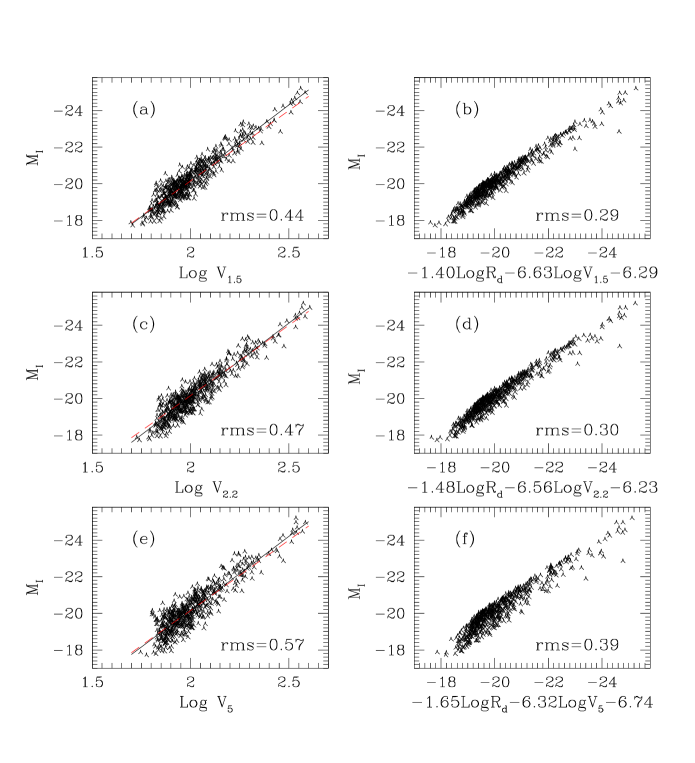
Figure 7: The predicted TF and FP relations based on different rotation velocities. The right panels show the FPs with $R_{d}$ as the third parameter, using respectively $V_{1.5}$, $V_{2.2}$ and $V_{5}$ (all in units of $\,{\rm{km\,s^{-1}}}$) as the characteristic rotation velocity. The left panels show the corresponding TF relations. The solid lines in the TF panels are the fits to the model predictions, while the dashed lines represent the relation observed by Dale et al. (1999b).

Observationally, there are some attempts to define the TF relation using rotation velocities other than the maximum rotation velocity, in the hope of getting smaller scatter. For example, Courteau (1997) found an optimal TF relation using rotation velocities at $2.2R_{d}$, while there are also claims that the TF relation is optimized if rotation velocities at smaller radii are used (see Willick 1999 and references therein). Interestingly, almost all of these analyses showed that the scatter in the TF relation becomes larger when the amplitudes of the rotation curves at large radii are used.

In this section, we use our theoretical model to examine the effect of using different rotation velocities on the TF and FP relations. Specifically, we choose three representative radii, $R=5R_{d},2.2R_{d},1.5R_{d}$, to define the characteristic rotation velocities ($V_{5}$, $V_{2.2}$ and $V_{1.5}$). For most of our model rotation curves, the maximum rotation velocity is reached at $R\sim 3R_{d}$ (MMW), and so $V_{5}$ represents the rotation velocity well beyond the peak of a rotation curve. $V_{2.2}$ is chosen because the rotation velocity of a pure exponential disk peaks at $R\approx 2.16R_{d}$, while $V_{1.5}$ is chosen to represent the inner part of the rotation curve.

We construct a Monte-Carlo sample in the same way as described in Subsection 2.3. The distributions of all the model parameters are assumed to be the same as the general case (Case IV) in Table 2. The results are shown in Figure 7 and summarized in Table 3.

Table 3: The same as Table 2 except that other rotation velocities are used instead of $V_{m}$.

Case	$\lambda$	$j_{d}$	$c$	$m_{d}$	$\Upsilon$	$\alpha$	$\beta$	$\gamma$	$\sigma_{\rm FP}$	$\sigma_{\rm TF}$
$V_{1.5}$	eq. (7)	eq. (10)	eq. (9)	0.01-0.1	$1.7h$	$-1.40$	$-6.63$	$-6.29$	0.29	0.44
$V_{2.2}$	eq. (7)	eq. (10)	eq. (9)	0.01-0.1	$1.7h$	$-1.48$	$-6.56$	$-6.23$	0.30	0.47
$V_{5}$	eq. (7)	eq. (10)	eq. (9)	0.01-0.1	$1.7h$	$-1.65$	$-6.32$	$-6.74$	0.39	0.57

As shown in Figure 7, the model predictions are consistent with the observations that the use of rotation velocities at larger radii generally leads to larger scatters in the TF relations. This result can be understood as follows. At very large radii, the disk contribution to the rotation curve is negligible, and so the variation in $m_{d}$ does not affect the rotation velocities very much. Since the luminosity of a disk is directly proportional to $m_{d}$ (for a constant mass-to-light ratio), the variation in $m_{d}$ affects the TF scatter directly. This effect is reduced in the cases where rotation velocities in the inner part (e.g. $V_{2.2}$ and $V_{1.5}$) are used, because of the increasing halo-disk interaction (Mo & Mao 2000; Navarro & Steinmetz 2000). We have also made calculations for models where $m_{d}$ is kept constant. In such cases, the TF scatter is almost independent of the definition of the characteristic rotation velocity. Thus, the scatter in the TF relations defined at different rotation velocities may be used to constrain the variation of the mass ratio $m_{d}$.

Similar to the TF relations, the scatter in the FP relation is also larger when the rotation velocities at larger radii are used. This is because $R_{d}$ cannot effectively reduce the TF scatter caused by $m_{d}$.

3.3 Rotation-Curve Shape as the Third Parameter

Since rotation curves of individual galaxies have different shapes, it is possible that the TF scatter is correlated with the rotation-curve shape. Persic & Salucci (1990) considered this possibility from observational data. In the theoretical model we are considering here, the shapes of rotation curves can be affected by all the four model parameters, and so the TF scatter must be correlated to the rotation-curve shape to some degree. In this subsection, we carry out a quantitative analysis of such correlation. To do this, we use two parameters similar to those defined by Persic, Salucci & Stel (1996),

$$\Gamma_{1}=\left(\frac{d\,\,{\rm Log}\,\,V}{d\,\,{\rm Log}\,\,R}\right)_{2.2R_{d}},~{}~{}~{}\Gamma_{2}=\frac{V_{5}}{V_{2.2}},$$ (16)

to represent the rotation-curve shapes in the inner and outer regions. We investigate the FP in the space spanned by $M_{I}$, $\,{\rm Log}\,(V_{m})$ and $\Gamma_{1}$ ($\Gamma_{2}$) for all the cases considered above. The simulated FP is fitted to the relation

$$M_{I}=\alpha\Gamma+\beta\,{\rm Log}\,V_{m}(\,{\rm{km\,s^{-1}}})+\gamma,$$ (17)

where $\Gamma$ is either $\Gamma_{1}$ or $\Gamma_{2}$. The predicted FPs are shown in panel (c) and panel (d) in each of Figures 2–6, and the fitting results are summarized in Table 4.

Table 4: The predicted FP relations where the rotation-curve shape parameters $\Gamma_{1}$ and $\Gamma_{2}$ are adopted as the third parameter. Column 1 lists the name of each case as listed in Table 2. Columns 2 to 5 give the fit results for the FP in the $M_{I}$-$\,{\rm Log}\,V_{m}$-$\Gamma_{1}$ space, while columns 6 to 9 are those for the FP in the $M_{I}$-$\,{\rm Log}\,V_{m}$-$\Gamma_{2}$ space.

		$\Gamma_{1}$					$\Gamma_{2}$
Case	$\alpha$	$\beta$	$\gamma$	$\sigma_{\rm FP}$		$\alpha$	$\beta$	$\gamma$	$\sigma_{\rm FP}$
I	6.76	$-7.31$	$-6.16$	0.19		$-9.00$	$-7.38$	3.19	0.19
II	$-1.05$	$-7.55$	$-4.93$	0.35		$-14.87$	$-7.05$	9.13	0.26
III	10.57	$-7.33$	$-6.44$	0.21		8.07	$-7.32$	$-13.31$	0.27
IV	8.84	$-8.05$	$-4.68$	0.39		6.71	$-7.97$	$-10.55$	0.41
V	$-5.56$	$-7.62$	$-4.41$	0.32		$-6.43$	$-7.74$	1.56	0.26
VI	$-0.28$	$-9.97$	$0.44$	0.35		$-8.57$	$-10.69$	1.94	0.34

These results show that the introduction of the shape parameter of rotation curves as the third parameter can reduce the scatter of the TF relation, but the two parameters considered here are less effective than $R_{d}$ in all the cases except in Case III where the TF scatter is effectively reduced by the introduction of $\Gamma_{1}$ or $\Gamma_{2}$. This suggests that these shape parameters are effective in reducing the scatter caused by $m_{d}$ (due to disk action) but not so much in reducing the scatter caused by $\lambda$$j_{d}$ and $c$.

Unfortunately, $\Gamma_{1}$ and $\Gamma_{2}$ are both more difficult to measure than $R_{d}$ from observations, and it is not yet possible to obtain such a FP from observational data. Notice that the slope $\alpha$ associated with the two shape parameters is very sensitive to the change of model parameters, because the ranges of these parameters are relatively small.

Figure 8: The edge-on view of the FP in the space spanned by $M_{I}$, $\,{\rm Log}\,R_{d}$, $\,{\rm Log}\,V_{m}$, $\Gamma$ (or $\Gamma_{2}$) for Case IV. Notice that the scatter in $M_{I}$ is reduced significantly relative to that shown in Figure 5.

From the above discussion we see that the disk scale-length $R_{d}$ is effective in reducing the TF scatter caused by $\lambda j_{d}$ (Figure 2) and $c$ (Figure 3), while the rotation-curve shape parameters are more effective in reducing the scatter caused by $m_{d}$ (Figure 4). It is therefore interesting to see what happens if both $R_{d}$ and one of the rotation-curve shape parameters are introduced to define a plane in the four-dimensional space spanned by $M_{I}$, $\,{\rm Log}\,R_{d}$, $\,{\rm Log}\,V_{m}$, and $\Gamma_{1}$ (or $\Gamma_{2}$). The results are shown in Figure 8 for Case IV. As expected, the scatter is significantly reduced.

3.4 A case where $m_{d}$ changes with $V_{c}$

In reality, the value of $m_{d}$ may depend systematically on halo circular velocity, as is the case if feedback effects can eject gas more effectively from smaller haloes (e.g. White & Frenk 1991). To model this effect, we construct a sample where $m_{d}$ is assumed to change with $V_{c}$ as

$$m_{d}=0.1\left[1+\left(\frac{150\,{\rm{km\,s^{-1}}}}{V_{c}}\right)^{2}\right]^{-1}(1+\delta)\,,$$ (18)

where $\delta$ is a random number between $-0.1$ and 0.1. Other parameters are chosen the same as in Case IV. This case is listed as Case VI in Tables 2 and 4, and the results are shown in Figure 9.

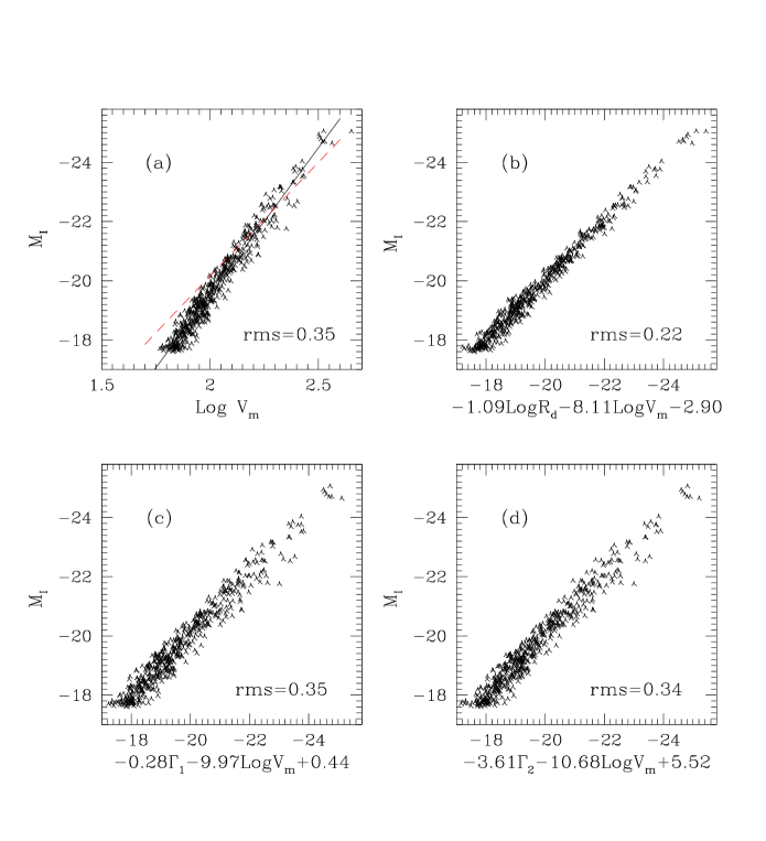
Figure 9: The predicted FP and TF relations for Case VI in Table 2. The setting of the panels is the same as Figure 2

In this case the TF relation is $M_{I}=-9.75\,{\rm Log}\,V_{m}-0.03$ [the solid line in panel (a) of Figure 9], which has a much steeper slope ($\beta\approx 3.8$) than all other cases we have considered. Correspondingly, the slope $\beta$ in the FP relation (with $R_{d}$ as the third parameter) is also steeper, but the value of $\alpha$ does not change much (see Table 2). The introduction of $\Gamma_{1}$ (or $\Gamma_{2}$) as the third parameter does not help much in reducing the TF scatter because, with the assumed small scatter in $m_{d}$, the TF scatter is dominated by the variations in $\lambda$$j_{d}$ and $c$.

Figure 10: The correlation between $M_{I}$ and the rotation-curve shape parameters, $\Gamma_{1}$ and $\Gamma_{2}$. The top two panels are for Case IV while the lower two panes are for Case VI where $m_{d}$ is correlated with $V_{c}$ as in Equation (18).

Since the rotation-curve shape parameters are correlated with $m_{d}$, it is interesting to see if these parameters can be used to reveal the trend of $m_{d}$ with $V_{c}$. To do this, we examine the correlation between $M_{I}$ and $\Gamma_{1}$ (or $\Gamma_{2}$) for Case VI and compare the results with those for Case IV. The results are shown in Figure 10. As one can see, if $m_{d}$ is correlated with $V_{c}$, then there is a strong correlation between $M_{I}$ and $\Gamma_{1}$ (or $\Gamma_{2}$), in the sense that more luminous galaxies have smaller $\Gamma_{1}$ (or $\Gamma_{2}$). Such correlations are in fact observed by Persic, Salucci & Stel (1996), but the data are still too uncertain to give any meaningful constraints on the model.

4 Comparison with Preliminary Observational Results

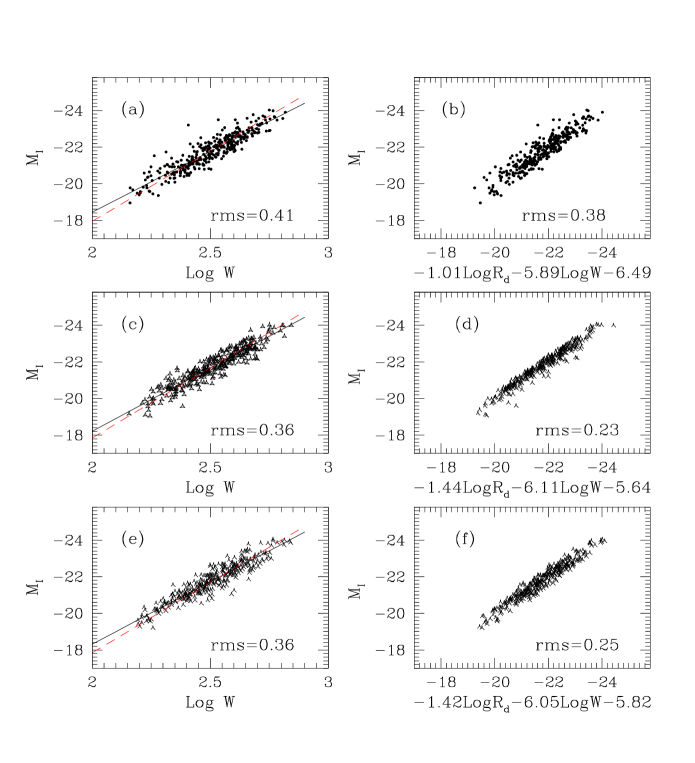
Figure 11: The observed and simulated FP and TF relations based on the data from Dale et al.(1999a). Panel (a) shows the FP while panel (b) shows the TF relation. Panels (c), (d), (e) and (f) show the FPs and TF relations for two simulated samples which have the same distributions in $L$ and $R_{d}$ as the observed sample. Panels (c) and (d) show the theoretical predictions of Case IV. Panels (e) and (f) show the theoretical predictions of a sample with the same parameter as Case II except that the mass-to-light ratio $\Upsilon$ is assumed to be random between $1h$ and $2h$. The solid lines in three TF panels are the direct fit to the data point, while the dashed lines show the result obtained by Dale et al. (1999b) after bias correction.

Having seen the theoretical expectations for the scaling relations of spiral galaxies, one is obviously interested in seeing what observations actually show. Here we present some preliminary results without going into the details of the observational selection effects, leaving a more sophisticated analysis to a future paper.

The data we use are from Dale et al. (1999a), which presents TF observations for 35 rich Abell clusters of galaxies in the $I$-band, along with the exponential scale-lengths $R_{d}$. We simply use the published data without correcting for any bias. Panel (a) and (b) of Figure 11 show the results. The FP for the observed galaxies can be described as

$$M_{I}=-1.01\,{\rm Log}\,R_{d}(\,{\rm{kpc}})-5.89\,{\rm Log}\,W(\,{\rm{km\,s^{-1}}})-6.49,$$ (19)

where $W$ is the velocity width, which we assume to be twice $V_{m}$. The index on $R_{d}$ is comparable to that given by the models presented above, but the index on $W$ (or $V_{m}$) is lower than the model predictions. This lower value is almost certainly due to observational bias. In order to show this, we construct a sample with the same model parameters as in the general case (Case IV) and select model galaxies with the same luminosity and size distributions as the observed sample so as to reproduce the selection effect. The results are shown in panels (c) and (d) of Figure 11. As one can see, the TF and FP slopes for this sample are quite close to the observed values. Note that the scatter is smaller than that of Case IV in Figure 5, indicating the selection effect is important. As another example, we show in panels (e) and (f) the results for a sample with the same model parameters as in Case II except that $\Upsilon$ has a random distribution between $1h$ and $2h$ and with galaxies also selected according to the observed luminosity and size distributions. We see that the scatter allowed in $\Upsilon$ (a factor of two) is much smaller than that in $m_{d}$ (a factor of ten), again because disk action reduces TF scatter (Mo & Mao 2000). In both cases, the scatter in the FP is significantly smaller than that observed. Unfortunately, it is unclear how seriously these discrepancies should be taken. The bias correction required may be more complicated than what is assumed here. In particular, the observed sample is for cluster galaxies, and so systematic bias may also arise from some environmental effects which are not modelled in the theory.

5 Discussion and Summary

In this paper, we use current theory of disk galaxy formation to study whether a FP-like relation is expected for spiral galaxies. After examining in detail how the changes in model parameters affect the scaling relations of disk galaxies, we find that the fundamental properties of disk galaxies are generally concentrated into a plane, with the TF relation representing an almost edge-on view. We made a systematical search for the third parameter which may correlate with the TF scatter. We find that the disk scale-length $R_{d}$ (or surface brightness) as the third parameter can effectively reduce the scatter of TF relation, especially that caused by the variations of halo spin and concentration. The rotation-curve shape as the third parameter can be used to reduce the scatter caused by $m_{d}$. For the various cases we analyzed, the FPs in the $(\,{\rm Log}\,L,\,{\rm Log}\,V_{m},\,{\rm Log}\,R_{d})$-space are quite similar and well represented by equation (14). This relation is consistent with the preliminary results we obtain from observational data.

We also discuss the possibility of using other characteristic velocities [e.g. $V_{5}$, $V_{2.2}$ and $V_{1.5}$] instead of $V_{m}$ as the velocity parameter in the TF and FP relations. The theory is consistent with the observations that the scatter in the TF relation is generally larger when rotation velocities at larger radii are used.

There are, however, a number of uncertainties in the theoretical model, which must be taken into account when comparing models with observations. Real galaxies may be much more complicated than our simple model implies: galaxy disks may not be perfectly exponential, the mass distribution in dark haloes may be non-spherical and clumpy and so the rotation curves may not be smooth, and the existence of galactic bulges may affect both the rotation curve and the luminosity profile. Furthermore, the assumption of a constant disk mass-to-light ratio (in the $I$-band), although consistent with current observations, is clearly unrealistic, because the mass-to-light ratio of a galaxy depends on its star formation history. None of these issues are easy to resolve, but we hope the present paper can provide some theoretical guidelines for the search of scaling relations for disk galaxies.

References

- [1] Avila-Reese V., Firmani C., Hernarndez X., 1998, ApJ, 505, 37
- [2] Cole S., Lacey C.G., Baugh C.M., Frenk C.S., 2000, MNRAS, 319, 168
- [3] Bottema R., 1997, A&A, 328, 517
- [4] Buchalter A., Jimenez R., Kamionkowski M., 2001, MNRAS, 322, 43
- [5] Chritodoulou D.M., Shlosman I., Tohline J.E., 1995, ApJ, 443, 551
- [6] Courteau S., 1997, AJ, 114, 2402
- [7] Courteau S., Rix H.W., 1999, ApJ, 513, 561
- [8] Dalcanton J.J., Spergel D.N., Summers F.J., 1997, ApJ, 482, 659
- [9] Dale D.A., Giovanelli R. Haynes M.A., Campusano L.E., Hardy E., 1999a, AJ, 118, 1468
- [10] Dale D.A., Giovanelli R. Haynes M.A., Campusano L.E., Hardy E., 1999b, AJ, 118, 1489
- [11] de Jong R., Lacey C., 2000, ApJ, 545, 781
- [12] Djorgovski S., Davis M., 1987, ApJ, 313, 59
- [13] Dressler A., Lynden-Bell D., Burstein D., Davies R.L., Faber S.M., Terlevich R.J., Wegner G., 1987, ApJ, 313, 42
- [14] Fall S.M., Efstathiou G., 1980, MNRAS, 193, 189
- [15] Giovanelli R., Haynes M.P., Herter T., Vogt N.P., da Cost L.N., Freudling W., Salzer J.J., Wegner G., 1997, AJ, 113, 53
- [16] Han M., 1992, ApJS, 81, 35
- [17] Heavens A.F., Jimenez R., 1999, MNRAS, 305, 770
- [18] Jing Y.P., 2000, ApJ, 535, 30
- [19] Kennicutt R.C., Jr., 1989, ApJ, 498, 541
- [20] Koda J., Sofue Y., Wada K., 2000a, ApJ, 531, L17
- [21] Koda J., Sofue Y., Wada K., 2000b, ApJ, 532, 214
- [22] Kodaira K., 1989, ApJ 342, 122
- [23] Lemson G., Kauffmann G., 1999, MNRAS, 302, 111
- [24] Mo H.J., Mao S., White S.D.M., 1998, MNRAS, 295, 319 (MMW)
- [25] Mo H.J., Mao S., 2000, MNRAS, 318, 163
- [26] Navarro J.F., Frenk C.S., White S.D.M., 1997, ApJ, 49, 493 (NFW)
- [27] Navarro J.F., Steinmetz M., 2000, ApJ, 538, 477
- [28] Persic M., Salucci P., 1990, ApJ, 44, 355
- [29] Persic M., Salucci P., Stel F., 1996, MNRAS, 281, 27
- [30] Press W.H., Schechter P., 1974, ApJ, 187, 425
- [31] Syer D., Mao S., Mo H.J., 1999, MNRAS, 305, 357
- [32] Tully R.B., Verheijen M.A.W., 1997, ApJ, 484, 145
- [33] van den Bosch F.C., 1998, ApJ, 507, 601
- [34] van den Bosch F.C., 2000, ApJ, 530 177
- [35] Warren M.S., Quinn P.J., Salmon J.K., Zurek W.H., 1992, ApJ, 399, 405
- [36] Weil M.L., Eke V.R., Efstathiou G., 1998, MNRAS, 300, 773
- [37] White S.D.M., Frenk C.S., 1991, ApJ, 379, 52
- [38] Willick J.A., Courteau S., Faber S.M., Burstein D., Dekel A., Strauss M.A., 1997, ApJS, 109, 333
- [39] Willick J.A., 1999, ApJ, 516, 47
- [40] Zou Z., Han J., 2000, Chin. Phys. Lett., 17, 935