Is cosmology consistent?

Abstract

We perform a detailed analysis of the latest CMB measurements (including BOOMERaNG, DASI, Maxima and CBI), both alone and jointly with other cosmological data sets involving, e.g., galaxy clustering and the Lyman Alpha Forest. We first address the question of whether the CMB data are internally consistent once calibration and beam uncertainties are taken into account, performing a series of statistical tests. With a few minor caveats, our answer is yes, and we compress all data into a single set of 24 bandpowers with associated covariance matrix and window functions.

We then compute joint constraints on the 11 parameters of the “standard” adiabatic inflationary cosmological model. Out best fit model passes a series of physical consistency checks and agrees with essentially all currently available cosmological data. In addition to sharp constraints on the cosmic matter budget in good agreement with those of the BOOMERaNG, DASI and Maxima teams, we obtain a heaviest neutrino mass range $0.04-4.2$ eV and the sharpest constraints to date on gravity waves which (together with preference for a slight red-tilt) favors “small-field” inflation models.

]

I Introduction

The recent discovery [1, 2, 3] of multiple peaks in the cosmic microwave background (CMB) power spectrum marks a major milestone in cosmology. Confirming 1970 predictions of Peebles & Yu [4] and Sunyaev & Zeldovich [5], it greatly bolsters the credibility of the emerging standard model of cosmology, and allows many of its free parameters to be measured with a precision that cosmologists have yet to get accustomed to.

This new precision also offers new opportunities for consistency tests, both for systematic errors that might affect individual measurements and for incorrect assumptions about the underlying physical processes. The goal of the present paper is to carry out these two types of tests.

We begin in Section II by testing measurements of the CMB power spectrum for consistency with a series of quantitative statistical tests, including the effects of calibration and beam uncertainties. Since the customary plot of available measurements has now evolved into a bewildering zoo of over 100 band power measurements which is increasingly difficult to interpret visually because of calibration and beam effects, we perform an essentially lossless data compression of all data into a single set of 24 bandpowers with associated covariance matrix and window functions, useful as a starting point for parameter fitting.

In Section III, we compute quantitative constraints on the 11 parameters of the “standard” adiabatic inflationary cosmological model in a variety of different ways, using data from, e.g., the CMB, galaxy clustering, the Lyman Alpha Forest, Big Bang nucleosynthesis (BBN) and Hubble constant measurements in various combinations. This enables us to identify a number of parameter constraints that are robust and consistent with all data, as well as areas where there is slight tension between data sets pulling in different directions. Although numerous such studies have been performed in the recent literature, e.g., [6, 7, 8, 9, 10, 11, 12, 13, 14, 15, 16, 17, 18, 19, 20, 21, 22, 23, 24, 25], the dramatically improved precision allowed by new BOOMERaNG [1], DASI [2], Maxima [3] and CBI [26] data makes it worthwhile and timely to revisit this issue. The present work extends the solid recent analyses of the experimental teams [1, 29, 30] mainly in the following ways:

1. Inclusion of more parameters allows us to place constraints on neutrinos and gravity waves and to quantify the additional degeneracies that they introduce.

2. Joint analysis of all CMB data allows us to place stronger constraints and perform consistency tests.

3. Inclusion of explicit power spectrum modeling for the galaxy clustering and for the Lyman Alpha Forest allows stronger constraints and important new cross-checks.

II Is the CMB story consistent? Comparing and combining measurements of the angular power spectrum

In this section we test the CMB data for internal consistency and combine them into a single set of band powers, calibrating the experiments against each other.

A CMB data

FIG. 1.: CMB data used in our analysis. Error bars do not include calibration or beam errors which allow substantial vertical shifting and tilting for some experiments.

FIG. 2.: Combination of all data from Figure 1. These error bars include the effects of beam and calibration uncertainties, which cause long-range correlations of order 5%-10% over the peaks. In addition, points tend to be anti-correlated with their nearest neighbors, typically at the level of a few percent. The horizontal bars give the characteristic widths of the window functions (see text).

Figure 1 shows the 105 band power measurements used in our analysis. Starting with the data tabulated in [31], we have added the new measurements from CBI [26], QMASK [32], BOOMERaNG [1], DASI [2] and Maxima [3]. Since QMASK combines the Saskatoon [33] and QMAP [34, 35, 36] datasets, these have been omitted. A recent data review is given in [37].

The success of experimental CMB work has made data plots such as Figure 1 increasingly bewildering and difficult to interpret. Not only do many data points with widely different error bars overlap, but important correlations due to calibration and beam uncertainties are difficult to visualize graphically and tend not to be included in the plotted error bars. The obvious solution to this problem is some sort of data compression.

A radical but common example of this is to simply throw away most of the data and show/analyze only one or two experiments, often the most recent. This is not ideal, however, since it both wasteful of information and lacks an objective criterion for data culling. Moreover, among the most accurate and thoroughly systematics-tested measurements on large scales still come from older maps (COBE DMR [38] and QMASK [39]).

A more desirable alternative is to average the data together somehow, into a single measurement of power on each angular scale. Such CMB data compression has been performed by many authors, e.g., [10, 31, 40, 41, 42], and can retain all cosmological information provided that the new power bins are narrow enough to not smooth out important power spectrum features. However, such compression throws away any evidence for discrepancies between experiments that may have been present in the full data set, so it is important to complement the averaging by consistency checks.

B Combining experiments

Let us group the power measurements at hand (say the 105 measurements of $\delta T^{2}$ from Figure 1) into a vector ${\bf y}$. We will model this as

$${\bf y}={\bf W}{\bf x}+{\bf n},$$ (1)

where ${\bf x}$ is a vector containing the true power spectrum coefficients $\delta T_{\l}^{2}$ up to some sufficiently large multipole $\l_{\rm max}$, the window function matrix ${\bf W}$ encodes the angular sensitivity of the measurements (the rows of ${\bf W}$ sum to unity) and the noise vector ${\bf n}$ represents all forms of measurement error. We model the errors as random with zero mean ($\langle{\bf n}\rangle={\bf 0}$) and with a covariance matrix ${\bf N}\equiv\langle{\bf n}{\bf n}^{t}\rangle$ that is the sum of four terms,

$${\bf N}={\bf N}^{\rm(meas)}+{\bf N}^{\rm(scal)}+{\bf N}^{\rm(ical)}+{\bf N}^{\rm(beam)},$$ (2)

corresponding to basic measurement errors, source calibration errors, instrument calibration errors and beam errors, respectively. In general, all of these errors depend on the actual power spectrum ${\bf x}$, either through sample variance [43] or because calibration and beam errors are multiplicative rather than additive. Below we will make the approximation that the relative errors are small ($\ll 1$). In this limit, ${\bf N}$ reduces to a known matrix independent of ${\bf x}$. Explicit expressions for the four matrices in equation (2) are given in Appendix A.

Given ${\bf W}$, ${\bf N}$ and ${\bf y}$, it is straightforward to invert equation (1) to compute an estimate of the underlying power spectrum ${\bf x}$. This problem is mathematically identical to that involved in CMB mapmaking [44, 45] except that the matrices involved are small enough to be trivial to manipulate numerically. As our estimator of ${\bf x}$ we use

$$\tilde{{\bf x}}\equiv\left[{\bf W}^{t}{\bf N}^{-1}{\bf W}\right]^{-1}{\bf W}^{t}{\bf N}^{-1}{\bf y},$$ (3)

which can be shown to be unbiased $(\langle\tilde{{\bf x}}\rangle={\bf x})$, to minimize the rms noise in each power band and, if the noise properties are Gaussian, to retain all information about the true power spectrum ${\bf x}$ from the original data ${\bf y}$ [44]. The corresponding covariance matrix of the noise $\bf\epsilon\equiv\tilde{{\bf x}}-{\bf x}$ is

$${\bf\Sigma}\equiv\langle\hbox{\bfmath\char 34\relax}\hbox{\bfmath\char 34\relax}^{t}\rangle=\left[{\bf W}^{t}{\bf N}^{-1}{\bf W}\right]^{-1}.$$ (4)

The resulting power spectrum $\tilde{{\bf x}}$ is shown in Figure 2 and listed in Table 1. The corresponding covariance matrix ${\bf\Sigma}$ is available at
$www.hep.upenn.edu/\sim max/cmb/experiments.html$.

When computing this spectrum, we did not treat the power as an independent parameter at each multipole. Rather, we treated the power spectrum as piecewise constant, parametrized by its height $x_{i}$ in the 24 bands listed in Table 1. Since our compressed band powers $\tilde{{\bf x}}$ are simply linear combinations of the original measurements ${\bf y}$, we are able to compute their window functions exactly by taking the same linear combinations of the rows of ${\bf W}$ from equation (1). Our compressed data set can therefore be analyzed ignoring the details of how it was constructed (ignoring the first column of Table 1), viewed as simply the window matrix times the true power.

The characteristic widths of these window functions are reflected by the horizontal bars in Figure 2 and listed in the Table; the exact windows are available on the above-mentioned web site. This correlation matrix includes the residual effects of calibration uncertainty and beam errors. These long-range correlations are found to be moderate, typically of order 5-10% over the peaks, which shows that the experiments have to a certain extent been calibrated off of each other. In addition, there tends to be a slight anti-correlation between neighboring points, typically at the level of a few percent, as the power spectrum inversion performs a slight deconvolution of the input window functions from the experiments used.

Table 1 – Band powers combining the information from all 105 CMB data points from Figure 1. The 2nd column gives the medians and characteristic widths of the window functions as detailed in the text. The spectrum was computed treating $\delta T^{2}$ as constant in the bands listed in the first column. The error bars in the 3rd column include the effects of calibration and beam uncertainty. The full $24\times 24$ correlation matrix and $24\times 2000$ window matrix are available at $www.hep.upenn.edu/\sim max/cmb/experiments.html$.

$\l$-Band	$\l$-window	$\delta T^{2}\>[\mu$K${}^{2}]$
$2-2$	$2_{-0}^{+0}$	$50\pm 310$
$3-5$	$4_{-1}^{+2}$	$880\pm 308$
$6-10$	$8_{-2}^{+3}$	$782\pm 219$
$11-30$	$14_{-3}^{+4}$	$849\pm 171$
$31-75$	$48_{-18}^{+22}$	$542\pm 231$
$76-125$	$88_{-28}^{+24}$	$1800\pm 292$
$126-175$	$138_{-51}^{+26}$	$3307\pm 480$
$176-225$	$191_{-55}^{+25}$	$4318\pm 597$
$226-275$	$249_{-24}^{+22}$	$4182\pm 637$
$276-325$	$298_{-24}^{+22}$	$2756\pm 428$
$326-375$	$351_{-21}^{+20}$	$1630\pm 279$
$376-425$	$398_{-21}^{+20}$	$1286\pm 221$
$426-475$	$450_{-21}^{+21}$	$1549\pm 232$
$476-525$	$499_{-21}^{+21}$	$1789\pm 270$
$526-575$	$549_{-21}^{+21}$	$2021\pm 290$
$576-625$	$600_{-21}^{+21}$	$1711\pm 284$
$626-675$	$649_{-22}^{+21}$	$1594\pm 285$
$676-725$	$701_{-21}^{+22}$	$1752\pm 332$
$726-775$	$749_{-21}^{+21}$	$1290\pm 330$
$776-825$	$800_{-22}^{+22}$	$1912\pm 462$
$826-875$	$850_{-24}^{+25}$	$2428\pm 563$
$876-925$	$900_{-23}^{+24}$	$1993\pm 653$
$926-1025$	$966_{-29}^{+60}$	$1004\pm 557$
$1026-\infty$	$1149_{-60}^{+63}$	$205\pm 134$

One interesting feature of Figure 2 is that it shows both the first and second peak somewhat lower than a large fraction of the data. Indeed, the preferred recalibrations for all five multiband experiments flagged in the following subsection are downward. To understand the origin of this effect, we performed a series of tests where the combined spectrum was recomputed with one or more experiments omitted. The explanation centers around the BOOM98 data, which combines a sharp constraint on the relative heights of the first two peaks (even taking the beam uncertainty into account) with a relatively large overall calibration uncertainty. Since both Maxima and DASI (with one exception) have points with small error bars below BOOM98 around the second peak, they pull the BOOM98 calibration down. QMASK also pulls BOOM98 down because of its statistical weight around $\l\sim 100$. Although Figure 1 suggests that influence from, e.g., TOCO around the first peak might raise BOOM98, this pull is weaker because of TOCO calibration uncertainties and since error bars are overall smaller out at the second peak. This somewhat low normalization persists even if any one of Maxima, DASI or QMASK is excluded from the analysis.

C Comparing experiments

Since the combined power spectrum presented above is only as reliable as the data that went into it, let us now test this data for internal consistency.

As mentioned above, equation (1) is analogous to the CMB mapmaking problem, which means that all methods developed for comparing and combining maps can be applied to comparing and combining power spectra as well. Given two power spectrum measurements ${\bf y}_{1}$ and ${\bf y}_{2}$ modeled as in equation (1), e.g., as

$${\bf y}_{1}={\bf W}_{1}{\bf x}+{\bf n}_{1},\quad{\bf y}_{2}={\bf W}_{2}{\bf x}+{\bf n}_{2},$$ (5)

we wish to know whether they are consistent or display evidence of systematic errors. Specifically, is there some underlying power spectrum ${\bf x}$ such that the data sets ${\bf y}_{1}$ and ${\bf y}_{2}$ are consistent with equation (5)? Let us consider the simple case where the two experiments have identical window functions, that is, ${\bf W}_{1}={\bf W}_{2}$. The general case can be reduced to this one: In practice, we start by reducing all experiments to the simple form ${\bf W}={\bf I}$ using the deconvolution method described in Appendix D of [32].

Consider two hypotheses:

• The null hypothesis $H_{0}$ that there are no systematic errors, so that the difference spectrum ${\bf z}\equiv{\bf y}_{1}-{\bf y}_{2}$ consists of pure noise with zero mean and covariance matrix $\langle{\bf z}{\bf z}^{t}\rangle={\bf N}\equiv{\bf N}_{1}+{\bf N}_{2}$.

• The alternative hypothesis that the difference spectrum ${\bf z}$ has the same covariance matrix ${\bf N}$ but a non-zero mean ${\bf m}$.

A straightforward variation of the derivation in [46] shows that the “null-buster” statistic [46]

$$\nu \equiv \frac{{\bf z}^{t}{\bf N}^{-1}{\bf Q}{\bf N}^{-1}{\bf z}-\hbox{tr}\,\{{\bf N}^{-1}{\bf Q}\}}{\left[2\>\hbox{tr}\,\{{\bf N}^{-1}{\bf Q}{\bf N}^{-1}{\bf Q}\}\right]^{1/2}},$$ (6)

$${\bf Q} \equiv {\bf m}{\bf m}^{t},$$ (7)

rules out the null hypothesis $H_{0}$ with the largest average significance $\langle\nu\rangle$ if $H_{1}$ is true, and can be interpreted as the number of “sigmas” at which $H_{0}$ is ruled out [46]. The case derived in [46] differed in that the mean vanished under $H_{1}$ but that the covariance matrix contained extra signal $\SS$ — the result was of the same form as above, but with ${\bf Q}=\SS$. Note that for the special case ${\bf Q}\propto{\bf N}$, it reduces to simply $\nu=(\chi^{2}-n)/\sqrt{2n}$, where $\chi^{2}\equiv{\bf z}^{t}{\bf N}^{-1}{\bf z}$ is the standard chi-squared statistic. The null-buster test can therefore be viewed as a generalized $\chi^{2}$-test which places more weight on those particular modes where the expected signal-to-noise is high. It has proven successful comparing both microwave background maps [32, 34, 35, 36, 39] and galaxy distributions [47, 48]. Tips for rapid implementation in practice are given in [32].

Equation (6) shows that in our case, all weight is placed on a single mode ${\bf m}$. More generally, the test pays the greatest attention to those eigenvectors of ${\bf Q}$ whose eigenvalues are large. Consider first the case of calibration errors. Then the two measured power spectra are generically expected to have the same shape but different normalizations, so that the vectors $\langle{\bf y}_{1}\rangle$ and $\langle{\bf y}_{2}\rangle$ are parallel but with different lengths. In other words, $\SS={\bf 0}$ and ${\bf m}=\langle{\bf z}\rangle\propto{\bf W}{\bf x}$, so the mode ${\bf m}$ that we want our test to be sensitive to is shaped like the the expected sky power spectrum itself — we make this choice below. Similarly, beam errors show up in a different mode, which (as discussed in Appendix A) is shaped like the sky power spectrum times $\l^{2}$ to first order.

FIG. 3.: Each curve shows the number of standard deviations (“sigmas”) at which a given experiment is inconsistent with all others when its power spectrum $\delta T$ is multiplied by a constant $r$.

D Test results

As emphasized by, e.g., Press [49], it is important to check any data collection for statistically significant outliers. We do this separately for each of the 24 experiments from Figure 1 as follows. We form the difference spectrum

$${\bf z}\equiv{\bf y}_{2}-r{\bf y}_{1},$$ (8)

where ${\bf y}_{1}$ and ${\bf y}_{2}$ are the deconvolved power spectra produced from the experiment under study and from all other experiments, respectively, and vary the normalization parameter $r$. We take calibration and beam errors into account in computing the “all other” spectrum, but not for the experiment under consideration. The resulting significance level $\nu$ at which the difference spectrum is inconsistent with zero is plotted as a function of $r$ in Figure 3.

All experiments taken together have now detected CMB fluctuations at about the $270\sigma$ level, and the fact that all curves except the DASI one asymptote to just under that value as $r\to 0$ shows that no single experiment dominates all others in statistical weight. To the right, as $r\to\infty$, each curve asymptotes to the significance level at which the experiment in question detects signal. If the experiment under study has no calibration or beam errors and everything is consistent, $\nu$ should be near zero for $r=1$, where it has vanishing mean and unit variance ($\langle\nu\rangle=0$, $\Delta\nu=1$). Only five of the 24 experiments show a significant difference at the $2\sigma$-level $(\nu(1)>2)$. Their $\nu(r)$-curves are plotted in Figure 3, are seen to be perfectly consistent as well — the relative calibration $r$ simply has to be shifted to a different value, which is in all cases lower, for which $\nu$ drops below 2.

Above we saw that the experiments could be effectively recalibrated off of each other. We also computed $\nu$ for the latest BOOMERaNG data on a 2-dimensional grid, varying both the calibration and the beam size. However, beam information from inter-experiment comparison is substantially less useful at the present time than extracting the corresponding calibration information — we found the BOOMERaNG beam constraints obtained in this way to be weaker than those measured from the instrument directly.

In conclusion, the quantitative tests described above show no evidence of inconsistency between the 24 CMB experiments when beam and calibration uncertainties are taken into account, and the power spectrum shown in Figure 2 is consistent with all of them. The dip around $\l=50$, caused mainly by Python V, may warrant further investigation to study if a smoother underlying spectrum can be consistent with all the data in that range.

III Is the cosmology story consistent? Comparing and combining different cosmological datasets

In this section we confront the CMB data with other cosmological observations, with the goal being both accurate constraints on cosmological parameters and various cross-checks on the underlying physical assumptions. We first map out the subset of the 11-dimensional cosmological parameter space from [50] that is consistent with CMB, large scale structure (LSS) and Lyman Alpha Forest (Ly$\alpha$F) power spectra, with Big Bang nucleosynthesis (BBN) and with direct Hubble constant determinations, included and excluded in various combinations. We pay particular attention to whether these priors are mutually consistent or pull in different directions, both in terms of which parts of parameter space they pull towards and in terms of how much they increase the overall $\chi^{2}$. We will return to the consistency issue in Section IV, comparing our “concordance model” with various other cosmological constraints.

A Analysis method

We employ the multiparameter analysis method described in [50] and [31] with the following modifications: optional inclusion of Ly$\alpha$ power spectra, optional discretization of the gravity wave contribution to allow explicit limits on this parameter, inclusion of CMB beam uncertainties as described in Appendix A and refined parameter grids to reflect the improved data accuracy. It consists of the following steps:

1. Compute CMB, LSS and Ly$\alpha$F power spectra for a grid of models in our 11-dimensional parameter space.

2. Compute a likelihood for each model that quantifies how well it fits the data.

3. Perform 11-dimensional interpolation and marginalization to obtain constraints on individual parameters and parameter pairs.

Our 11 parameters are

$${\bf p}\equiv(\tau,\Omega_{\rm k},\Omega_{\Lambda},\omega_{\rm dm},\omega_{\rm b},f_{\nu},n_{s},n_{t},A_{s},r,b).$$ (9)

These are the reionization optical depth $\tau$, the primordial amplitudes $A_{s}$, $rA_{s}$ and tilts $n_{s}$, $n_{t}$ of scalar and tensor fluctuations, a bias parameter $b$ defined as the ratio between rms galaxy fluctuations and rms matter fluctuations on large scales, and five parameters specifying the cosmic matter budget. The various contributions $\Omega_{i}$ to critical density are for curvature $\Omega_{\rm k}$, vacuum energy $\Omega_{\Lambda}$, cold dark matter $\Omega_{\rm cdm}$, hot dark matter (neutrinos) $\Omega_{\nu}$ and baryons $\Omega_{\rm b}$. The quantities $\omega_{\rm b}\equiv h^{2}\Omega_{\rm b}$ and $\omega_{\rm dm}\equiv h^{2}\Omega_{\rm dm}$ correspond to the physical densities of baryons and total (cold + hot) dark matter ($\Omega_{\rm dm}\equiv\Omega_{\rm cdm}+\Omega_{\nu}$), and $f_{\nu}\equiv\Omega_{\nu}/\Omega_{\rm dm}$ is the fraction of the dark matter that is hot. We assume that the galaxy bias $b$ is constant on large scales [51] but make no assumptions about its value, and therefore marginalize (minimize) over this parameter before quoting constraints on the other ten. In the adaptive mesh spirit, we iteratively refined our parameter grid to adequately resolve the peak of the likelihood function. Our final parameter grids were as follows:

• $\tau=0,0.05,0.1,0.2,0.3,0.5,0.8$

• $\Omega_{\Lambda}=0,0.1,....,1.0$

• $\Omega_{\rm k}=\pm 1.0,\pm 0.8,\pm 0.6,\pm 0.5,\pm 0.4,\pm 0.3,\pm 0.2,$
  $\pm 0.1,\pm 0.03,0$, truncated so that
  $\Omega_{\rm m}\equiv 1-\Omega_{\rm k}-\Omega_{\Lambda}\in[0.05,1]$

• $\omega_{\rm dm}=.02,.05,.08,.11,.13,.16,.20,.50$

• $\omega_{\rm b}=.003,.015,.018,.020,.022,.025,.03,.04,.07$

• $f_{\nu}=0,0.05,0.1,0.2,0.3,0.4,0.6,0.8,1.0$

• $n_{s}=0.5,0.7,0.8,0.9,1.0,1.1,1.2,1.4,1.7$

• $n_{t}=-1.0,-0.7,-0.4,-0.2,-0.1,0$

• $r=0,0.1,0.2,0.3,0.4,0.6,0.8,1.0,1.4,1.8,2.5$

• $A_{s}$ is not discretized

• $b$ is not discretized

The parameter $r$ was only discretized when computing constraints involving $r$ — it was treated as continuous and marginalized over analytically as in [50] when constraining other parameters. We used the original CMB data set rather than the compressed one to compute the CMB likelihood, since step 2 above is the fastest of the three in our analysis pipeline anyway.

B Non-CMB data used

As our LSS data, we follow [50] in using the power spectrum measured from by the IRAS PSCz survey [52] by [53], discarding all measurements on scales smaller than 20$h^{-1}$Mpc ($k>0.3h$/Mpc) to be conservative.

As our Ly$\alpha$F data, we use the 13 recent power spectrum measurements of [54], with an additional 27% calibration uncertainty common to all points (see also [55]). We compute theoretical predictions for these 13 numbers corresponding to each of the $\sim$ 300 million models in our database by first computing the matter power spectrum $P(k)$ as in [50], then shifting it vertically and horizontally (on a log-log scale) to account for the fluctuation growth and Hubble parameter shift between $z\sim 2.72$ and the present epoch. We used the grow$\lambda$ package [56] for computing the growth factors.

We quantitatively explore how our results are affected by adding various other constraints (“priors”). For BBN, we test the prior $\omega_{\rm b}=0.02$ for simplicity, since the error bars on the most recent BBN estimates $\omega_{\rm b}=0.02\pm 0.002$ (95%) from [57] are smaller than our grid spacing. For the Hubble parameter, we test the prior $h=0.72\pm 0.08$ from the HST Hubble Key Project [58], assuming a Gaussian distribution for simplicity. We also try the priors $\tau=0$, $\Omega_{\rm k}=0$, $f_{\nu}=0$, $r=0$ and $n_{s}=1$ in various combinations.

C Basic results

Our constraints on individual cosmological parameters are listed in Table 2 for four cases. Constraints are plotted in figures 4 and 5 for cases 2 and 3. All tabulated and plotted bounds are 95% confidence limits. The first case uses constraints from CMB alone, which are still rather weak because of a one-dimensional degeneracy coupling curvature, baryons, tilt, tensors, dark matter and dark energy as described in the following subsection. The second case breaks this degeneracy by combining the CMB information with the power spectrum measurements from PSCz, and is seen to give rather interesting constraints on most parameters. The third case adds the prior assumptions that the Hubble parameter is $h=0.72\pm 0.08$ [58], which tightens up many constraints, in particular that on $\Omega_{\Lambda}$. The fourth case adds the assumption that the neutrino contribution is cosmologically negligible ($f_{\nu}\sim 0$). This is equivalent to assuming that there is no strong mass-degeneracy between the relevant neutrino families, and that the Super-Kamiokande atmospheric neutrino data therefore set the scale of the neutrino density to be $\omega_{\nu}\mathrel{\hbox to0.0pt{\lower 3.0pt\hbox{$\mathchar 536\relax$}\hss}\raise 2.0pt\hbox{$\mathchar 316\relax$}}10^{-3}$ [59, 60].

Table 2 – Best fit values and 95% confidence limits on cosmological parameters. $z_{ion}$ is the redshift of reionization and $t_{0}$ is the present age of the Universe. For the numbers above the horizontal line, the central values are the ones maximizing the likelihood (the best fit model). For the numbers below the horizontal line, the limits were computed from moments as described in the text, so the central values are means rather than those for the best fit model. For instance, the Hubble parameters for the best fit models are $h=$0.51, 0.48, 0.64 and 0.64 for the four columns, respectively, which differs from the mean values in the table.

	CMB alone	$+$ PSCz	+ $h=.72\pm.08$	+ $f_{\nu}\sim 0$
$\tau$	$0.00^{+.18}$	$0.00^{+.16}$	$0.00^{+.27}$	$0.00^{+.27}$
$\Omega_{\rm k}$	$-0.05^{+.10}_{-.34}$	$-0.07^{+.16}_{-.10}$	$0.02^{+.05}_{-.08}$	$0.00^{+.06}_{-.06}$
$\Omega_{\Lambda}$	$0.57^{+.32}_{-.45}$	$0.49^{+.19}_{-.37}$	$0.65^{+.10}_{-.18}$	$0.66^{+.09}_{-.14}$
$h^{2}\Omega_{\rm dm}$	$0.10^{+.03}_{-.05}$	$0.10^{+.03}_{-.04}$	$0.12^{+.05}_{-.03}$	$0.12^{+.04}_{-.03}$
$h^{2}\Omega_{\rm b}$	$0.021^{+.009}_{-.005}$	$0.020^{+.006}_{-.005}$	$0.020^{+.009}_{-.004}$	$0.020^{+.008}_{-.005}$
$f_{\nu}$	$0.08^{+.59}$	$0.06^{+.30}$	$0.04^{+.16}$	0
$n_{s}$	$0.91^{+.16}_{-.09}$	$0.91^{+.11}_{-.09}$	$0.93^{+.12}_{-.09}$	$0.91^{+.15}_{-.07}$
$h$	$0.42^{+.23}_{-.24}$	$0.57^{+.31}_{-.30}$	$0.71^{+.12}_{-.12}$	$0.73^{+.11}_{-.10}$
$z_{ion}$	$5.7^{+12.9}_{-5.7}$	$7.2^{+13.8}_{-7.2}$	$7.6^{+14.2}_{-7.6}$	$6.8^{+13.1}_{-6.8}$
$t_{0}$ [Gyr]	$20.5^{+9.0}_{-9.0}$	$14.2^{+4.3}_{-4.3}$	$12.3^{+1.6}_{-1.6}$	$12.7^{+1.5}_{-1.5}$

For the first 7 parameters listed in Table 2, the numbers were computed from the corresponding 1-dimensional likelihood functions (plotted in Figure 4 and Figure 5 for the second and third cases). The best fit value corresponds to the peak in the likelihood function and the $95\%$ limits correspond to where the likelihood function drops below the dashed line at $e^{-2}$ of the peak value. For the remaining parameters listed, which are not fundamental parameters in our 11-dimensional grid, the numbers were computed as in [10] by calculating the likelihood-weighted means and standard deviations over the multidimensional parameter space. Here the tabulated limits are the mean $\pm 2\sigma$.

FIG. 4.: Constraints on individual parameters using only CMB and LSS information. The quoted 95% confidence limits are where each curve drops below the dashed line.

FIG. 5.: Like the previous figure, but adding the prior $h=0.72\pm 0.08$.

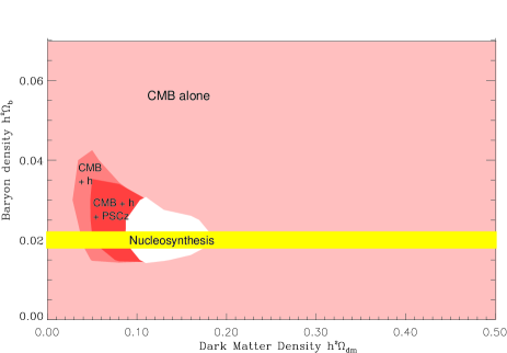
FIG. 6.: Constraints in the $(\omega_{\rm dm},\omega_{\rm b})$-plane. The large pink/grey region is ruled out by CMB data alone at 95% confidence. The two smaller shaded regions become excluded when imposing additional constraints from Hubble constant measurements ($h=0.72\pm 0.08$) and PSCz galaxy clustering. The yellow/light grey band shows the BBN constraints from [57]. The model best fitting the CMB+PSCz+$h$ constraints has $\chi^{2}\approx 126$ for $127$ degrees of freedom.

D Matter budget

We will now investigate the parameter constraints in more detail, exploring which conclusions come from what assumptions. This subsection is centered around the cosmic matter budget (the densities of baryons, cold dark matter, hot dark matter, dark energy and curvature) — we return to the inflationary parameters $n_{s}$, $n_{t}$ and $r$ in the next subsection.

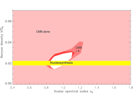
FIG. 7.: Constraints in the $(n_{s},\omega_{\rm b})$-plane. The yellow/light gray band shows the BBN constraints from [57].

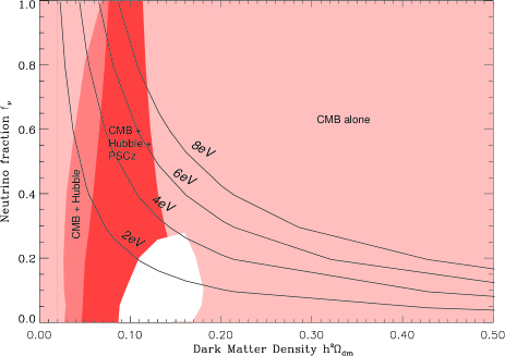
FIG. 8.: Constraints in the $(\omega_{\rm dm},f_{\nu})$-plane. The four curves show contours of constant neutrino mass sum.

1 Constraints from CMB alone

Figures 6, 7 and 8 summarize some of the key 2-dimensional constraints on the matter budget. It is seen that the CMB data alone are now for the first time (compare, eg, [50]) powerful enough to close off bounded regions in these planes. The low second acoustic peak inferred from the first Antarctic BOOMERaNG results [61] was still consistent with a purely baryonic Universe, prompting speculation [62] that an alternative theory of gravity might be able to eliminate the need to for dark matter altogether. Since the more accurate measurements of the second peak height from the new BOOMERaNG, DASI and Maxima data give a higher value, even the CMB alone now requires a non-zero amount of dark matter, at least at modest significance.

The increased second peak height is also seen to resolve a second hot discussion topic of the past year: the CMB lower limit on the baryon density has now dropped down in beautiful agreement with the BBN prediction.

FIG. 9.: The main remaining CMB degeneracy. The three solid curves show the best fit models for CMB alone subject to the constraint $\omega_{\rm b}=0.02$ (red), $\omega_{\rm b}=0.03$ (green) and $\omega_{\rm b}=0.04$ (blue), spanning the “banana” allowed by the CMB in Figure 7. Dashed curves show the scalar and tensor contributions. All models have $\tau=f_{\nu}=0$. The parameters ${\bf p}\equiv(\Omega_{\rm k},\Omega_{\Lambda},\omega_{\rm dm},\omega_{\rm b},n_{s},n_{t})$ are $(-0.043,0.461,0.116,0.020,0.924,0.982)$, $(-0.134,0.799,0.050,0.030,1.200,0.884)$ and
$(-0.160,0.840,0.043,0.040,1.401,0.955)$, respectively.

A third noteworthy result is that the allowed region in our 11-dimensional space is shaped like a long and skinny rather one-dimensional tube. This is seen clearly in the projection onto the $(n_{s},\omega_{\rm b})$ plane in Figure 7. The physics underlying this CMB degeneracy is illustrated in Figure 9. Starting in the generally favored (white) region of Figure 7 and moving up to the right, the Universe becomes more and more closed ($\Omega_{\rm k}$ decreases to negative values), which would on its own shift the acoustic peaks too far to the left. This is compensated by reducing the density of dark matter $\omega_{\rm dm}$ and increasing the dark energy density $\Omega_{\Lambda}$ and the power spectrum tilt $n_{s}$ so that the peak location stays essentially fixed. Through a rather spurious coincidence, the resulting changes in the various peak heights relative to the COBE scale can be almost perfectly reversed by increasing the baryon density and adding substantial amounts of gravity waves. This is in essence the familiar $(\Omega_{\rm k},\Omega_{\Lambda})$ angular distance degeneracy described in many parameter forecasting papers [63, 64], with the extra twist that changing $\omega_{\rm b}$, $\omega_{\rm dm}$, $n_{s}$ and $r$ as well helps minimize the change in the late integrated Sachs-Wolfe effect on COBE scales.

2 Breaking the CMB degeneracy

Since this degeneracy involves so many parameters, prior constraints on any one of them will help break it. In particular, the reason that this degeneracy is not as prominent in the recent analyses by the BOOMERaNG [1], DASI [29] and Maxima [30] teams is because they all assumed negligible gravity waves, $r=0$.

Since the Hubble parameter is given by

$$h=\sqrt{\omega_{\rm dm}+\omega_{\rm b}\over 1-\Omega_{\rm k}-\Omega_{\Lambda}},$$ (10)

it decreases sharply as one moves along the degeneracy track, dropping as low as $0.3$ at the upper right endpoint in Figure 7. Imposing the prior $h=0.72\pm 0.08$ therefore shrinks the allowed 11-dimensional region substantially, among other things tightening the lower limit on dark matter in Figure 6 and the upper limit on baryons in Figure 7.

Because of its sensitivity to $n_{s}$ and $\omega_{\rm dm}$ in particular, our galaxy clustering data (the PSCz power spectrum) is seen to break this CMB degeneracy completely, shrinking the allowed CMB “bananas” to almost round regions in Figure 6 and Figure 7. The effect of adding PSCz is particularly dramatic in Figure 8, since CMB alone has almost no sensitivity to the neutrino fraction, whereas increasing $f_{\nu}$ provides a strong suppression of the galaxy power spectrum on small scales.

The model best fitting the CMB+PSCz+$h$ constraints has $\chi^{2}\approx 126$ for $105+32+1-11=127$ degrees of freedom. The effective number of degrees of freedom might be a few larger than this, since some of the 11 parameters had little effect, but even if we ignore this, all fits are good in the sense of giving reduced $\chi^{2}$-values of order unity.

Adding our additional priors $\omega_{\rm b}=0.02$, $\tau=0$, $\Omega_{\rm k}=0$ and $r=0$ cause little further change, since they are all consistent with the favored results and there are no major degeneracies left to break.

Adding our Ly$\alpha$F data produced effects quite similar to those of adding PSCz: breaking the CMB degeneracy and favoring a flat, roughly scale-invariant Universe. We have chosen to highlight the effects of the PSCz data rather those of the Ly$\alpha$F data in the figures since we found its overall constraining power on parameters to be slightly stronger. For instance, the CMB+Ly$\alpha$F constraints on tilt, curvature and baryon density are $0.91^{+0.14}_{-0.10}$, $-0.03^{+0.07}_{-0.22}$ and $0.021^{+0.008}_{-0.005}$, respectively. Overall, the PSCz and Ly$\alpha$F were found to be strikingly consistent in pulling the CMB in the same direction, as was also found in [14]. Augmenting the CMB+PSCz data with the 13 Ly$\alpha$F points increased the $\chi^{2}$ for the best fit model by only 10, and the good agreement between the galaxy and Ly$\alpha$F can also be seen visually, in Figure 10.

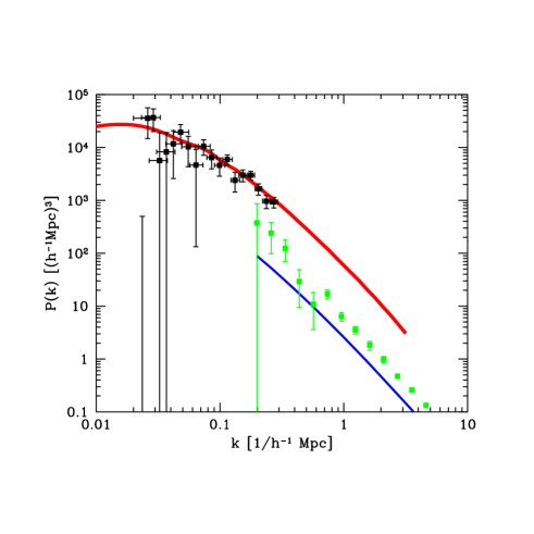
FIG. 10.: The model best fitting the CMB, LSS and Ly$\alpha$F data with $h$ and $f_{\nu}$ priors is shown together with the two data sets. The red and blue curves are the model predictions for the LSS and Ly$\alpha$F data, respectively. The blue curve is simply the red one shifted vertically and horizontally to account for the fluctuation growth and Hubble parameter shift between $z\sim 2.72$ and the present epoch. The overall calibration uncertainty in the Ly$\alpha$F data is seen to let the model prediction lie below the data by a constant factor.

We conclude this subsection by summarizing what is obtained by adding successively stronger assumptions as in Table 2.

1. CMB alone now gives constraints on most parameters, but they are generally weak because of the above-mentioned degeneracy.

2. Adding the PSCz galaxy clustering constraints breaks this degeneracy, resulting in tight constraints on everything except the dark energy density $\Omega_{\Lambda}$.

3. Adding the constraint $h=72\pm 8$ finally nails down $\Omega_{\Lambda}$. It also sharpens the limits on $\Omega_{\rm k}$ and $f_{\nu}$. Adding this one constraint raises $\chi^{2}$ by as much as 4 (from 122 to 126), which reflects a slight tension between the $h$-prior and the CMB+PSCz data, which alone prefer the lower range $h=$$0.57^{+.31}_{-.30}$.

4. Adding an $f_{\nu}=0$ prior boosts $\chi^{2}$ only by 0.1, further sharpening the $\Omega_{\rm k}$, $\Omega_{\Lambda}$ and $\tau$ constraints slightly, and none of our additional priors (including Ly$\alpha$F) have much of an effect. The only exception is imposing $n_{s}=1$, which is slightly disfavored by the data and raises $\chi^{2}$ by 4.

E Inflationary parameters

We now turn our attention to the parameters associated with inflation. Since space remains perfectly consistent with the inflationary flatness prediction despite the sharp error bar reduction caused by the new latest CMB data ($\Omega_{\rm k}=0.00\pm 0.06$ at 95% for CMB+PSCz+$h$), it is interesting to quantify the constraints on the parameters $n_{s}$, $n_{t}$ and $r$ to see how they compare with the predictions of various models, as has previously been done using earlier CMB data [13, 14, 22].

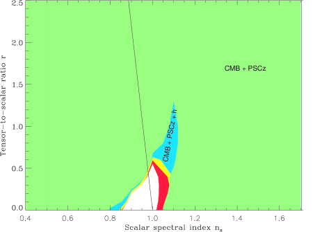
FIG. 11.: Constraints in the $(n_{s},r)$ plane. The large green/light grey region shows the joint constraints from CMB and LSS. The blue/grey region shows the effect of adding the prior $h=0.72\pm 0.08$. The small yellow/light grey region shows the effect of adding $f_{\nu}=0$. The red/dark grey region shows the effect of adding the BBN prior $\omega_{\rm b}=0.02$. The straight line shows the prediction $r=(200/9)(1-n_{s})$ from a power law class of inflation models.

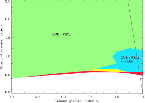
FIG. 12.: Same as previous figure but for the $(n_{t},r)$ plane. The straight line shows the “inflationary consistency relation” $r=-(200/9)n_{t}$.

As discussed in [65], there has been a fair amount of notational confusion in the literature surrounding the tensor-to-scalar ratio $r$. There are two logical ways to define this ratio: either in terms of the fundamental parameters of the power spectrum (or, equivalently, of the inflationary model space), or in terms of the observables, usually the CMB quadrupoles. We adopt the former approach, and define

$$r\equiv{A_{t}\over A_{s}},$$ (11)

where $A_{s}$ and $A_{t}$ are the scalar and tensor fluctuation amplitudes as defined in [65]. For inflation models where the slow-roll approximation is valid, this ratio is related to the tensor tilt $n_{t}$ by the so-called inflationary consistency condition [65, 66]

$$r=-{200\over 9}n_{t}.$$ (12)

A power law class of inflation models (see [13] for a review) make the additional prediction that

$$r\equiv{200\over 9}(1-n_{s}).$$ (13)

i.e., that $n_{s}=n_{t}+1$. (Although the quantity $n_{t}+1$ would be a more natural definition for the tensor spectral index, we will stay true to the astronomical tradition of clinging to silly notation for historical reasons.)

A common alternative definition of the tensor-to-scalar ratio is the quadrupole ratio

$$R\equiv{C^{\rm tensor}_{2}\over C^{\rm scalar}_{2}},$$ (14)

In this case, the inflationary consistency condition is [65]

$$R\approx-{6.93}n_{t}$$ (15)

for the special case where $\Omega_{\rm k}=\Omega_{\Lambda}=0$.

Writing the relation between $R$ and $r$ as

$$r\approx aR,$$ (16)

the proportionality constant $a$ is typically between 2 and 5 — it depends on the values of $\Omega_{\Lambda}$ and $\Omega_{\rm k}$ via the late integrated Sachs-Wolfe effect.

As shown in Table 2, Figure 4 and Figure 5, the data prefers no tensor contribution at all, placing a 95% upper limit $r<0.5$ for the CMB+PSCz+$h$ case. For comparison with prior work, this corresponds to a quadrupole ratio of 0.2 in the sense that this is the quadrupole ratio for the best fit model in our grid with this $r$-value (which is by definition ruled out at exactly the 95% level). For comparison, previous multiparameter analyses incorporating gravity waves [13, 14] found $r<0.3$ using older CMB data and stronger priors.

Figures 11 and 12 show the joint constraints on r with the scalar and tensor tilts, respectively, and allows comparison with the predictions of equations (12) and (13). The constraints in the $(n_{s},r)$ have becomes progressively sharper during the past year [13, 14], and are now gradually becoming quite interesting. In particular, Figure 11 shows that the preference for a slight red-tilt ($n_{s}\sim 0.9$) and low $r$ in the data favors so-called “small-field” models [13].

Figure 12 shows that the holy grail of testing the inflationary consistency relation (12) is still a ways off. As expected, the constraints on the tensor tilt $n_{t}$ are stronger for high tensor normalizations $r$ and vanish completely when $r$ does.

IV Discussion

In Section II, we compared and combined the different CMB experiments, finding that a consistent picture of the angular power spectrum emerged. In Section III, we compared and combined a limited number of cosmological data sets (power spectra from CMB, LSS, Ly$\alpha$F and various priors), finding that a consistent set of cosmological parameters emerged that provided a good fit to this data.

We conclude with some remarks on how these parameter measurements match up with the many other cosmological observations that probe these parameters, focusing on the cosmic matter budget. In light of the checkered history of many cosmological parameters, where tiny quoted error bars have repeatedly masked larger uncertainties about underlying assumptions, such end-to-end consistency checks are crucial. For instance, the Hubble parameter $h$ has dropped by a factor of eight since Hubble’s original paper, the BBN baryon density $\omega_{\rm b}$ has risen by 50% in less than a decade, and the favored value of the cosmological constant $\Omega_{\Lambda}$ has fluctuated wildly at the hands on both theorists and observers.

A Baryon density $\omega_{\rm b}$

The rise of the second peak in the new data has completely eliminated the tension between BBN and CMB, and they two are now in beautiful agreement that the baryon density $\omega_{\rm b}\approx 0.02$. This agreement was noted in the latest team papers as well [1, 29, 30]. That one method involving nuclear physics when the Universe was seconds old and another involving plasma physics more than 100,000 years later give the same answers, despite involving completely different systematics, is a landmark achievement for cosmology. It greatly boosts the credibility of the basic cosmological storyline since the Universe was a split second old. This sudden agreement is all the more impressive given the lack thereof during the past year and the ado this generated.

Consensus has yet to be reached on the second decimal of the BBN predictions, with the value $\omega_{\rm b}=0.023$ from a recent VLT deuterium study [67] lying above the 95% range of [57]. As a reality check, our baryon value also agrees with slightly less accurate estimates of the abundance in the local Universe — e.g., the range $0.007\mathrel{\hbox to0.0pt{\lower 3.0pt\hbox{$\mathchar 536\relax$}\hss}\raise 2.0pt\hbox{$\mathchar 316\relax$}}\Omega_{\rm b}\mathrel{\hbox to0.0pt{\lower 3.0pt\hbox{$\mathchar 536\relax$}\hss}\raise 2.0pt\hbox{$\mathchar 316\relax$}}0.041$ inferred from a low-redshift inventory [68] and the range $0.015\mathrel{\hbox to0.0pt{\lower 3.0pt\hbox{$\mathchar 536\relax$}\hss}\raise 2.0pt\hbox{$\mathchar 316\relax$}}\omega_{\rm b}\mathrel{\hbox to0.0pt{\lower 3.0pt\hbox{$\mathchar 536\relax$}\hss}\raise 2.0pt\hbox{$\mathchar 316\relax$}}0.03$ at redshifts of a few from the Ly$\alpha$ forest [69, 70], although the latter tend to be on the high side. Similarly, the inferred baryon fraction $\omega_{\rm b}/\omega_{\rm dm}\sim 18\%$ agrees with that inferred from galaxy clusters [22, 71], although this match weakly prefers lower $h$-values.

B Dark matter and dark energy density

By now, there are a large number of independent methods for probing the dark matter density $\omega_{\rm dm}$ or the (almost identical) total density, including studies of the cluster abundance at various redshifts [71, 72, 73, 74, 75], mass-to-light ratio techniques [76, 77], the baryon fraction $\Omega_{\rm b}/\Omega_{\rm m}$ from cluster studies [78], cosmic velocity fields and redshift space distortions. Most of these probes do not measure $\omega_{\rm dm}$ directly, but $\Omega_{\rm dm}=\omega_{\rm dm}/h^{2}$ or some combination of this with the fluctuation normalization parameter $\sigma_{8}$. Although each comes with potential systematic errors of its own, and there is still some internal controversy in the velocity and cluster areas [79], they are all broadly consistent with the range $\omega_{\rm dm}=0.09-0.18$ listed in Table 2. Indeed, it is interesting that some of the last evidence supporting $\Omega_{\rm m}\sim 1$ came from velocity fields and redshift distortion studies, and that improved data now gives values as low as in Table 2 from both velocity fields [80, 81] and redshift space distortions [53, 82, 83].

With CMB strongly favoring an essentially flat Universe, the low matter density automatically implies a high dark energy density. As has been discussed in numerous papers (e.g., [1, 19, 50]), there are now independent ways of reaching this conclusion, making it robust to throwing away information on either supernovae 1a [84, 85] or large-scale structure. The BOOMERaNG team [1] argue that even CMB and Hubble constant measurements now favor $\Omega_{\Lambda}>0$ — we have seen that this conclusion hinges on the the important additional assumption of negligible gravity waves.

C Neutrino density

For the neutrino density $\omega_{\nu}$, we are still a far cry from the grand goal of a precision cross-check between cosmological and laboratory measurements, since the two have so far provided only upper and lower limits, respectively. However, the two limits are steadily creeping closer. Atmospheric neutrino oscillations [59] show that there is at least one neutrino (presumably a linear combination of $\nu_{\mu}$ and $\nu_{\tau}$) whose mass exceeds a lower limit somewhere in the range 0.04-0.08 eV [60]. Since

$$\omega_{\nu}\equiv{1\over 94{\rm eV}}\sum_{i}m_{i},$$ (17)

where $m_{i}$ is the mass of the $i$th neutrino, this corresponds to a lower limit $\omega_{\nu}\mathrel{\hbox to0.0pt{\lower 3.0pt\hbox{$\mathchar 536\relax$}\hss}\raise 2.0pt\hbox{$\mathchar 318\relax$}}0.0004-0.0008$, or $f_{\nu}\mathrel{\hbox to0.0pt{\lower 3.0pt\hbox{$\mathchar 536\relax$}\hss}\raise 2.0pt\hbox{$\mathchar 318\relax$}}0.003-0.01$, Our constraints (see Figure 8) give $\sum m_{i}<4.2$eV, further sharpening the 5.5 eV limit from a careful analysis of previous cosmological data [86] (see also [22]). The mass of the heaviest neutrino is thus in the range $0.04-4.2$ eV.

Moreover, the mass-splittigs indicated by both solar and atmospheric neutrino data are much smaller than 4.2 eV, suggesting that all three mass eigenstates would need to be almost degenerate for neutrinos to weigh in near our upper limit. This means that the upper limit on the (almost identical) masses of the three neutrino states would be $4.2/3=1.4$ eV.

Note that if, as current data suggests, the mixing between the flavor eigenstates $\nu_{e}$, $\nu_{\mu}$ and $\nu_{\tau}$ is not small, it is inappropriate to identify the three mass-eigenstates $\nu_{1}$, $\nu_{2}$ and $\nu_{3}$ with these flavor eigenstates. For instance, the heaviest eigenstate $\nu_{3}$ is likely to be almost a $50-50$ mixture of $\nu_{\tau}$ and $\nu_{\mu}$. The correct way to phrase our upper limit is therefore as a 1.4 eV upper limit on the the mass of $\nu_{3}$.

Finally, a caveat about non-standard neutrinos is in order. To first order, our cosmological constraint probes only the mass density of neutrinos. Our conversion of this into a limit on the mass sum assumes that the neutrino number density is known and given by the standard model freezeout calculation; 112 cm^-3. In more general scenarios with sterile or otherwise non-standard neutrinos where the freezeout abundance is different, the robust conclusion to take away is simply an upper limit on the total light neutrino mass density of $8.4\times 10^{-28}$kg/m³.

How do our results compare with those of other recent analyses? The analysis most similar to ours is that of the BOOMERaNG team [1]. A detailed numerical comparison of their results with our Table 2 is very encouraging. Despite major differences in both analysis technique (priors, parameter space, marginalization method, etc.) and data used (that analysis was limited to BOOMERAnG and DMR data), both the central values and the error bars are very similar for most parameters when taking into account that they and we quote $1\sigma$ and $2\sigma$ errors, respectively. This indicates that what is being measured is really borne out loud and clear by the data in a way that is robust towards data selection or analysis details. Perhaps we are inevitably approaching the dreaded day when not only cosmology is consistent, but cosmologists are as well.

The authors wish to thank Angélica de Oliveira-Costa, Alexander Friedland, David Hogg, Andrew Jaffe, Josh Klein, John Kovac, Pat McDonald, Jim Peebles, Clem Pryke, Adam Riess, Dominik Schwarz, George Smoot, David Weinberg, and especially Andrew Hamilton for helpful comments and suggestions. Support for this work was provided by NSF grant AST00-71213, NASA grants NAG5-9194 and NAG5-11099, the University of Pennsylvania Research Foundation, the Zaccheus Daniel Foundation and two awards from the David and Lucile Packard Foundation.

A Linearized modeling of calibration and beam errors

This appendix describes our modeling of the four terms of the error matrix from equation (2), assuming that all relative errors are small ($\ll 1$).

${\bf N}^{\rm(meas)}$ reflects the part of the errors which are uncorrelated between the different experiments and is due to detector noise and sample variance. We approximate it by

$${\bf N}^{\rm(meas)}_{ij}\equiv\delta_{ij}\sigma_{i}^{2},$$ (A1)

where $\sigma_{i}$ is defined as the average of the upper and lower error bars quoted for $d_{i}\equiv\delta T^{2}$.

The last three terms in equation (2) reflect correlations between measurements due to calibration and beam errors. As in [31, 42], ${\bf N}^{\rm(ical)}$ is the part specific to a single multi-band experiment and ${\bf N}^{\rm(scal)}$ is the part that is correlated with other experiments that are calibrated off of the same (slightly uncertain) source. TOCO, MSAM, CBI and BOOMERaNG all calibrate off of Jupiter. To be conservative, we assume that the full 5% calibration uncertainty from Jupiter’s antenna temperature is shared by these experiment. The true correlation should be lower, since the four experiments observed Jupiter at different frequencies. The remaining multi-band experiments in Figure 1 should not have any such inter-experiment correlations. This contribution to the noise matrix is therefore

$${\bf N}^{\rm(scal)}_{ij}\equiv(2s_{ij})^{2}y_{i}y_{j},$$ (A2)

where

$$s_{ij}=\cases{5\%&if $i$ and $j$ refer to a Jupiter-calibrated point,\cr 0&otherwise.\cr}$$ (A3)

The factor of 2 in equation (A2) stems from the fact that the percentage error on $\delta T_{i}^{2}$ is roughly twice that for $\delta T_{i}$ as long as it is small. We simply use the observed values for $y_{i}$ in this expression.

Similarly, the remaining calibration term is

$${\bf N}^{\rm(ical)}_{ij}\equiv(2r_{ij})^{2}y_{i}y_{j},$$ (A4)

where $r_{ij}=0$ if $i$ and $j$ refer to different experiments. If band powers $i$ and $j$ are from the same experiment, then $r_{ij}$ is the quoted calibration error with the source contribution $s_{ij}$ subtracted off in quadrature. We use 10% for QMASK, 14% for Python V, 8% for Viper, 8.7% for Toco 97, 6.2% for Toco 98, 10% for QMASK, 6.4% for BOOM97, 10% for BOOM98, 4% for Maxima and 4% for DASI.

A Gaussian beam of standard deviation $\theta$ suppresses power by a factor well approximated by $e^{(\l\theta)^{2}}$. Taylor expanding this expression shows that a small beam error $\Delta\theta$ causes the power to be mis-estimated by a percentage $2\l^{2}\theta\Delta\theta$. Defining

$$b_{i}\equiv 2{\Delta\theta_{i}\over\theta_{i}}\left({\l\theta_{i}}\right)^{2}y_{i},$$ (A5)

we can therefore write the beam error as

$${\bf N}^{\rm(beam)}_{ij}=b_{i}b_{j}$$ (A6)

when $i$ and $j$ refer to the same experiment, zero otherwise. We use this approximation for BOOM98, where $\theta=12.9^{\prime}/c$, $\delta\theta=1.4^{\prime}/c$, and $c=\sqrt{8\ln 2}$ is the familiar FWHM conversion factor. The other experiment reporting important beam uncertainties is Maxima, for which we use the $b_{i}$-coefficients published in [3] in place of the approximation of equation (A5).

REFERENCES

- [1] C. B. Netterfield, astro-ph/0104460 (2001).
- [2] N. W. Halverson, astro-ph/0104489 (2001).
- [3] A. T. Lee et al., astro-ph/0104459 (2001).
- [4] P. J. E Peebles and J. T. Yu, ApJ 162, 815 (1970).
- [5] R. Sunyaev and Ya. Zeldovich, Astrophys. & Space Sci. 7, 3 (1970).
- [6] A. E. Lange et al., Phys. Rev. D 63, 042001 (2001).
- [7] M. Tegmark and M. Zaldarriaga, Phys. Rev. Lett. 85, 2240 (2000).
- [8] A. Balbi et al., ApJL 545, L1 (2000).
- [9] W. Hu, M. Fukugita, M. Zaldarriaga, and M. Tegmark, ApJ 549, 669 (2001).
- [10] A. Jaffe et al., Phys. Rev. Lett. 86, 3475 (2000).
- [11] T. Padmanabhan and S. K. Sethi, ApJ 555, 125 (2001).
- [12] C. H. Lineweaver, astro-ph/0011448 (2000).
- [13] W. H. Kinney, A. Melchiorri, and A. Riotto, Phys. Rev. D 63, 23505 (2001).
- [14] S. Hannestad, S. H. Hansen, F. L. Villante, and A. J. S Hamilton, astro-ph/0103047 (2001).
- [15] S. Hannestad, Phys. Rev. D 64, 083002 (2001).
- [16] L. M. Griffiths, A. Melchiorri, and J. Silk, ApJ 553, L5 (2001).
- [17] J. Phillips, D. H. Weinberg, R. A. C Croft, L. Hernquist, N. Katz, M. Pettini, ApJ 560, 15 (2001).
- [18] J. R. Bond et al., astro-ph/0011378 (2000).
- [19] N. Bahcall, J. P. Ostriker, S. Perlmutter, and P. J. Steinhardt, Science 284, 1481 (1999).
- [20] B. Novosyadlyj, R. Durrer, S. Gottlöber, V. N. Lukash, and S. Apunevych, A&A 356, 418 (2000).
- [21] B. Novosyadlyj, R. Durrer, S. Gottlöber, V. N. Lukash, and S. Apunevych, astro-ph/0002522 (2000).
- [22] R. Durrer and B. Novosyadlyj, MNRAS 324, 560 (2001).
- [23] S. L. Bridle et al., MNRAS 321, 333 (2001).
- [24] M. S. Turner, astro-ph/0106035 (2001).
- [25] G. Holder, Z. Haiman, and J. Mohr, astro-ph/0105396 (2001).
- [26] S. Padin et al., ApJL 549, L1 (2001).
- [27] G. Efstathiou et al., astro-ph/0109152 (2001).
- [28] O. Lahav et al., astro-ph/0112162 (2001).
- [29] C. Pryke et al., astro-ph/0104490 (2001).
- [30] R. Stompor et al., astro-ph/010506 (2001).
- [31] M. Tegmark and M. Zaldarriaga, ApJ 544, 30 (2000).
- [32] Y. Xu, M. Tegmark, A. de Oliveira-Costa, M. Devlin, T. Herbig, A. D. Miller, C. B. Netterfield, and L. A. Page, Phys. Rev. D 63, 103002 (2001).
- [33] C. B. Netterfield, M. J. Devlin, N. Jarosik, L. A. Page, and E. J. Wollack, ApJ 474, 47 (1997).
- [34] M. Devlin, A. de Oliveira-Costa, T. Herbig, A. D. Miller, C. B. Netterfield, L. A. Page, and M. Tegmark, ApJL 509, L77 (1998).
- [35] T. Herbig et al., ApJL 509, L73 (1998).
- [36] A. de Oliveira-Costa, M. Devlin, T. Herbig, A. D. Miller, C. B. Netterfield, L. A. Page, and M. Tegmark, ApJL 509, L77 (1998).
- [37] E. Gawiser and J. Silk, Phys. Rept. 333-334, 245 (2000).
- [38] C. L. Bennett et al., ApJ 464, L1 (1996).
- [39] Y. Xu, M. Tegmark, and A. de Oliveira-Costa, astro-ph/0104419 (2001).
- [40] D. Scott, J. Silk, and M. White, Science 268, 829 (1995).
- [41] E. Pierpaoli, D. Scott, and M. White, Mod. Phys. Lett. A 15, 1357 (2000).
- [42] L. Knox and L. Page, Phys. Rev. Lett. 85, 1366 (2000).
- [43] J. R. Bond, A. H. Jaffe, and L. E. Knox, ApJ 533, 19 (2000).
- [44] M. Tegmark, ApJ 480, L87 (1997).
- [45] E. L. Wright, astro-ph/9612006 (1996).
- [46] M. Tegmark, ApJ 519, 513 (1999).
- [47] M. Tegmark and B. C. Bromley, ApJL 518, L69 (1999).
- [48] M. Seaborne et al., MNRAS 309, 89 (1999).
- [49] W. H. Press, astro-ph/9604126: (1996).
- [50] M. Tegmark, M. Zaldarriaga, and A. J. S Hamilton, Phys. Rev. D 63, 43007 (2001).
- [51] A. Taruya, H. Magara, Yi. P. Jing, and Y. Suto, PASJ 53, 155 (2001).
- [52] W. Saunders et al., MNRAS 317, 55 (2000).
- [53] A. J. S Hamilton, M. Tegmark, and N. Padmanabhan, MNRAS 317, L23 (2000).
- [54] A. C. Croft et al., astro-ph/0012324 (2000).
- [55] P. McDonald, J. Miralda-Escudé, M. Rauch, W. L. W Sargent, T. A. Barlow, R. Cen, and J. P. Ostriker, ApJ 543, 1 (2000).
- [56] A. J. S Hamilton, MNRAS 322, 419 (2001).
- [57] S. Burles, K. M. Nollett, and M. S. Turner, ApJ 552, L1 (2001).
- [58] W. L. Freedman et al., ApJ 553, 47 (2001).
- [59] Y. Fukuda et al., Phys. Rev. Lett. 82, 1810 (1999).
- [60] J. W. F Valle, astro-ph/0104085 (2001).
- [61] P. de Bernardis et al., Nature 404, 955 (2000).
- [62] S. S. McGaugh, ApJL 541, L33 (2000).
- [63] J. R. Bond, G. Efstathiou, and M. Tegmark, MNRAS 291, L33 (1997).
- [64] D. J. Eisenstein, W. Hu, and M. Tegmark, ApJ 518, 2 (1999).
- [65] J. Martin and D. Schwarz, Phys.Rev. D 62, 103520 (2000).
- [66] A. R. Liddle and D. H. Lyth, Phys. Lett. B 291, 391 (1992).
- [67] S. D’Odorico, M. Dessauges-Zavadsky, and P. Molaro, A&A 368, L21 (2001).
- [68] M. Fukugita, C. J. Hogan, and P. J. E Peebles, ApJ 503, 518 (1998).
- [69] M. Rauch et al., ApJ 489, 7 (1997).
- [70] L. Hui, Z. Haiman, M. Zaldarriaga, and T. Alexander, ApJ 564, 525 (2002).
- [71] J. J. Mohr, Z. Haiman, and G. P. Holder, astro-ph/0004244 (2000).
- [72] J. M. Diego et al., astro-ph/0104217 (2001).
- [73] N. A. Bahcall and X. Fan, ApJ 504, 1 (1998).
- [74] V. R. Eke, S. Cole, C. S. Frenk, and J. P. Henry, MNRAS 298, 1145 (1998).
- [75] J. P. Henry, ApJ 534, 565 (2000).
- [76] N. A. Bahcall et al., ApJ 541, 1 (2000).
- [77] R. G. Carlberg et al., ApJ 516, 552 (1999).
- [78] L. Grego et al., ApJ 552, 2 (2001).
- [79] A. R. Liddle and P. T. P Viana, MNRAS 303, 535 (1999).
- [80] I. Zehavi and A. Dekel, Nature 401, 252 (1999).
- [81] A. Nusser, L. N. da Costa, E. Branchini, M. Bernardi, M. V. Alonso, G. Wegnerary, C. N. A Willmer, P. S. Pellegrini, MNRAS 320, L21 (2001).
- [82] H. Valentine, W. Saunders, and A. Taylor, MNRAS 319, L13 (2000).
- [83] J. A. Peacock et al., Nature 410, 169 (2001).
- [84] S. Perlmutter et al., Nature 391, 51 (1998).
- [85] A. G. Riess et al., Astron. J. 116, 1009 (1998).
- [86] R. A. C Croft, W. Hu, and R. Davé, Phys. Rev. Lett. 83, 1092 (1999).