Geodetic Precession in Binary Neutron Stars

Abstract

The most recent evidence for geodetic precession observed in binary radio pulsars is presented and discussed. It is demonstrated how an analysis of these results can be used to study theories of gravity, stellar evolution and pulsar emission theory. In order to highlight the observational strategies, an overview of the applied techniques is given.

1 Introduction

The discovery of pulsars in 1967[1] marked the beginning of a new era in astrophysics. Besides studying pulsars as fascinating astrophysical objects in their own right, these sources serve as invaluable tools in the research of a large variety of physical and astrophysical problems. Studied subjects range from plasma and solid-state physics under extreme conditions to investigations of the interstellar medium. One can study stellar and binary evolution as well as high precision astrometry and planetary ephemerides. Applications are found in cosmology, quantum physics and, of course, in gravitational physics. The latter application became possible with the discovery of the first binary pulsar by Hulse & Taylor in 1974[2]. As they immediately realized, a pulsar in a binary orbit represents a highly stable and accurate clock orbiting in the gravitational field of (usually) compact stars. They were fortunate to discover in PSR B1913+16 the first double neutron star system. These systems are doubly rare because they are formed less often and also since they are more difficult to detect (significant Doppler smearing of the pulse signal occurs when the orbits are less than about 1 day).

Meanwhile many more binary pulsars have been discovered. At the time of writing about 5%, or 70 pulsars out of more than 1300 known, are in binary systems. Three pulsars are in orbit with normal or giant stars, and two pulsars are members of planetary systems. The rest of the binary pulsar population has compact stars, i.e. white dwarfs or neutron stars, as companions. The majority are orbited by white dwarfs of typically $0.2M_{\odot}$, although there is a small but growing population of heavy white-dwarf companions[3, 4, 5]. Pulsar–white-dwarf systems have been used to perform unique tests of certain aspects of gravitational theories[6], for instance testing the existence of gravitational dipole radiation as predicted by many alternative theories of gravity[7] or the violation of the strong equivalence principle[8]. However, for tests of theories of gravity in a strong field limit, observations of double neutron star systems still yield the most exciting results.

Only five double neutron star systems (DNSs) are known. Orbital periods range from 7.7 hours for PSR B1913+16[2] to 18.8 days in the case of the most recent discovery, PSR J1811$-$1736[9]. Presently, two of the five DNSs allow the determination of more than two post-keplerian (PK) parameters. The PK parameters describe relativistic corrections to Newtonian physics, represented by the five standard Keplerian parameters, and can be written as functions of the pulsar and companion masses, $m_{p}$ and $m_{c}$, and the Keplerian parameters. These functions will differ for different theories of gravity, but when Keplerian and PK parameters are measured by observations in a manner independent of a particular theory of gravity, the observations can be compared to theory[10]. If two PK parameters are measured, a given theory of gravity will produce values for the pulsar and companion mass. More generally, a measurement of $n$ PK parameters describes $n$ curves in a two dimensional $m_{p}$-$m_{c}$ plane whose shape and position depend on the theory of gravity being applied. If the chosen theory is an accurate and adequate description of the physics, all $n$ curves should meet in a single point. A measurement of at least three PK parameters hence allows one to perform tests of gravitational theories

The measurement of PK parameters has been possible thanks to a powerful technique called pulsar timing. When giant radio telescopes are used to measure the arrival time of photons emitted by the pulsar, a breath-taking accuracy can be achieved in experiments which are impossible to perform on Earth or in the solar system. For details, we refer to the contribution by Stairs (these proceedings) and to reviews like that of Backer & Hellings (1986)[11]. Despite the remarkable successes achieved with pulsar timing, one particular aspect of gravitational physics can only be studied adequately if the structure of the received pulses itself is analysed carefully.

In general relativity, the proper reference frame of a freely falling object suffers a precession with respect to a distant observer, called geodetic precession. A direct measurement of this effect is the scientific goal of the Gravity Probe-B satellite experiment (see Everitt, these proceedings). In a binary pulsar system this geodetic precession leads to a relativistic spin-orbit coupling, analogous to spin-orbit coupling in atomic physics. As a consequence, the pulsar spin precesses about the total angular momentum, changing the relative orientation of the pulsar towards Earth. In such a case, we should expect a change in the radio emission received from the pulsar, as first proposed by Damour & Ruffini[12] very soon after the discovery of PSR B1913+16. Hence, in contrast to “only” accurately registering the arrival times of pulsar signals, we are even more interested in the emission properties when we want to study geodetic precession.

In this paper we will summarize how to study geodetic precession in binary pulsars. As we have to analyse the emission properties of radio pulsars, we first provide a brief introduction into pulsars and their radiation properties. We report observations for PSR B1913+16 and discuss models used to describe detected pulse shape changes. We demonstrate how information about the system geometry can be used to learn about the effects of asymmetric supernova explosions and “kicks” imparted to newly born neutron stars. Observations of two more binary pulsars, PSRs B1534+12 and J1141$-$6545 are discussed as they provide more evidence for geodetic precession.

Table 1: Selected parameters for the pulsars discussed. Uncertainties in the last digits are quoted in brackets.

	PSR B1913+161	PSR B1534+122	PSR J1141$-$65453
$P$ (ms)	59.029997929613(7)	37.9044403237164332(10)	393.897833900(3)
$P_{b}$ (d)	0.322997462736(7)	0.4207373013796296135(10)	0.197650966(6)
$e$	0.6171308(4)	0.2736777(5)	0.171881(9)
$a\;\sin i$ (lt-s)	2.3417592(19)	3.729463(3)	1.859470(14)
$m_{p}$ (M⊙)	1.4411(7)	1.339(3)	?
$m_{c}$ (M⊙)	1.3879(7)	1.339(3)	?

¹Taylor & Weisberg (1989), ²Stairs et al. (1998), ³Kaspi et al. (2000)

2 Pulsars

2.1 The Clock

Pulsars are rotating neutron stars. From timing measurements of binary radio pulsars we determine the masses of pulsars to be within a quite narrow range of $1.35\pm 0.04M_{\odot}$[13]. Model calculations involving different equations of state produce results for the size of a neutron star quite similar to the very first calculations by Oppenheimer & Volkoff (1939)[14], i.e. about 20 km in diameter. Such sizes are consistent with independent estimates derived from modelling light-curves and luminosities of pulsars observed in X-rays, e.g. for PSR J0437$-$4715[15].

These massive and compact stars rotate with typical periods of about 0.6 s for “normal” pulsars, and periods as low as 1.56 ms for millisecond (“recycled”) pulsars (cf. Fig. 10). Considering that this smallest rotational period for PSR B1937+21 corresponds to more than 38000(!) revolutions per minute makes the large stability of pulsars as clocks easy to understand.

Typical magnetic field strengths at neutron star surfaces are of order $10^{12}$ G. By comparison, the Earth’s magnetic field is only 1 G. We can infer these field strengths from the slow increase in pulse period due to the loss of rotational energy by the emission of magnetic dipole radiation, or more directly from synchrotron lines in X-ray spectra of X-ray pulsars[16].

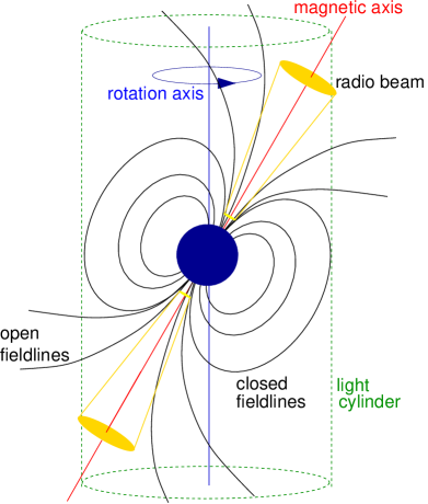
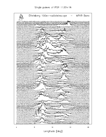
Figure 1: left) A pulsar is a rotating, highly magnetised neutron star. A radio beam centred on the magnetic axis is created at some distance to the pulsar. The tilt between the rotation and magnetic axes makes the pulsar in effect a cosmic lighthouse when the beam sweeps around in space; right) while individual pulses vary in shapes and strength (zoomed in,top), average profiles are stable (full profile, bottom). The typical pulse duty cycle is only $\sim$4%.

2.2 The Clockwork

The tick of the pulsar clock is provided by a narrow radio beam centred on the magnetic axis of the pulsar, which is inclined to the rotation axis (see Fig. 1). If the pulsar beam is directed towards Earth once per rotation, radio telescopes on Earth may be able to pick up a pulsed radio signal. This periodic beacon sent by the pulsar clock is usually rather weak due to the distance of the pulsar, but also due to the small size of the emission region, which we expect to be only a few hundred km across[17]. Nevertheless, the radio emission is actually rather intense as we measure brightness temperatures exceeding $10^{30}$ K, which we can only explain by assuming a coherent emission mechanism. After 35 years of pulsar research, the details of the actual emission process still elude us, but at least we have some basic understanding sufficient to perform the experiments described later.

As the neutron star rotates with its magnetic field, an induced electric quadrupole field pulls out easily charges from the stellar surface (the electrical force exceeds the gravitational force by a factor of $10^{12}$!), surrounding the pulsar with dense plasma. The magnetic field forces the plasma to co-rotate with the pulsar like a rigid body. This co-rotating magnetosphere can only extend up to a distance where the co-rotation velocity reaches the speed of light. This distance defines the so-called light cylinder which separates the magnetic field lines into two distinct groups, i.e. open and closed field lines. Closed field lines are those which close within the light cylinder, while open field lines would close outside. The plasma on the closed field lines is trapped and will co-rotate with the pulsar forever. In contrast, plasma on the open field lines can reach highly relativistic velocities and can leave the magnetosphere, creating the observed radio beam at a distance of a few tens to hundreds of km above the pulsar surface (see Fig. 1).

2.3 The ticks

Individual Pulses and Average Pulse Profiles

Individual pulses reflect the instantaneous plasma processes in the pulsar magnetosphere at the moment when the beam is directed towards Earth. The dynamics of these processes results in often seemingly random individual pulses, in particular when viewed with high time resolution (see Fig. 1). Despite this variety displayed by the single pulses, the mean pulse shape computed by averaging a few hundreds to few thousands of pulses is incredibly stable[18]. In contrast to the snapshot provided by the individual pulses, the average pulse shape, or pulse profile, can be considered as a long-exposure picture, revealing the global circumstances in the magnetosphere. These are mostly determined by geometrical factors and the strong magnetic field, leading to very stable pulse profiles. Apart from a distinct evolution with radio frequency, the same profiles are obtained, no matter where and when the pulses used to compute the average have been observed.

Beam Shapes

The observed pulse profiles show a large variety of shapes. Although each pulsar exhibits a slightly different profile – almost like a unique fingerprint – a systematic pattern can be recognized. The most simple model successfully describing the beam shapes is that of a hollow cone of emission[22]. It is based on the idea that the outermost open field lines, which show the largest curvature among the “emitting field lines”, should be associated with the strongest emission, leading naturally to a cone-like structure. Observations show that this picture is oversimplified, since we also often observe components near the centre of the cone, a so called core component, in particular at lower frequencies. However, the combination of a hollow cone with a core component can be successfully applied to understand the vast majority of pulsar profiles[23, 24, 25]. Depending on the way how our line-of-sight cuts the emission cone, different pulse profiles are observed (Fig. 2).

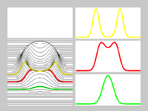
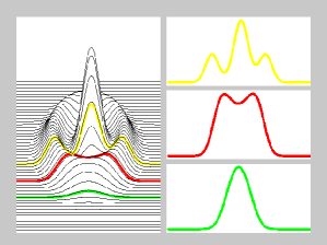
Figure 2: left) Hollow cone model to explain the observed pulse profiles as different cuts through the emission beam; right) very often an additional “core” component is observed near the centre of the beam, in particular at low frequencies.

Polarisation — Signatures of Geometry

An important and most useful property of pulsar radio emission is its typical high degree of polarisation. The radiation is often 100% elliptically polarized, and it is usual practice to separate the polarisation into linearly and circularly polarized components. The linear component is often the far dominating one, although pulsars with circular components as strong as 30% or more are not uncommon. The degree of polarisation decreases with increasing frequency, leaving pulsars more or less completely de-polarized at high frequencies[26]. At low frequencies, however, the polarisation serves as a useful diagnostic tool, both to measure the magnetic field of the ionized interstellar medium and, in particular for our purposes, to obtain information about the viewing geometry.

The strong coupling of the outwards-moving plasma to the magnetic field lines in the pulsar magnetosphere has the effect that the plane of polarisation of the linear component is determined by the plane embedding the corresponding field line. The observed position angle (PA) of the linear polarisation is then given by the projection of this direction onto our line-of-sight. The result is an S-like curve of the PA whose shape depends on the angle between the rotation and magnetic axes as well as on the distance of our line-of-sight to the magnetic pole. If our line-of-sight cuts the emission beam close to the magnetic axis, the PA changes rapidly when crossing the centre of the beam. If we are cutting the cone further away from the pole, the transition is much smoother and the PA swing much flatter.

By measuring the polarisation characteristics of a pulsar, we can in principle win information about the pulsar’s orientation towards us. In practice, fitting this rotating vector model[27] (RVM) often turns out to be difficult. Although the majority of observed PA swings can be well described by the RVM after correcting for sometimes occurring orthogonal modes (i.e. jumps of the PA by nearly 90^∘ which are probably magnetospheric propagation effects), the uncertainties in the obtained angles representing the geometry are typically large. The reason is not a failure of the model, but simply the small size of beam of most pulsars, which provides constraints to the fit for only the small fraction of the pulse period when the pulse is actually observed, which is typically only 4%.

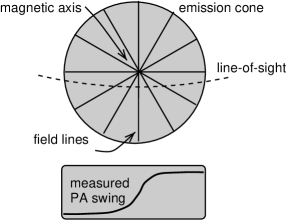
Figure 3: left) Pulsar emission is often highly polarized. The PA of the linear component usually performs an S-like swing across the profile, right) the change in PA can be understood as a projection of the field line direction onto our line-of-sight.

The geometrical origin of the PA swing across the pulse is impressively demonstrated by its independence upon observing frequency. Even if the results of a RVM fit to the PA data are not very well constrained, an observed change in the swing curve will immediately indicate a change in viewing geometry.

3 Evidence for Geodetic Precession — Part I.

Immediately after the discovery of the 59-ms binary pulsar PSR B1913+16 it was realized that the system should exhibit a measurable amount of geodetic precession if the pulsar spin axis is misaligned with respect to the orbital angular momentum vector [12, 28, 29, 30] We will discuss the possible origin for a misalignment of the spin vectors later and first concentrate on the expected observational consequences.

3.1 Precession rate

The precession rate is given by[29, 31]

$$\Omega_{p}=\left(\frac{2\pi}{P_{b}}\right)^{5/3}\cdot T_{\odot}^{2/3}\cdot\frac{m_{c}(4m_{p}+3m_{c})}{2(m_{p}+m_{c})^{4/3}}\cdot\frac{1}{1-e^{2}}$$ (1)

where $P_{b}$ is the period and $e$ the eccentricity of the orbit. We express the masses $m_{p}$ and $m_{c}$ in units of solar masses ($M_{\odot}$) and the define the constant $T_{\odot}=GM_{\odot}/c^{3}=4.925490947\mu$s. $G$ denotes the Newtonian constant of gravity and $c$ the speed of light.

The values for the orbital period and the eccentricity of the PSR B1913+16 system can be obtained from timing observations (see Table 1). These observations have also resulted in the measurements of three PK parameters, providing the most stringent test of gravitational theories in the strong field limit so far[32, 33, 34]. General relativity has passed all these tests with flying colours. We therefore have safe and accurate measurements for the masses of both pulsar and its companion: $m_{p}=1.4411\pm 0.0007$ and $m_{c}=1.3879\pm 0.0007$. (Strictly speaking these observed masses differ from the intrinsic ones by an unmeasurable Doppler factor due a radial velocity, which cannot be determined from timing measurements. We can safely neglect this small difference here.) Using these values we obtain a precession rate of $\Omega_{p}=1.21$ deg yr^-1. Since the orbital angular momentum is much larger than the pulsar spin, the orbital spin practically represents a fixed direction in space, defined by the orbital plane of the binary system. Given the calculated precession rate, it takes 297.5 years for the pulsar spin vector to precess around it.

3.2 First Signs – First Riddles

As a result of the precession the angle between the pulsar spin axis and our line-of-sight should change with time, so that different portions of the emission beam are observed. Consequently, one expects changes in the measured pulse shape, in particular in the profile width, as a function of time (see Fig. 4). In the extreme case, the precession may move the beam out of our line-of-sight and the pulsar may disappear from the sky until it becomes visible again.

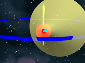
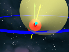
Figure 4: Precession changes the cut of our line-of-sight (indicated by circle) through the emission cone. The consequence should be a change in the width and possibly also shape of the pulse profile. Since the distance between line-of-sight and magnetic axis is changing, an alteration of the position angle swing is expected.

Since the precession rate predicted by general relativity is reasonably large, the pulse profile was naturally studied closely in order to detect possible changes. Finally, Weisberg et al. (1989, hereafter WRT89)[35], reported a change in the relative amplitude of the two prominent profile components (Fig. 5, left). Analyzing observations made at 1408 MHz from 1981 to 1987, they determined a change in the amplitude ratio of $1.2\pm 0.2$% yr^-1, i.e. a weakening of the leading component.

These first signs of profile changes could be indeed explained by a changing cut through the emission beam and hence as the first evidence for geodetic precession. However, if the emission beam exhibits an overall hollow-cone like shape, one would also expect a change in the separation of the two components rather than only a change in relative intensity. This was not observed. WRT89 determined an upper limit of $\Delta W<0.^{\circ}06$ for a change in component separation in the given time interval. In order to reconcile this constant profile width with the seen amplitude changes, they argued that the beam structure is irregular and patchy rather than cone-like, i.e. similar to models by Lyne & Manchester (1988)[36].

With different cuts through the emission beam, the distance of our line-of-sight to the magnetic axis should also change with time. A change in the PA swing would be expected. Cordes, Wasserman & Blaskiewicz (1990, hereafter CWB90)[37] therefore studied polarisation data of PSR B1913+16 to compare profiles and PA swings obtained at frequencies between 1397 and 1416 MHz from 1985 to 1988. CWB90 neither detected very clear changes in the pulse shape, nor could they find any significant change in the PA swing. CWB90 pointed out that their results and those of WRT89 could be still consistent with a hollow cone emission beam. They proposed that the existence of a core component, which is prominent at lower frequencies[48] (see Fig. 8), is causing the change in the component amplitude ratio. Finally, they suggested that the lack of detected changes in profile width and PA swing was due to a special precession phase at the time of observation.

The situation remained somewhat unsatisfactory. While the amplitude changes detected by WRT89 seemed to be clear indications of the presence of geodetic precession, the actually expected behaviour, i.e. a change in profile width and PA swing, was not observed.

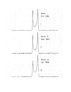
Figure 5: left) Pulse profile of PSR B1913+16 as presented by Taylor & Weisberg (1989). The change in component amplitudes studied by Weisberg & Taylor (1989) is clearly visible, right) profile of B1913+16 in 1995 and component amplitude ratio as presented by Kramer (1998).

3.3 The Times, They are a Changing

In 1994 the pulsar B1913+16 was included in a timing program at the 100-m radio telescope at Effelsberg, which was initiated to take over the regular timing of millisecond pulsars during the upgrade of the 300-m Arecibo telescope in Puerto Rico[39]. The analysis of profiles measured between 1994 and 1998 by Kramer (1998)[40] revealed that the profile components were still changing their relative amplitude, consistent with the rate first determined by WRT89 (see Fig. 5). Even more interesting, however, was the final detection of a small but significant change in the separation of the components (see Fig. 6). In order to model the long-expected decreasing width of the profile, two simple assumptions were made, i.e. those of a circular hollow cone-like beam and a precession rate as predicted by general relativity. Both well justified assumptions (see above) lead to a model which has only four free parameters: the misalignment angle $\lambda$ between the pulsar spin and the orbital angular momentum, the inclination angle between the pulsar spin axis and its magnetic axis, $\alpha$, the radius of the emission beam, $\rho$, and the precession phase given by the reference epoch $T_{0}$. With these parameters the component separation at an epoch $t$ is given by[41]

$$W(t)=4\sin^{-1}\left[\sqrt{\frac{\sin^{2}(\rho/2)-\sin^{2}((\delta(t)-\alpha)/2)}{\sin\alpha\sin\delta(t)}}\right].$$ (2)

The angle $\delta$ measures the distance of our line-of-sight to the pulsar spin axis at the closest approach to the magnetic pole. Due to the precession, this distance will change with time:

$$\cos\delta(t)=\cos\lambda\,\cos i+\sin\lambda\,\sin i\,\cos\phi(t)$$ (3)

where $\phi(t)$ is the precession phase,

$$\phi(t)=\Omega_{p}\cdot(T_{0}-t)$$ (4)

With the PK parameters measured by pulsar timing, general relativity allows one to compute the value of $\sin i$, i.e. the sine of the orbital inclination angle. In a fortuitous edge-on geometry of the pulsar orbit, we would even be able to measure this value as the shape of a Shapiro delay visible in the timing data (cf. PSR B1534+12 below). For PSR B1913+16, we simply compute a value of $i=47.^{\circ}2$, or equivalently $i=180-47.2=132.^{\circ}8$ (since we only obtain $\sin i$ from timing).

Figure 6: left) Coordinate system used to describe the performed modeling by Kramer (1998); right) measurements of the component separation as a function of time including the best fit (taken from Kramer 1998).

The best fit of this model to the data allows four equivalent solutions. One pair of solutions corresponds to $i=47.^{\circ}2$, the other pair to $i=132.^{\circ}8$, respectively. The remaining choice is given by the unknown relative orientation of the pulsar spin and the orbital angular momentum, i.e. as to whether the pulsar rotation is pro-grade or retro-grade. As we will see later, it can be argued that a retro-grade case is less likely. This leads to the following best solution[40]

$$i=132.^{\circ}8,\;\alpha={153^{+3}_{-8}}^{\circ},\;\lambda={22^{+3}_{-8}}^{\circ},\;\rho={9.0^{+4}_{-3}}^{\circ}\;\mbox{\rm and}\;T_{0}=2128\pm 4$$

as this is the only one which gives the right sense of PA swing when compared with polarization data.[37, 42] In fact, this system geometry, which is solely determined from the change in component separation, is fully consistent with the results of a RVM fit[42]. Moreover, the obtained misalignment angle of $\lambda={22^{+3}_{-8}}^{\circ}$ is in excellent agreement with earlier simulations[43] made to study the number of observable DNSs which predicted $\lambda\approx 20^{\circ}$ as a typical value for PSR B1913+16-like systems.

The obtained best fit shown in Fig. 6 leads to the prediction that the pulsar will disappear from the sky around the year 2025! Moreover, it also implies that the component separation remains almost unchanged for about 60 yr, which corresponds to a likelihood of 20% to observe the pulsar in that phase given the precession period of about 300 yr. Looking back, it is now easy to understand why WRT89 were not lucky to detect changes in the component separation. Similarly, computing the change in PA swing which had to be measured by CWB90 for a positive detection of a geometry change, produces a value which is only slightly larger than their estimated detection limit.

About ten years after the first indications of geodetic precession, it is finally possible to provide solid evidence for its existence by modelling profile changes. Most exciting, however, may be the prediction of the pulsar’s disappearance in about 25 years. Shortly before this, the leading component will disappear if it continues to weaken with the measured rate (cf. Istomin 1991)[44]. Reappearing again around the year 2220, PSR B1913+16 will, in total, only be observable for about a third of the precession period (cf. Figs. 6 & 9).

3.4 Further Results and Update

After the completion of the Arecibo upgrade, Weisberg & Taylor (2000)[45] obtained new measurements, confirming the results reported above. Thanks to the superior sensitivity of the Arecibo telescope, they not only measured the same decrease in component separation, but could also measure a general decrease in profile width at several intensity levels (Fig. 7). The derived misalignment angle of $\lambda=14(\pm 2)^{\circ}$ with an upper bound of $\lambda=22^{\circ}$[46] is in good agreement with the fit to the Effelsberg data. The obtained data quality even allows one to do the following exciting experiment: Since our line-of-sight moves through the emission beam, each profiles represents a slightly different cut through the beam structure. By adding measured profiles in the right order, it is possible to reconstruct a real 2-D map of a pulsar beam for the first time (Fig. 7). The first results of this mapping procress are surprising: Given the profiles available so far, the pulsar beam seems to be elongated. Although the possibility of a non-spherical pulsar beam has been discussed several times in the literature, even with claims for elongation in both latitudinal and longitudinal directions, convincing evidence had not been presented.

During their data reduction, Weisberg & Taylor (2000) perform a brilliant step to separate the measured profiles into odd and even parts. While the even profiles are symmetric to a chosen midpoint, the odd profiles contain all the asymmetries. The addition of both odd and even parts then reproduces the actual pulse shape. This trick removes the complicating effects of the change in relative component amplitude from the symmetric profiles, so that these can be used to map the 2-D beam structure by applying a specific mapping function.

Figure 7: left) Decrease of PSR B1913+16’s profile width at different intensity levels as determined by Weisberg & Taylor (2000) using the Arecibo telescope, right) resulting 2-D pulsar beam map reconstructed from the different profiles.

Since an elongation of the pulsar beam would have interesting implications (for instance for birth rate calculations), it is stimulating to compare the results of Weisberg & Taylor (2000) with the outcome of an independent study that employs reverse engineering (Kramer 2001, in prep.). Starting with a circular cone, cuts through the emission beam are computed for different lines of sight. Using the resulting profiles, a beam map is computed, following the same procedure as applied by Weisberg & Taylor (2000). We are interested to see whether we are able to reproduce the observed profiles without resorting to elongated beams. Detailed results of this study will be presented elsewhere, but one interesting effect can already be obtained: in order to produce the asymmetric profiles as observed in reality, a core component is placed in the beam at a slightly off-centre position. The core is visible at low frequencies (see Fig. 8), and its possible influence was already pointed out earlier[47, 37]. Using the profiles simulated for given epochs, we can determine both the expected component amplitude ratio and the component separation and compare them with the observations. A snapshot of these simulations is shown in Fig. 8. As a result, we can not only reproduce the observed values, but we can even make a prediction: when the line-of-sight leaves the central region dominated by the core, the amplitude ratio should increase again and may eventually reach unity again (Kramer 2001, in prep.).

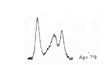
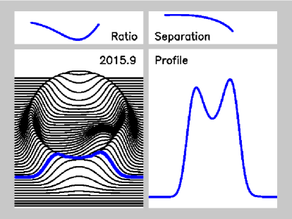
Figure 8: Further evolution of PSR B1913+16’s profile in a simple hollow cone model including an off-centre core component which is visible in the 430-MHz profile (left, Taylor & Weisberg 1982). The right figure is a snapshot of a simulation measuring component amplitude ratio and separation. While the component amplitude ratio first decreases as observed, we can predict that it will rise again as soon as the line-of-sight leaves the core dominated region.

In Fig. 9 we present the latest measurements obtained with the Effelsberg telescope. We also add Weisberg & Taylor’s previously unpublished Arecibo data. As visible from the new measurements, the previously observed trend continues. In the coming years, the decrease in profile width should accelerate drastically, eventually allowing us to turn this qualitative test of general relativity into a quantitative one. For demonstration, we attempted to treat the rate of precession as a free parameter rather than keeping it fixed to the value predicted by general relativity. The result, $\Omega_{p}=1.2\pm 0.2$ deg yr^-1, (shown in Fig. 9) is by no means a precision test and not even a proof of principle! In order to succeed, one has to be confident that the beam structure is modelled correctly. Certainly, this will be the most difficult part of the job. However, it may be possible that an iterative process will be finally successful. Moreover, we did not make much use of the available polarisation information yet. While we used PA data to exclude certain classes of models, we did not invoke RVM fits because of the mentioned large uncertainties. Karastergiou et al. (2000)[49] presented a method where polarisation and pulse shape data can be combined without relying on RVM fits which will become very useful.

Figure 9: Latest results for measurements of the still decreasing component amplitude ratio (left) and the decreasing component separation (right). The left plot contains unpublished data from Jodrell Bank, while the right plots includes previously unpublished data by Weisberg & Taylor (2000). During the fit leading to the results shown on the right, we treated $\Omega_{p}$ as a free parameter.

Combining the polarisation data will be a crucial test, as we should definitely detect changes in the PA swing finally. Eventually, one may obtain reliable measurements of $\Omega_{p}$. However, the most reliable test would be, of course, the re-appearance of the pulsar at about 240 years after it disappears — if we can wait that long.

4 Asymmetric Supernova Explosions

Geodetic precession occurs if the pulsar spin is misaligned with the orbital momentum vector. For PSR B1913+16, we can measure this misalignment angle using the observed precession effects to obtain $\lambda\approx 22^{\circ}$. The question about the origin of this angle is far from trivial. In fact, a non-zero $\lambda$ is the imprint of the violent birth event which created the DNS. It is the ultimate proof that supernova explosions are asymmetric.

4.1 The Birth of a DNS

In the beginning, a DNS starts off as a massive binary system where the more massive companion eventually explodes and becomes a pulsar. The pulsar is probably born with an initial period of 10–30 ms and a high spin-down rate $\dot{P}$ (upper left region in $P-\dot{P}$-diagram, Fig. 10). As the rotation slows down to a period of a few seconds, the pulsar emission eventually ceases after tens of million years or so, moving the pulsar to the lower right corner of the $P-\dot{P}$-diagram. When the massive companion evolves and overflows its Roche-Lobe, the binary system reaches a High-Mass X-Ray Binary phase. The dead pulsar accretes matter and angular momentum. This spin-up “recycles” the pulsar, which re-appears as a millisecond pulsar in the lower left part of the $P-\dot{P}$-diagram. The spin period achieved during the recycling process depends on the duration of the mass transfer. For low-mass systems this phase can be rather long, resulting in periods of a few ms as usually observed for pulsars with white-dwarf companions. In the case of high-mass systems however, this phase is ultimately limited by the event of the supernova explosion (SN) of the companion.

Just prior to the explosion of the companion, the binary system is expected to consist of a recycled pulsar in a circular orbit about its companion, which has evolved to a He-star[50]. All spin vectors are aligned as a result of the angular moment transfer during the accretion process and a following common envelope phase. When the He-star explodes, the pulsar itself is not directly affected by the explosion, since its cross section is too small. In contrast, the survival of the binary system depends on a number of lucky circumstances.

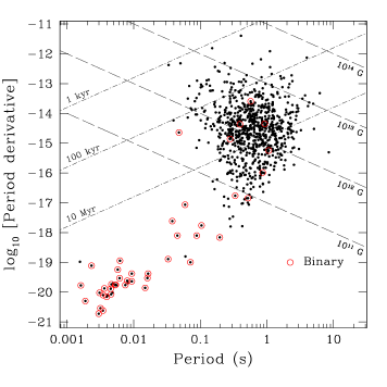
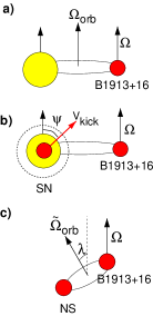
Figure 10: left) $P-\dot{P}$-diagram as known at the time of writing. Binary pulsars are marked with circles. Lines of constant age and surface magnetic field strengths are indicated; right) evolutionary stages of the PSR B1913+16 (a) before and (c) after the second supernova explosion. Before the explosion all spin vectors are aligned. After the explosion, imparting a kick to the companion, the new orbit is misaligned to the previous orbit.

If the explosion is symmetric, the survival will be mainly determined by the total mass loss. Reality, however, is more complicated, since there is convincing evidence that SNe are in fact asymmetric. In that case, a momentum “kick” is imparted to the newly born neutron star. Unless the magnitude and direction of the kick are favorable, the binary system disrupts[50].

4.2 The Kick — Lessons from Geodetic Precession

The actual process causing the kick is still poorly understood. Most of the proposed models, which can be roughly classified as electromagnetic kicks, neutrino driven kicks or hydrodynamical kicks, either produce velocities too small compared to observations, or require unrealistic conditions such as extremely large magnetic fields[51]. It turns out that it is rather difficult to produce kick velocities in excess of, say, 300 km s^-1. In a recent work, Wex et al. (2000) have used the system information obtained by geodetic precession for PSR B1913+16 to derive constraints on the kick mechanism[52].

Since the recycled pulsar is unaffected by the explosion of its companion, its spin vector will continue to point in the direction of the pre-SN orbital angular momentum. The new orbital plane, and hence the new orbital angular momentum, is determined by the direction and magnitude of the kick and will be usually different from the old orbit. As a result, the two vectors are misaligned and gravitationally coupled – geodetic precession occurs(Fig. 10).

Figure 11: Profiles of PSR B1534+12 as measured by Stairs et al. (2000) at 430 MHz (left) and 1400 MHz (right). Changes due to geodetic precession are clearly visible.

It is possible to write down a set of equations relating the pre- and post-SN orbit using conservation of momenta, conditions for the orbit, typical sizes of He-star etc[50]. Knowing that all spin vectors before the SN had been aligned, and assuming that the system velocity after the second SN is dominated by the effects of the kick, we can infer those kick parameters that are necessary to explain the post-SN system characteristics. This procedure is possible for PSR B1913+16 (Wex et al. 2000)[52]: Because of its nature as a DNS, both stars do not interact, but the system’s evolution is solely determined by the emission of gravitational waves and its motion in the galactic potential. Both can be calculated backwards in time. The (justified) assumption that the system was born in the galactic plane, marks the termination point of this backwards computation. The derived orbit and system velocity must then be similar to the conditions just after the SN.

With the unmeasurable radial velocity as the only free parameter, only three different cases are consistent with the age of the pulsar and the system’s current motion away from the plane. Considering all these cases and possible pro- and retro-grade solutions, Wex et al. (2000) reach a number of interesting conclusions among which are: a) on the average, a larger kick is required to explain a retro-grade solution; b) kick velocities between 300 and 1100 km s^-1 are necessary; c) independent of radial velocity and considered cases, the kick imparted to the companion must have been almost perpendicular to the orbital spin. Given the alignment of all pre-SN spins, the kick was also perpendicular to the rotation axis of the exploding star. That has very interesting implications. Firstly, the duration of the kick must have been short compared to the rotational period of the exploding star (otherwise this velocity component would have disappeared). Secondly, if we assume that the magnetic field of the companion was more or less aligned with the rotational axis, as it is the case for the Earth or Sun, the kick was also perpendicular to the magnetic axis. The latter rules out all kick mechanisms which have a preference in the direction of the magnetic field, as for instance some neutrino oscillation models[51].

Yet again, pulsars can obviously serve as diagnostic tools for studying a rather different branch of astrophysics. By carefully investigating this particular binary system, we are able to derive important constraints for any kick mechanism proposed, i.e. every proposed model should be able to produce a short kick perpendicular to the rotation axis.

5 Evidence for Geodetic Precession — Part II.

5.1 Geodetic Precession and PSR B1534+12

The next obvious source to look for evidence of geodetic precession is the second DNS discovered in the disk of our Galaxy, PSR B1534+12[53]. This 38-ms pulsar happens to be brighter than PSR B1913+16, exhibiting also a much narrower pulse peak which both lead to a much better timing accuracy. The fortunate edge-on orientation of the orbit allows the measurement of two PK parameters describing the Shapiro delay of the pulse arrival times. In total five PK parameters can be measured[54] (see Stairs, these proceedings). With the mass estimates of $m_{p}=1.334\pm 0.002$ and $m_{c}=1.344\pm 0.002$ (Table 1), the expected precession rate of $\Omega_{p}=0.51^{\circ}$ yr^-1 is much lower than that of PSR B1913+16 (Fig. 12). Nevertheless, Arzoumanian (1995)[55] and Stairs et al. (2000)[56] succeeded in detecting secular changes in the pulse profiles providing further evidence for geodetic precession acting in binary pulsars (Fig. 11).

The profiles of recycled pulsars with periods less then 50 ms do not seem to fit the classical hollow-cone beam model anymore[57]. This may stem from the extreme compactness of millisecond pulsar magnetospheres, whose sizes scale with the pulse period. The difficulties in modelling the profile changes observed for PSR B1534+12 in a manner done for PSR B1913+13 are hence unfortunate but not too surprising. The situation can possibly be saved by the excellent polarisation data available. Since emission can be seen for almost 80% of the pulse period, RVM fits provide information about the viewing geometry of PSR B1534+12 with an accuracy much better than for most other pulsars[56].

5.2 PSR J1141$-$6545 — Further Evidence?

The latest relativistic binary discovered in the Parkes Multibeam Survey[3], PSR J1141$-$6545, was first considered to be a DNS. The short orbital period of 4.7 hours and an orbital eccentricity of $e=0.171$ (Tab. 1) fit well into the range known for DNSs. Soon after its discovery, the first PK parameter could be measured, i.e. the periastron advance, $\dot{\omega}$. Assuming that its value is completely determined by relativistic effects, general relativity then allows one to determine the total mass of the system[10], $M=m_{p}+m_{c}=2.4$. Assuming a canonical pulsar mass of $m_{p}\approx 1.4$ leaves only $m_{c}\approx 1$ for the companion. These estimates lead to the conclusion that the companion is almost certainly a heavy white dwarf[3].

The exact mass distribution in the system can be determined if a second PK parameter is measured, which should be easily possible in the future. For the moment, we can make use of the mass function of the binary system which indicates that the inclination angle must be close to $i=90^{\circ}$ to produce a pulsar mass of $m_{p}=1.4$. Using these values, the predicted precession rate is the largest for any known system, i.e. $\Omega_{p}\approx 1.35$ deg yr^-1. For smaller (though unlikely) inclinations, the value even increases (see Fig. 12).

Obviously, even as a pulsar-white dwarf system, PSR J1141$-$6545 is a prime candidate to exhibit geodetic precession. It turns out that the same spot of sky had been surveyed at least twice ten years ago, but no pulsar was discovered, neither at 430 nor at 1400 MHz. Today, the pulsar is fairly strong at both frequencies, with a flux density several times that of the detection limit of the previous surveys (Fig. 12). Unless other effects like man-made radio interference are responsible for the previous non-detections, it is conceivable that the pulsar is indeed precessing and has moved its beam into our line-of-sight during the past ten years. If that is the case, future observations should show profile changes soon. Since the pulsar is strong and also polarised, we can hopefully present further detailed evidence for geodetic precession in the near future.

Figure 12: left) Precession rates as predicted by general relativity for the sources discussed here and a further DNS PSR B2127+11C. Unfortunately, its pulsar is rather weak. The precession rate for PSR J1141$-$6545 is given as a function of the unknown orbital inclination angle; right) profiles of PSR J1141$-$6545 at 430 and 1400 MHz (Kaspi et al. 2000).

6 Outlook

It is clear from the presented observational evidence that general relativity correctly predicts the existence of geodetic precession. While the presently available data provide only qualitative tests so far, quantitative tests may be possible if the pulsar emission beam can be modelled sufficiently. Alternatively, polarisation data may produce reliable geometry information via RVM fits, so that a measurement of $\Omega_{p}$ will be possible.

Although the analysis of pulse structure data is the most approachable method to investige geodetic precession, recently Doroshenko et al. (in prep.) investigated the effects on pulsar timing in more detail. It turns out that geodetic precession may produce after all a measurable effect in the timing. Applying their calculations to PSR B1913+16 leads however to the conclusion that this effect may be absorbed in the fits for $P$ and $\dot{P}$, since the pulsar may only be visible for 60 to 80 years. It has yet to be determined as to whether other pulsars could be useful.

As we have seen, one major consequence of geodetic precession can be the (temporary) disappearance of a known pulsar from the sky. Over a time span that is long compared to typical precession periods, i.e. several hundreds to thousands of years, more DNSs will be discovered and measured than without geodetic precession. However, for the typical life time of a scientist, the relevant numbers will not change: the number of binary pulsars that will disappear from the sky before we can detect them should be similar to the number of sources turning up for the first time. In other words, we live in a “steady-state precessing pulsar universe”, so that birth rate and hence detection calculations for gravitational wave detectors are unaffected by the discussed phenomena. While this consideration certainly applies in general, it is a very reasonable idea to occasionally re-search the position of known DNSs with large precession rates to check for the appearance of previously unseen companions. You never know…

References

- [1] A. Hewish, et al, Nature 217, 709 (1968).
- [2] R.A. Hulse and J.H. Taylor, Astrophys. J. 195, L51 (1975).
- [3] V.M. Kaspi, et al., Astrophys. J. 543, 321 (2000).
- [4] R.T. Edwards and M. Bailes, Astrophys. J., astro-ph/0010599 (2001).
- [5] F. Camilo, et al., Astrophys. J. submitted, (2001).
- [6] J.F. Bell and T. Damour, Class. Quantum Grav. 13, 3121 (1996).
- [7] C. Lange, et al., Mon. Not. R. astr. Soc. submitted, (2001).
- [8] N. Wex, ASP Conf. Ser. 202, 113 (2000).
- [9] A.G. Lyne, et al., Mon. Not. R. astr. Soc. 312, 698 (2000).
- [10] T. Damour and J.H. Taylor, \Journal\PRD4518401992.
- [11] D.C. Backer and R.W. Hellings, Ann. Rev. Astr. Ap. 24, 537 (1986).
- [12] T. Damour and R. Ruffini, Academie des Sciences Paris Comptes Rendus Ser. Scie. Math., 279, (1974).
- [13] S.E. Thorsett and D. Chakrabarty, Astrophys. J. 512, 288 (1999).
- [14] J.R. Oppenheimer, G. Volkoff, Phys. Rev. 55, 374 (1939).
- [15] G.G. Pavlov and V.E. Zavlin, Astrophys. J.L̇ett. 490, L91 (1997).
- [16] K. Brecher and M.P. Ulmer, Nature 271, 135 (1978).
- [17] M. Kramer, et al., Astr. Astrophys. 306, 867 (1996).
- [18] M. Blaskiewicz, PhD thesis, Cornell University (1991).
- [19] D.C. Backer, Nature 228, 42 (1970).
- [20] A.G. Lyne, Mon. Not. R. astr. Soc. 153, 27 (1971).
- [21] M. Kramer, et al., Astrophys. J. 520, 324 (1999).
- [22] M.M. Komesaroff, Nature 225, 612 (1970).
- [23] L. Oster and W. Sieber, Astrophys. J. 203, 233 (1976).
- [24] J.M. Rankin, Astrophys. J. 274, 333 (1983).
- [25] M. Kramer, et al. Astr. Astrophys. Suppl. 107, 515 (1994).
- [26] K.M. Xilouris, et al., Astr. Astrophys. 309, 481 (1996).
- [27] V. Radhakrishnan and D.J. Cooke, Astrophys. Lett. 3, 225 (1969).
- [28] B.M. Barker and R.F. O’Connell, Astrophys. J. Lett. 199, L25 (1975).
- [29] B.M. Barker and R.F. O’Connell, \Journal\PRD123291975.
- [30] L.W. Esposito and E.R Harrison, Astrophys. J. Lett. 196, L1 (1975).
- [31] G. Boerner, et al, Astr. Astrophys. 44, 417 (1975).
- [32] J.H. Taylor and J.M. Weisberg, Astrophys. J. 345, 434 (1989).
- [33] T. Damour and J.H. Taylor, Astrophys. J. 366, 501 (1991).
- [34] J.H. Taylor, Les Prix Nobel, Norstedts Tryckeri, Stockholm, 80 (1994).
- [35] J.M. Weisberg, et al, Astrophys. J. 347, 1030 (1989).
- [36] A.G. Lyne and R.N. Manchester, Mon. Not. R. astr. Soc. 234, 477 (1988).
- [37] J.M. Cordes, et al., Astrophys. J. 349, 546 (1990).
- [38] J.H. Taylor and J.M. Weisberg, Astrophys. J. 253, 908 (1982).
- [39] A. Wolszczan, et al., Astrophys. J. 528, 907 (2000).
- [40] M. Kramer, Astrophys. J. 509, 856 (1998).
- [41] J.A. Gil, et al, Astr. Astrophys. 132, 312 (1984).
- [42] M. Blaskiewicz, et al, Astrophys. J. 370, 643 (1991).
- [43] M. Bailes, Astr. Astrophys. 202, 109 (1988).
- [44] Y.N. Istomin, Soviet Astronomy Letters 17, 301 (1991).
- [45] J.M. Weisberg and J.H. Taylor, ASP Conf. Ser. 202, 127 (2000).
- [46] J.H. Taylor, Proceedings of the XXXIV’th Rencontres de Moriond, (1999).
- [47] J.H. Taylor, et al., Nature 277, 437 (1979).
- [48] J.H. Taylor and J.M. Weisberg, Astrophys. J. 253, 908 (1982).
- [49] A. Karastergiou, et al., ASP Conf. Ser. 202, 125 (2000).
- [50] C. Fryer and V. Kalogera, V., Astrophys. J. 489, 244 (1997).
- [51] D. Lai, Stellar Astrophysics, astro-ph/9912522 (1999).
- [52] N. Wex, et al, Astrophys. J. 528, 401 (2000).
- [53] A. Wolszczan, Nature 350, 688 (1991).
- [54] I.H. Stairs, et al., Astrophys. J. 505, 352 (1998).
- [55] Z. Arzoumanian, PhD thesis, Princeton University (1995).
- [56] I.H. Stairs, et al., ASP Conf. Ser. 202, 121 (2000).
- [57] M. Kramer, et al., Astrophys. J. 526, 324 (1999).