Formation of massive stars by growing accretion rate

We perform calculations of pre-main sequence evolution of stars from $1$ to $85\,M_{\odot}$ with growing accretion rates $\dot{M}$. The values of $\dot{M}$ are taken equal to a constant fraction $\tilde{f}$ of the rates of the mass outflows observed by Churchwell (church (1998)) and Henning (henning2000 (2000)). The evolution of the various stellar parameters is given, as well as the evolution of the disc luminosity; electronic tables are provided as a supplement to the articles. Typically, the duration of the accretion phase of massive stars is $\simeq 3\cdot 10^{5}\,\mathrm{yr}$. and there is less than $10\%$ difference in the time necessary to form a $8$ or $80\,M_{\odot}$ star. If in a young cluster all the proto–stellar cores start to accrete at the same time, we then have a relation $M(t)$ between the masses of the new stars and the time $t$ of their appearance. Since we also know the distribution of stellar masses at the end of star formation (IMF), we can derive the star formation history $N(t)$. Interestingly enough, the current IMF implies two peaks of star formation: low mass stars form first and high mass star form later.

1 Introduction

Two scenarios have been proposed to explain the formation of massive stars. Star coalescence (Bonnell et al. bonnell (1998); Stahler et al. stahler (1998)) and the accretion scenario (Beech & Mitalas beemit (1994); Bernasconi & Maeder bermae (1996)). The merging of stars requires very high stellar densities ($\geq 10^{4}\,\mathrm{stars}\,{\mathrm{pc}^{-3}}$) to be efficient (Bonnell et al. bonnell (1998); Henning henning (2001)).

The imaging of new-born stars with the HST (Burrows et al. burrows (1996)), the IRAM interferometer (Dutrey dutrey (1998)), the VLA (Wilner & Ho & Kastner & Rodríguez wilneretal (2000)) and the VLT (Brandner brandner (2000)), among others) clearly shows discs (or remnants of discs), favouring the accretion scenario for low and intermediate mass stars. The jets and/or outflows that are sometime observed are closely related to accretion discs; they can contribute to solve the angular momentum problem (Tomisaka tomisaka2 (2000)).

Accretion rates of the order of $10^{-5}$ to $10^{-4}\,M_{\sun}\,\mathrm{yr}^{-1}$ explain very well low mass stars (Palla palla (1998)). But such values fail to describe the formation of massive stars, because with such rates the massive stars would leave the ZAMS (i.e. would have burned a significant part of their hydrogen) before being fully formed, as pointed out by Nakano (nakaal3 (1988)) and Norberg & Maeder (normae (2000)). Nakano (nakaal2 (2000)) studied the implications of a huge constant accretion rate of $\approx 10^{-2}\,M_{\sun}\,\mathrm{yr}^{-1}$ for an observed $10^{5}\,L_{\sun}$ protostar.

The reality could well lie between these two models. Can an accretion rate that depends on the stellar mass (or luminosity) describe the star formation from low to very high masses ? This is the question of the growing accretion rates.

A nice observational relation between the outflow mass rates and the stellar bolometric luminosities in ultra compact ${H\textsc{ii}}$ regions was established by Churchwell (church (1998)) over the ranges $1$ to $10^{6}\,L_{\sun}$ and $10^{-6}$ to $10^{-2}\,M_{\sun}\,\mathrm{yr}^{-1}$. Independent observations by Henning et al. (henning2000 (2000)) confirm its validity.

Churchwell’s relation can bring some new constraints for the scenarios of the formation of massive stars. A crucial question is to know if the accretion scenario is compatible or not with this relation. The relation can bring something new to the description of the pre-main sequence evolution of stars and for the explanation of the rapid birth of massive stars. The relation can also be a used as a strong check for the computer simulations of discs around stars and the jets/outflows, and offers the possibility to fix uncertain parameters of these models (e.g. viscosity).

The principal properties of stars with accretion discs on the birthline are discussed. Tracks for stars leaving the birthline are calculated. Links between the IMF and the processes that end the stellar mass evolution are also presented.

2 The simulations

Figure 1: The $\log T_{\mathrm{eff}}$ – $\log L$ diagram showing birthlines for 3 values of $\tilde{f}$ and for the model of N&M. The ZAMS is taken from Schaller et al. (schall (1992)). Observations of protostars from the compilation by N&M are shown with discs (respectively circles) if $\dot{M}$ is more (respectively less) than $10^{-5}\,M_{\sun}\,\mathrm{yr}^{-1}$; triangles mean unspecified rates.

The matter which escapes from the disc (in the central region) is divided in two major flows: one part falls on the star while the other part is ejected in the form of jets and outflows. Let us denote by $\dot{M}_{\mathrm{disc}}$ the mass rate transferred inwards from the disc, by $\dot{M}$ the mass rate accreted by the star, and by $\dot{M}_{\mathrm{out}}$ the mass rate in the jets/outflow.

The relation, found by Churchwell (church (1998)) and confirmed by Henning et al. (henning2000 (2000)), between the bolometric luminosity $L$ of stars and the outflow mass rate $\dot{M}_{\mathrm{out}}$ is single valued (at least in the error bars), monotonously increasing and valid over a very wide range of luminosity: from $1$ to $10^{6}\,L_{\sun}$. A polynomial fit of the observations by Churchwell (church (1998)) gives

$$\log{{\dot{M}_{\mathrm{out}}}\over{M_{\sun}\,\mathrm{yr}^{-1}}}=-5.28+\log{L\over{L_{\sun}}}\cdot(0.752-0.0278\log{L\over{L_{\sun}}}).$$

Unfortunately, there is at present no similar relation available between $L$ and $\dot{M}$; one must parameterize the ratio between the accretion and outflow fluxes and do some suppositions about their proportion before being able to model the evolution of the central star. Let be $\dot{M}=\tilde{f}\,\dot{M}_{\mathrm{out}}$, $\dot{M}=f\,\dot{M}_{\mathrm{disc}}$ and $\dot{M}_{\mathrm{out}}=(1-f)\,\dot{M}_{\mathrm{disc}}$ so that $\tilde{f}=f/(1-f)$. A variety of physical parameters could have effects on $\tilde{f}$ (or $f$): chemical compositions, metallicities, magnetic fields, rotational velocity of the star. Some other parameters have certainly a role to play, but are not yet firmly defined, like the dust opacity. Therefore, obtaining a theoretical value of $f$ is very difficult. Nonetheless, Tomisaka (tomisaka1 (1998)) found $f\approx 1/3$ with his numerical MHD-simulation of a low mass class $0$ protostar. Shu et al. (shuetal (1998)) deduced a similar value with their model of X-wind magnetic configuration, also for a low mass star. From his measurements of the far-infrared luminosity of a B star and the mass of its outflows, Churchwell (church (1998)) estimated a slightly smaller value, of the order of $f\approx 0.15$.

Due to the great number of changing physical parameters which can have an effect on $f$, $f$ is probably non-constant during the evolution of accreting stars. The last three values of $f$ cited above suggest that $f$ could be a decreasing function of the stellar mass, but this is far from being firmly established. For this preliminary study, we simplify this huge astrophysical problem, retaining only a ratio $f$ that is constant during the whole accretion period.

The ”best” $f$ is presently unknown. A way to assign a more or less realistic value to $f$ is as follows. The birthline is the path in the HR diagram that continuously accreting stars follow. Stars on the birthline are difficult to observe, because they are hidden by the accretion disc and a dense cocoon of interstellar matter. The star becomes visible once a sufficient amount of the surrounding matter has been dispersed. It follows that the young stars are observed generally between the birthline and the zero age main-sequence (ZAMS). Before hydrogen ignition, gravitational contraction and deuterium burning are the main energy sources for the star; the localization of the birthline depends on the deuterium accretion rate. We will choose $\tilde{f}$ as the value for which the computed birthline fits ”at the best” the upper envelope of the observations of young stars in the pre-main sequence part of the HR diagram (as in Norberg & Maeder normae (2000), denoted hereafter N&M).

The evolution of the pre-main sequence models with growing accretion rate is computed with the Geneva code (Meynet & Maeder meymae (2000)), under the assumption of a non-rotating star, at $Z=0.02$ and at deuterium concentration $5\cdot 10^{-5}$. Winds are not taken into account.

The computations begin with a fully convective $0.7\,M_{\sun}$ protostar which is taken to be $7\cdot 10^{5}\,\mathrm{yr}$ old, in agreement with models of low mass star formation (Palla palla (1998)). The mass of the protostar grows at a rate $\dot{M}=\max(10^{-5}\,M_{\sun}\,\mathrm{yr}^{-1},\,\tilde{f}\,\dot{M}_{\mathrm{out}})$.

We compare the models with accretion rates parameterized by the bolometric luminosity of the star to the model of mass parameterized accretion rate found by N&M: $\dot{M}=10^{-5}\cdot\max(1,\,M)^{1.5}$ where units are $M_{\sun}$ and $M_{\sun}\,\mathrm{yr}^{-1}$. The $M$- and $L$-parameterized accretion rates are different in the sense that the first one depends only on one parameter (the mass) of the star, and the second one depends on many involved quantities (mass, profiles of chemical composition and internal energy, etc.) and thus is sensitive to the history of the star (e.g. opacity via chemical abundances, diffusive processes). For this reason, the memory of the initial luminosity of the star in the $M$-parameterization is rapidly lost. This is not the case for the $L$-parameterized accretion; if the initial star is over-/under-luminous, the luminosity of the accreted deuterium is also above/below the normal value and the birthline is also over-/under-luminous. This sensitivity to the initial conditions for the $L$-parameterized accretion remains small with respect to the possible variations of the birthlines with $f$, for stars initially on the Hayashi band. Processes that depend on their past can ”easily” oscillate or even be chaotic, for physical reasons (Hairer et al. haireral (1987)) or for numerical reasons (Bergé et al. bergal (1988)). Apparently the calculations do not reveal strong signatures of instabilities, except maybe some oscillations near the surface of accreting stars above $22\,M_{\sun}$.

3 Results and discussions

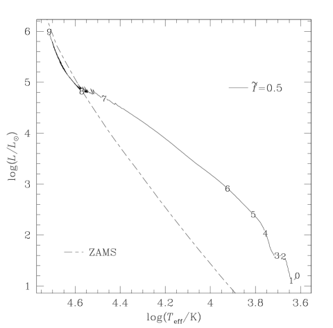
Figure 2: A birthline in $\log T_{\mathrm{eff}}$ – $\log L$. Some key phases are highlighted: $0$: initial conditions - $1$: central ignition of deuterium - $2$: central gravitation dominates over ${{}^{2}H\textsc{}}$-burning - $3$: start of shell deuterium-burning - $4$: end of large scale convection - $5$: end of thin central convection - $6$: central ${{}^{2}H\textsc{}}$-exhaustion - $7$: central ignition of hydrogen and restart of core convection - $8$: arrival on the ZAMS - $9$: star starts evolving away from the ZAMS.

The first step consists of the estimate of a plausible $\tilde{f}$. The second step is the prediction of physical parameters for the stars and discs using the $\tilde{f}$ found. Connections with the IMF is postponed to the next section.

Before hydrogen ignition, the main energy sources for the star are gravitational contraction and deuterium burning. The localization of the birthline is then governed essentially by the deuterium accretion rate on the star. The higher $\dot{M}$, the higher the birthline in the HR diagram.

Table 1: Properties of stars on the birthline with $\tilde{f}=0.5$: age, luminosity, mass, effective temperature, radius, relative upper radius of the convective zone. The ratio of disc and star luminosities is also given.

$\begin{array}[]{ccccccc}t/\mathrm{yr}&L/L_{\sun}&M/M_{\sun}&T_{\mathrm{eff}}/\mathrm{K}&R/R_{\sun}&R_{\mathrm{conv}}^{\mathrm{sup}}/R&L_{\mathrm{disc}}/L\\[2.84526pt] 70.01e3&16.00&0.700&4110&7.88&1.000&4.17\\ 74.50e3&15.14&0.785&4176&7.43&1.000&6.22\\ 81.20e3&13.24&0.901&4290&6.58&1.000&8.33\\ 88.45e3&12.82&1.02&4377&6.22&1.000&9.80\\ 98.13e3&15.41&1.19&4442&6.63&1.000&9.75\\ 114.5e3&23.30&1.55&4533&7.82&1.000&9.47\\ 130.1e3&33.25&1.99&4639&8.92&1.000&9.67\\ 159.0e3&38.91&2.98&4890&8.68&1.000&14.6\\ 188.2e3&38.91&3.99&5112&7.95&1.000&21.4\\ 217.0e3&48.80&5.05&5358&8.10&1.000&24.0\\ 232.8e3&379.1&6.01&7036&13.1&0.000&8.32\\ 239.8e3&2.662e3&8.05&11.73e3&12.5&0.000&5.21\\ 242.8e3&9.100e3&10.0&16.55e3&11.6&0.000&4.00\\ 244.6e3&21.58e3&12.0&21.79e3&10.3&0.000&3.55\\ 246.2e3&46.77e3&15.0&29.76e3&8.13&0.001&3.92\\ 248.3e3&81.19e3&20.1&37.74e3&6.66&0.135&5.17\\ 250.2e3&87.63e3&25.0&39.40e3&6.35&0.229&6.65\\ 251.9e3&132.1e3&30.0&42.61e3&6.66&0.234&5.50\\ 254.5e3&256.7e3&40.0&46.59e3&7.77&0.265&4.85\\ 256.4e3&372.3e3&49.9&48.17e3&8.75&0.272&3.82\\ 258.1e3&495.1e3&59.7&49.37e3&9.61&0.288&3.73\\ 259.7e3&680.4e3&70.6&50.70e3&10.7&0.299&3.31\\ 260.9e3&825.5e3&79.4&51.49e3&11.4&0.305&3.02\\ 261.6e3&952.7e3&84.9&51.84e3&12.0&0.312&2.87\par\end{array}$

Figure 1 shows birthlines for different values of $\tilde{f}$, and the observations compiled in N&M. While $\tilde{f}=0.3$ seems to be a little too low, $\tilde{f}\in\{0.4,\,0.5\}$ give reasonable envelopes to the observations. Two statistical biases in the estimate of the envelope are possible, with consequences for the determination of $\tilde{f}$. 1) The stars which constrain the birthline are usually all on one side of the birthline (a nonsignificant exception is nevertheless visible in Fig. 8). Because the density of stars near the birthline is small, the probability that one misses a crucial observation is relatively large. The effect of this bias is an underestimated luminosity of the envelope of the observation and thus also of the birthline. Unfortunately, this occurs in the upper pre-main sequence part of the HR diagram where the sensibility of the computed birthline to $\tilde{f}$ is the greatest. The deficiency of stars in this region is due to the very short time spent by a star in this region, as will be shown in Fig. 8. 2) The stars leave the birthline faster than they reach the ZAMS. In other words, the median of the positions of the stars for which the error bars constrain the birthline (by their envelope) is shifted towards the ZAMS; this effect vanishes as error bars go to zero. With these two facts in mind, our preference is for the highest value: $\tilde{f}=0.5$, i.e. $f=1/3$.

The ratio $f=\dot{M}_{\mathrm{out}}/\dot{M}_{\mathrm{disc}}$ supported by Fig. 1 is in good agreement with theoretical estimates of $f\cong 1/3$, as mentioned above.

Properties of stars on the birthline and the relative luminosity of the disc to that of the star, for $\tilde{f}=0.5$, are summarized in Table 1, while Fig. 2 locates different phases of the star evolution in the HR diagram.

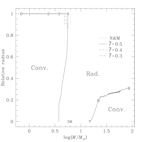
Figure 3: Location of the convective and radiative zones. The relative radius of the boundaries between the convective and radiative zones are drawn for the birthline with $\tilde{f}=0.5$. For the other birthlines, only the beginning of the fully radiative state is shown. The small labels denote the evolutionary stages shown in Fig. 3.

The ${{}^{2}H\textsc{}}$-burning begins at the center of the star. Nascent stars of mass below $3.8\,M_{\sun}$ ($\log(M/M_{\sun})=0.58$) are fully convective (Fig. 3), and the deuterium accreted is carried inside the star where it is burnt. As the temperature rises, the deuterium burns farther from the center. At $3.8\,M_{\sun}$, a radiative core is created, and the accreted deuterium is then burnt in a shell at the periphery of this core; the star inflates (second hump in Fig. 4) and the luminosity grows. If the relation of the $L$-parameterized accretion is right, and in particular its single valued character, the shell ${{}^{2}H\textsc{}}$-burning could play a major role in the beginning of star formation, raising the stellar luminosity and inducing via Churchwell’s relation, a real boost in the accretion rate, shortening the time needed to reach high mass stars. The convective ${{}^{2}H\textsc{}}$-burning shell becomes thin at the surface of the star around $5.6\,M_{\sun}$ ($\log(M/M_{\sun})=0.75$) (slightly depending on the mass accretion rate); the star becomes fully radiative.

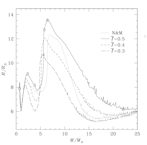
Figure 4: $M$ – $R$ relation for stars evolving on the birthlines.

The luminosity of the ${{}^{2}H\textsc{}}$-burning is governed by the accretion rate; the star inflates to balance a excess of power, or contracts during a shortage of deuterium. The $R(M)$ relation (Fig. 4) is thus very sensitive to $\dot{M}$ during the pre-main sequence evolution of the star and especially during the fully radiative phase.

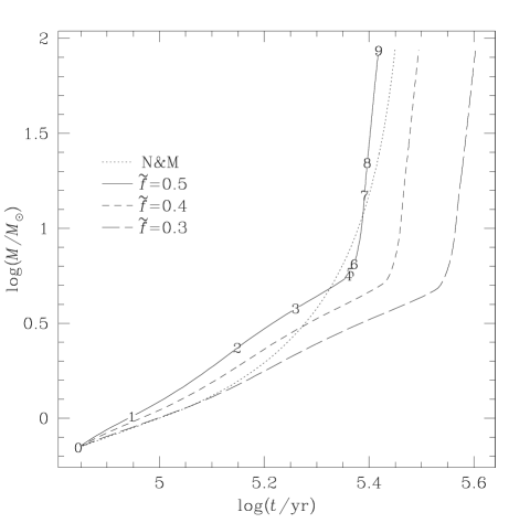
Figure 5: Mass evolution for stars on the birthlines.

The consequences of the luminosity’s growth during the shell ${{}^{2}H\textsc{}}$-burning are clearly visible in the $\log t$ – $\log M$ diagram (Fig. 5) in the form of an elbow near $\log(M/M_{\sun})=0.8$ ($6\,M_{\sun}$) with a rather abrupt change of slope in the curves, for the $L$-parameterized accretion. Below the bend, the much smoother curve of the $M$-parameterized accretion of N&M is a little bit higher than the one for the $L$-parameterized accretion, and lower afterwards. Rather than physical, the origin of this difference resides in the choice of the parameterization for $\dot{M}$. Because both laws were adjusted on the same observations, they globally look alike and make similar predictions, but they can locally differ.

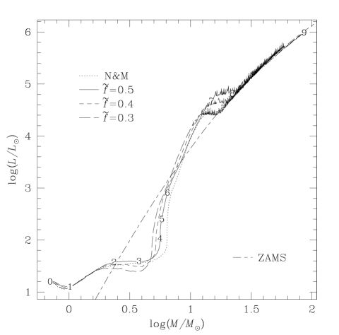
Figure 6: $\log M$ – $\log L$ relation of stars on the birthlines.

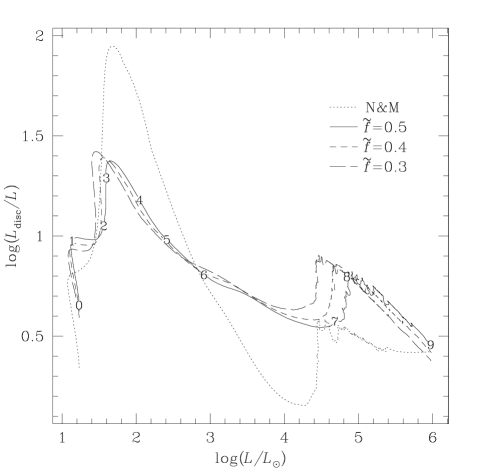
Figure 7: Relative luminosity of disc to that of the star as a function of stellar bolometric luminosity for stars evolving on the birthlines. For the model of N&M, $\tilde{f}=0.5$ is assumed.

Figure 8: Tracks in $\log T_{\mathrm{eff}}$ – $\log L$ followed by stars that leave the birthline with $\tilde{f}=0.5$. Couples of numbers represent the age $t_{\mathrm{stop}}$ of the star (in units of $10^{3}\,\mathrm{yr}$) at the stop of the accretion, and its mass (in $M_{\sun}$) on the ZAMS. For the stars which are no longer on the birthline, the small dots at $\log T_{\mathrm{eff}}\approx 3.75$ correspond to the beginning of the fully radiative interiors; the small dots close to the ZAMS correspond to the appearance of the convective cores.

One half of the gravitational energy gained during the rotational infall is transformed into kinetic energy; the other half is used to heat up the disc and is eventually radiated. Chemical energies (sublimation of dust and grains, ionization) are small with regards to gravitational energy and are neglected in the computations. The disc luminosity, $L_{\mathrm{disc}}$, is thus of the order of $G\,M\,\dot{M}_{disc}\,/\,(2\,R)$, as given by Hartmann (1998a , §5.4). It appears in Fig. 7 that during the accretion phase, the luminosity of the disc is always greater than the star luminosity. On the birthline, the star encounters three phases of nearly constant luminosity. In these phases, the radius of the star shrinks while the mass continues to grow; according to the previous formula, the luminosity of the disc grows. That explains the three vertical steps in the $\log L$ – $\log(L/L_{\mathrm{disc}})$ diagram. The step around $\log(L/L_{\sun})=4.8$ corresponds to the arrival of the star on the ZAMS and is the only feature really sensitive to $\tilde{f}$. The probability of having good observations of stars in this region of the diagram is very small and we conclude that the relative luminosity of the disc to that of the star cannot help us to fix $\tilde{f}$. The smaller variability of the ratio of disc to star luminosities for the $L$-parameterized accretion than for the $M$-parameterized accretion has the same origin as in the $\log t$ – $\log M$ diagram.

After the accreting star has joined the ZAMS, at $22\,M_{\sun}$, it evolves in a very similar manner to the one calculated in N&M. They used $\dot{M}\propto M^{1.5}$ and the linear fit in Churchwell’s data implies $\dot{M}\propto M^{1.54}$ using the $L(M)$ relation on the ZAMS. An accretion rate of $8\cdot 10^{-3}\,M_{\sun}\,\mathrm{yr}^{-1}$ is obtained for a $85\,M_{\sun}$ star. Though it seems very high, this rate is still in the permitted domain of accretion with spherical symmetry (Wolfire & Cassinelli wolcas (1987)); if the accretion is made via a disc, even higher rates are permitted due to the less important cross-section of infalling material to radiations from the star and from the shock, and to the enhanced cooling (Nakano nakaal3 (1988); Henning henning (2001)).

Once the disc is no longer fed by its environment, for example by the disappearance of the parent cloud by the outflows of the star or jets/ouflows and the radiation of neighbouring hot luminous stars (Nakano et al. nakaal1 (1995)), the disc get thinner by accretion and evaporation. The transition from active to passive discs is probably a smooth function of time. As its mass decreases, the residual disc plays a smaller and smaller role in the evolution of the star. Both the mass of discs and the typical duration of the transition are still very uncertain; in the computations, we neglect their effects, using an instantaneous stopping of the accretion at time $t_{\mathrm{stop}}$. Figure 8 shows the resulting theoretical tracks for some values of $t_{\mathrm{stop}}$ (in units of $10^{3}\,\mathrm{yr}$).

The following considerations can partly justify the assumption that from a certain stage, the disc has no more significant influence on the central star. For low and intermediate mass stars, the disc is usually lighter than the central star (Hartmann 1998a , §§6.3 and 9.7, 1998b ; Bernasconi bernasconi (1997)). Observations of the residual mass transfer rate of the disc around T Tauri stars is described by Hartmann (1998b ); they can be approximately represented by $\log\dot{M}_{\mathrm{disc}}^{\mathrm{res}}\approx 0.4-1.4\,\log\tilde{t}$ (units are $M_{\sun}\,\mathrm{yr}^{-1}$ and $\mathrm{yr}$), where $\tilde{t}$ is a relative scale for the ages. Integrating $\dot{M}_{\mathrm{disc}}^{\mathrm{res}}$ from the $\tilde{t}$ corresponding to a disc mass transfer rate $(1+\tilde{f})\,\dot{M}_{\mathrm{out}}$ at $t_{\mathrm{stop}}$ to infinity, one finds a crude estimate of the mass of the disc at the moment of the stopping of the accretion: $M_{\mathrm{disc}}\approx 5\,\dot{M}_{\mathrm{disc}}{}^{0.3}$ (units are $M_{\sun}$ and $M_{\sun}\,\mathrm{yr}^{-1}$). $\dot{M}_{\mathrm{disc}}$ is probably out of the validity domain for $\dot{M}_{\mathrm{disc}}^{\mathrm{res}}$, but $f\,M_{\mathrm{disc}}$ remains less than $5\%$ of the mass of the star, for $M>2\,M_{\sun}$. Bernasconi (bernasconi (1997)) studied the residual mass accretion of dying discs, but his models contain many arbitrary parameters; for intermediate mass stars, the difference between the tracks with and without residual accretion are nonetheless much smaller than the error bars of the present day observations.

The time $t_{\mathrm{stop}}$ corresponds approximately to the time at which the cocoon of interstellar matter vanishes, thus the star becomes visible in the optical bands only after this moment; the location of the first optical visibility of stars above $22\,M_{\sun}$ is very close to the ZAMS.

For the stars studied in this paper (mass on the ZAMS $>1.19\,M_{\sun}$), there are four regions in the pre-main sequence part of the HR diagram, as shown in Fig. 8. 1) For $\log T_{\mathrm{eff}}$ below $\approx 3.68$ (i.e. $4.8\cdot 10^{3}\,\mathrm{K}$), the stars are fully convective; they leave the birthline with a vertical Hayashi-like displacement in the HR diagram. No more accreting stars between $\log T_{\mathrm{eff}}\approx 3.68$ and $\log T_{\mathrm{eff}}\approx 3.76$ (i.e. $5.8\cdot 10^{3}\,\mathrm{K}$) have a radiative core surrounded by a convective ${{}^{2}H\textsc{}}$-burning shell; if the star already has a radiative core before the end of accretion, the track closely follows the birthline (with an increasing luminosity) for a short period of time after $t_{\mathrm{stop}}$; if a radiative core is absent, one is swiftly created after the end of accretion and the star leaves the birthline with a decreasing luminosity. 3) For $\log T_{\mathrm{eff}}$ above $\approx 3.76$, the stars are fully radiative, except on 4) a small band above the ZAMS where stars already have a convective ${H\textsc{}}$-burning core.

Electronic tables for the tracks are available via the anonymous ftp server of the Geneva observatory; the file is located in directory
$ftp://obsftp.unige.ch/pub/evol/prems/AA2001BM$ .

4 Relation with the IMF

The initial mass function (IMF) represents the density of probability that a star ends its accretion with a given mass. The IMF results from many physical phenomena (fragmentation of the parent cloud, vanishing of the reservoir of interstellar matter, accretion rate and its efficiency, binarity, etc.). But under the assumption that the accretion rate does not depend on the local conditions of the cloud and disc, the IMF can be seen as the result of the mechanisms that end the feeding of the disc with interstellar matter (in the case of a small ratio of disc to star masses).

The IMF is usually noted $\xi(m)$. $\xi(m)\,\mathrm{d}m$ is the relative number of new-born stars in the mass interval $\mathrm{d}m$ centered on $m$; the IMF is normalized so that $\int_{M_{\min}}^{M_{\max}}\,\xi(m)\,\mathrm{d}m=1$. The assumptions made for the models of this paper imply that the star mass evolution on the birthline is a single valued and monotonously increasing function $M(t)$. Thus, from the observed IMF and using the $M(t)$ relation (as in Fig. 4), one can compute the density of probability $P(t_{\mathrm{stop}})$ of the age $t_{\mathrm{stop}}$ of stars when the accretion is abruptly stopped:

$$P(t_{\mathrm{stop}})=(\xi(M(t))\,\mathrm{d}M(t)/\mathrm{d}t)|_{t=t_{\mathrm{stop}}}.$$

The result is shown in Fig. 9, using the IMF of Kroupa (kroupa (2001)): $\xi(m)=\beta\,m^{-\alpha}$ where

$$\left(\alpha;\,\beta\right)=\left\{\begin{array}[]{cl}\left(0.30;\,1.99\right),&$if $m\in[M_{\min}=0.01,\,0.08),\\ \left(1.30;\,0.159\right),&$if $m\in[0.08,\,0.50),\\ \left(2.30;\,0.0795\right),&$if $m\in[0.50,\,M_{\max}=100.]\end{array}\right.$$

The IMF of Scalo (scalo (1998)) differs from Kroupa’s one principally in the $<0.1\,M_{\sun}$ region; both IMFs give similar results.

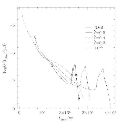
Figure 9: Density of probability of $t_{\mathrm{stop}}$ for mass accretion rates with three values of $\tilde{f}$, and the N&M one. For $t_{\mathrm{stop}}<7\cdot 10^{4}\,\mathrm{yr}$ ($M<0.7\,M_{\sun}$), an accretion rate of $10^{-5}\,M_{\sun}\,\mathrm{yr}^{-1}$ is assumed.

For the $L$-parameterized accretion, the break in the mass evolution graph located near $6\,M_{\sun}$ is great enough to generate a sharp hump (an order of magnitude) in the density of probability of $t_{\mathrm{stop}}$, $P(t_{\mathrm{stop}})$. For the $M$-parameterized accretion of N&M which gives a monotonously decreasing $P(t_{\mathrm{stop}})$, a bump is also distinguishable, but it is smoothed by the nature of the law used. In comparison to the $L$-parameterized accretion rate, the $M$-parameterized accretion rate is indeed a little higher for masses in the range $1.6$ to $6\,M_{\sun}$ and lower for the other stars (Fig. 5). The presence of the peak for the $L$-parameterized accretion does not depend on the ratio $\tilde{f}=\dot{M}/{\dot{M}_{\mathrm{out}}}$ of accreted and ejected masses, if this quantity does not evolve with the mass and luminosity of the star. If theses peaks are confirmed, it would be most interesting to investigate the various physical processes at their origin. One possible way to explain theses curves could be as follows. For stars below $6\,M_{\sun}$, the fractal parent cloud is probably dissipated mostly by neighbouring stars. For stars above $6\,M_{\sun}$, the star and disc luminosities could grow high enough to scatter the parent cloud.

5 Conclusions

Numerical experiments have been done with mass accretion rates proportional to the luminosity parameterized outflow rate

$$\log{{\dot{M}_{\mathrm{out}}}\over{M_{\sun}\,\mathrm{yr}^{-1}}}=-5.28+\log{L\over{L_{\sun}}}\cdot(0.752-0.0278\log{L\over{L_{\sun}}})$$

established by Churchwell (church (1998)) and confirmed by Henning et al. (henning2000 (2000)). Until complete theoretical values of the ratio of accreted on the star and ejected masses, $\tilde{f}=\dot{M}/\dot{M}_{\mathrm{out}}$, are computed taking into account stellar rotation and magnetic field, chemistry, radiative transfers, etc., $\tilde{f}$ can be seen as a unknown parameter.

1. The comparison of theoretical birthlines from different $\tilde{f}$ to observations of young star constraints $\tilde{f}$. For these experiments, we chose constant values for $\tilde{f}$ and our favorite choice is $\tilde{f}=0.5$. This value permits a reasonable fit of the observations of accreting stars.

2. Only a fraction $f=\tilde{f}/(1+\tilde{f})=1/3$ of the mass transferred from the disc in the central region accretes on the star. This ratio is in relative agreement with numerical predictions by Tomisaka (tomisaka1 (1998)) ($1/3$) and the theoretical model of Shu et al. (shuetal (1998)) (also $1/3$), both cases are for low mass stars. Observations by Churchwell (church (1998)) suggest a smaller value (of the order of $0.15$) for a B star; this is not seen as a strong disagreement.

3. The relative lack of observations in the upper pre-main sequence part of the HR diagram is due to the very fast evolution of the stars just before ${{}^{1}H\textsc{}}$-ignition and their arrival on the ZAMS; there are few chances to better constrain $\tilde{f}$ using the HR diagram. Apparently, the ratio of disc to star luminosities cannot help to fix $\tilde{f}$.

4. The $R(M)$ relation is very sensitive to the mass accretion rate during the ${{}^{2}H\textsc{}}$-burning; the biggest differences are located in the range of $7$ to $15\,M_{\sun}$, i.e. when the star is fully radiative and the ${{}^{2}H\textsc{}}$ burns near the surface; for a given mass, the greater the rate, the bigger the radius.

5. The $M$-parameterized accretion rate of Norberg & Maeder (normae (2000)) gives essentially the same birthline in the HR diagram as the $L$-parameterized accretion. The mass evolution of stars with accretion rate parameterized by $M$ is smooth in $\log t$ – $\log M$; on the contrary, the evolution for the mass with the $L$-parameterized accretion shows a sharp transition near $6\,M_{\sun}$. This is related to the increasing radius and luminosity of the star during the shell ${{}^{2}H\textsc{}}$-burning. This dramatic change, as seen in the diagram of Fig. 9, has certainly a counterpart in the shape of the IMF. Kroupa (kroupa (2001)) guesses that the slope of the observed IMF could have a break near $6\,M_{\sun}$, just in the elbow of $M(t)$.

6. At $85\,M_{\sun}$, the accretion rate is about $8\cdot 10^{-3}\,M_{\sun}\,\mathrm{yr}^{-1}$. This tremendous rate is not forbidden by star and shock luminosities, even in the unfavorable spherical case studied by Wolfire & Cassinelli (wolcas (1987)).

7. The time needed to form a $85\,M_{\sun}$ star is about one quarter of $\mathrm{Myr}$ for $\tilde{f}=0.5$ and one third of $\mathrm{Myr}$ for $\tilde{f}=0.3$. In all cases, it is much shorter than the hydrogen burning timescale.

Growing accretion seems to be a valuable scenario to explain the formation of massive stars, but the field for theories about the physical backgrounds of the accretion processes is still widely open. There are open questions for which this prospective work could not give answers. Is the hypothesis of the constancy of $\tilde{f}$ valid for all stars on the birthline ? How can one explain such a high $\dot{M}$ ? Is $\dot{M}(L)$ really single valued, as suggested by the observations ? What occurs in the accreting stars observed far from the birthline (for $5<\log(L/L_{\sun})<6$) ? Observational, theoretical and numerical works should be done in order to better understand the mechanisms of the huge accretion processes.

- (1) Beech M., Mitalas R., 1994, ApJS 95, 517
- (2) Bergé P., Pomeau Y., Vidal Ch., 1988, L’ordre dans le chaos, Hermann, Paris, §VII.3
- (3) Bernasconi P. A., 1997, Ph. D. thesis 2897, Geneva University, 81
- (4) Bernasconi P. A., Maeder A., 1996, A&A 307, 829
- (5) Bonnell I. A., Bate M. R., Zinnecker H., 1998, MNRAS 298, 93
- (6) Brandner W. et al., 2000, a&A 364, L13
- (7) Burrows C. J. et al., 1996, ApJ 473, 437
- (8) Churchwell E., 1998, in: The Origin of Stars and Planetary Systems, eds. Lada C., Kylafis N., NATO Science Series 540, Kluwer, 515
- (9) Dutrey et al., 1998, A&A 338, L63
- (10) Hairer E., Nørsett S. P., Wanner G., 1987, in: Solving Ordinary Differential Equations I, Springer, §II.15
- (11) Hartmann L., 1998a, Accretion processes in Star Formation, Cambridge University Press
- (12) Hartmann L., 1998b, ApJ 495, 385
- (13) Henning Th., Schreyer K., Launhardt R., Burkert A., 2000, A&A 353, 211
- (14) Henning Th., 2001, in: Modes of Star Formation and the Origin of Field Star Populations, eds. Grebel E., Brandner W., ASP Conference Series (in press)
- (15) Kroupa P., 2001, in: Modes of Star Formation and the Origin of Field Star Populations, eds. Grebel E., Brandner W., ASP Conference Series (in press)
- (16) Meynet G., Maeder A., 2000, A&A 361, 101
- (17) Nakano T., 1998, ApJ 345, 464
- (18) Nakano T., Hasegawa T., Norman C., 1995, ApJ 450, 183
- (19) Nakano T., Hasegawa T., Morino J.-I., Yamashita T., 2000, ApJ 534, 976
- (20) Norberg P., Maeder A., 2000, A&A 359, 1025 (denoted N&M)
- (21) Palla F., 1998, in: The Origin of Stars and Planetary Systems, eds. Lada C., Kylafis N., NATO Science Series 540, Kluwer, 375
- (22) Scalo J., 1998, in: The Stellar Initial Mass Function, eds. Gilmore G., Howell D., ASP Conference Series 142, 201
- (23) Schaller G., Schaerer D., Meynet G., Maeder A., 1992, A&AS 96, 269
- (24) Shu F. et al., 1998, in: The Origin of Stars and Planetary Systems, eds. Lada C., Kylafis N., NATO Science Series 540, Kluwer, 193
- (25) Stahler S. W., Palla F., Ho P. T., 1998, in: Protostars and Planets IV, eds. Mannings V. et al., Univ. of Arizona Press, Tucson, 397
- (26) Tomisaka K., 1998, ApJ 502, L163
- (27) Tomisaka K., 2000, in: Proceedings of the 33rd ESLAB Symposium, Star Formation from Small to the Large Scale, ESTEC, Noordwijk, The Netherlands, ESA SP-445, 141
- (28) Wilner D. J., Ho P. T. P., Kastner J. H., Rodríguez, L. F., 2000, ApJ 534, L101
- (29) Wolfire M. G., Cassinelli J. P., 1987, ApJ 319, 850