Models of the SL9 Impacts I. Ballistic Monte-Carlo Plume

Abstract

We model the plumes raised by impacting fragments of comet Shoemaker-Levy 9 to calculate synthetic plume views, atmospheric infall fluxes, and debris patterns. Our plume is a swarm of ballistic particles with one of several mass-velocity distributions (MVD). The swarm is ejected instantaneously and uniformly into a cone from its apex. Upon falling to the ejection altitude, particles slide with horizontal deceleration following one of several schemes. The model ignores hydrodynamic and Coriolis effects. Initial conditions come from observations of plume heights and calculated or estimated properties of impactors. We adjust plume tilt, opening angle, and minimum velocity, and choose MVD and sliding schemes, to create impact patterns that match observations. Our best match uses the power-law MVD from the numerical impact model of Zahnle & Mac Low, with velocity cutoffs at 4.5 and 11.8 km/sec, cone opening angle of 75°, cone tilt of 30° from vertical, and a sliding constant deceleration of 1.74 m/sec2. A mathematically-derived feature of Zahnle & Mac Low’s published cumulative MVD is a thin shell of mass at the maximum velocity, corresponding to the former atmospheric shock front. This vanguard contains 22% of the mass and 45% of the energy of the plume, and accounts for several previously-unexplained observations, including the large, expanding ring seen at 3.2 mm by McGregor et al. and the “third precursors” and “flare” seen near 300 and 1000 sec, respectively, in the infrared lightcurves. We present synthetic views of the plumes in flight and after landing and derive infall fluxes of mass, energy, and vertical momentum as a function of time and position on the surface. These fluxes initialize a radiative-hydrodynamic atmosphere model (Paper II of this series) that calculates the thermal and dynamical response of the atmosphere and produces synthetic lightcurves.

Astrophysical Journal, in press. astro-ph/0105035 Received 2000 October 13; accepted 2001 April 17.

1 Introduction

The impacts of comet Shoemaker-Levy 9 (SL9) fragments into Jupiter’s atmosphere were perhaps the most observed events in the history of professional astronomy. Yet, numerous questions about the impacts and the striking patterns they left in the Jovian atmosphere remain unanswered. This paper series seeks to explain as many of the observed SL9 impact phenomena as possible using simple, consistent physical models. Modeling the events is challenging because of the extreme ranges of size and energy involved. Temperatures cover four orders of magnitude. Velocities cover six orders, bracketing the atmospheric sound speed. The volume of the affected region starts at $\sim$1 km3 but material and/or heat spreads radially in a few hours to more than 18,000 km from the impact site (McGregor et al., 1996) after rising at least 3,000 km in some impacts (Jessup et al., 2000). It is computationally intractable on today’s computers to model the events in a single code that covers all of the relevant physics and chemistry. Modelers have therefore divided the event into phases. The dominant physics is different in each phase, as are the relevant materials, length scales, speeds, and durations (see Table 1). So far, only Ahrens et al. (1994a) treat more than a single event phase in one model.

However, several modelers of the entry and entry response phases (Crawford et al., 1994; Zahnle & Mac Low, 1994) linked their two models by initializing the second phase with the results of the first. Our approach is similar, but for the plume flight and landing response phases. This paper describes our ballistic Monte-Carlo plume model. We initialize the model with the published final velocity distribution of Zahnle & Mac Low (1995, hereafter ZM95). It calculates the density of the flying plume and the mass, energy, and vertical momentum fluxes on the atmosphere, both as functions of time and position in the relevant domain. From this information we produce synthetic views of the plumes in flight and of the post-impact atmospheric appearance. We vary the free geometric parameters until the views it produces most closely match the observations.

The plume model also handles post-re-entry sliding of material in a parameterized fashion. This is a ballistic model and sliding of material upon entry into the atmosphere is certainly dominated by hydrodynamic processes. Nevertheless, we have included several schemes for sliding as first-cut means of producing views of the impact patterns. This lets us iteratively set the model’s free geometric parameters so that they produce the most realistic final picture, and follows our goal of parameterizing the plume’s behavior so that more realistic models can later refine the agreement with observations without exploring a large parameter phase space.

The ballistic plume lands on the upper boundary of our radiative-hydrodynamic atmosphere model (Deming & Harrington, 2001, hereafter Paper II), which produces lightcurves and atmospheric temperature and pressure fields. We thus synthesize a composite model whose important physics and scales adapt to the changing phases of the events, while preserving the physical state as much as possible from impact through landing response. By projecting the entry-response models’ final conditions forward to the landing response period, we can test entry-response-phase models by comparing the resulting synthetic observables to the actual data.

The next section summarizes the measurements regarding motion and position of material, prior models, and the community consensus explanations for phenomena, where they exist. We then describe our plume model in detail, investigate the effects of varying the free parameters, and discuss implications for modeling of subsequent phases. We conclude with a summary and an outline of future work.

2 Event Phases, Observations, and Models

We summarize here the impact phenomena and previous modeling efforts, organized by phase. The number of SL9 papers precludes exhaustive references. Table 1 summarizes the event phases and characteristics.

Table 1: SL9 Event Phases

Phase	Duration	Scale (km)	$v_{\mbox{\scriptsize max}}$ (km/s)	Temperature (K)
Entry	few min	few$\times$100	60	100–40,000+
Entry response	few$\times$10 min	few$\times$100	60	100–40,000
Plume flight	20 min	20,000	12	8,000–10
Landing response	few hours	20,000	12	100–3500
Dissipation	years	global	0.2	$\sim$100

2

Entry phase models handle the interaction of a 60 km/sec cometary fragment travelling through the stationary atmosphere. Chodas & Yeomans (1996) accurately calculate fragment velocities from pre-impact observations and the locations of the impact sites, but the size, mass, and composition of the fragments are still debated (Carlson et al., 1997, Paper II). A comet fragment disrupts as it falls, vaporizing entirely and depositing most of its kinetic energy near its terminal atmospheric depth. Hypervelocity hydrodynamics, friction, radiation from the shock, and material ablation dominate. Because of the high resolution needed, complex physics that includes all phases of matter and transitions between them, and the long interval relative to the timescale of dynamical interest, all models of this phase but one use either analytical or 2D approximations. Carlson et al. (1997), Crawford et al. (1994), and Zahnle & Mac Low (1994) calculate peak temperatures of 30,000–40,000 K. One must resolve the fragment finely, with grid scales of $\sim$1 meter (Zahnle & Mac Low, 1994). Very little was directly observed from the entry phase, except for a small (as viewed from Earth) “first precursor” bolide flash reflected from trailing cometary material (Boslough et al., 1995).

Three groups published gridded 2D numerical models, reporting on different aspects of the same models in separate papers. All adjusted the atmospheric profile to compensate for the 45° inclination of the impact vector and used cylindrical symmetry about the channel axis. The Sandia group (Boslough et al., 1995; Crawford, 1996; Crawford et al., 1994) used their laboratory’s CTH and PCTH codes. Zahnle & Mac Low (1994, 1995), Mac Low (1996), and Zahnle (1996) used ZEUS, which we also use in Paper II. Shoemaker et al. (1995) used MAZ, but the the model was not fully developed at the time of Dr. Shoemaker’s death. CTH and MAZ were developed to model nuclear explosions, while ZEUS was developed for astrophysics, so the physical conditions of the impacts are not extreme for these codes. The smoothed-particle hydrodynamics (SPH) model of Ahrens et al. (1994a, b), Takata et al. (1994), and Takata & Ahrens (1997) is unique of those mentioned here as it handles both the entry and entry response phases in a single, 3D model.

Zahnle & Mac Low (1994) questioned whether the SPH model could resolve the instabilities responsible for breaking up a fragment. Takata & Ahrens (1997) addressed these concerns insufficiently, in our view, by presenting additional models that did not meet the resolution criteria of Zahnle & Mac Low (1994). However, they also point out the shortcomings of 2D models, and called for open code comparison that to our knowledge did not take place. Since the models differ by an order of magnitude in their prediction of the impact depth, we do not consider any of the entry models to be definitive at this point. Since their results strongly affect the details of subsequent phases, we encourage these groups or others to continue detailed entry modeling. We urge those who do so to publish their final plume geometry and mass-velocity distribution and to deposit digital final model grids with the NASA Planetary Data System to allow models of later phases.

The entry response phase is somewhat arbitrarily separated from the entry phase by the need to cover a different spatial scale. Here, the atmosphere responds to the new energy, momentum, and material it receives from the fragment. A shock propagates down and outward. Heated gas travels back up the entry channel, forming a plume that leaves the atmosphere at speeds of at least 10 km/sec. The atmosphere continues to adjust to these events. Shock physics and non-hydrostatic hydrodynamics dominate. A set of expanding rings left the impact region at 454 m/s and 180–350 m/s (Hammel et al. 1995, hereafter HAM95; Harrington et al. 1994; Ingersoll & Kanamori 1995; Walterscheid et al. 2000), but, as predicted by Harrington et al. (1994), no other significant impact-related dynamical disturbances were observed in the atmosphere. The four entry modelers continue in this phase with their respective codes. Sandia and Shoemaker switch to 3D and re-orient the entry channel to 45°. The SPH group continued with the same computational grid as before, while the others all change resolutions.

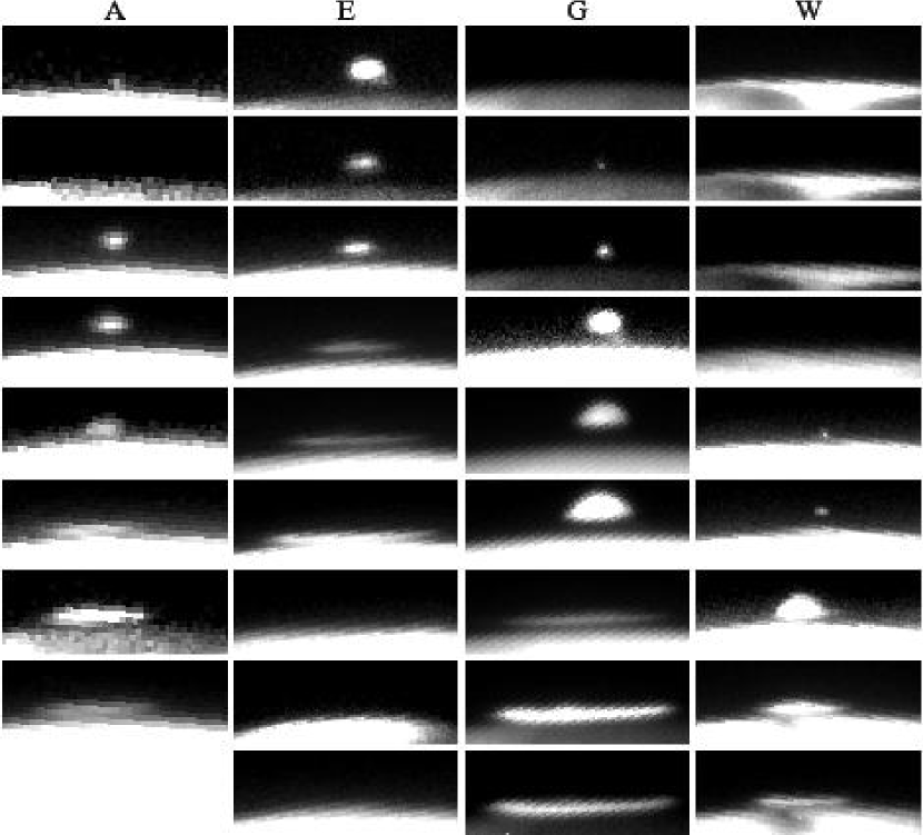
Figure 1: HST images plumes from the A, E, G, and W impacts, respectively, seen on Jupiter’s limb. The plumes continued to slide after they had fully collapsed. Note emission from the hot ejection tube in the first E and fourth G images.

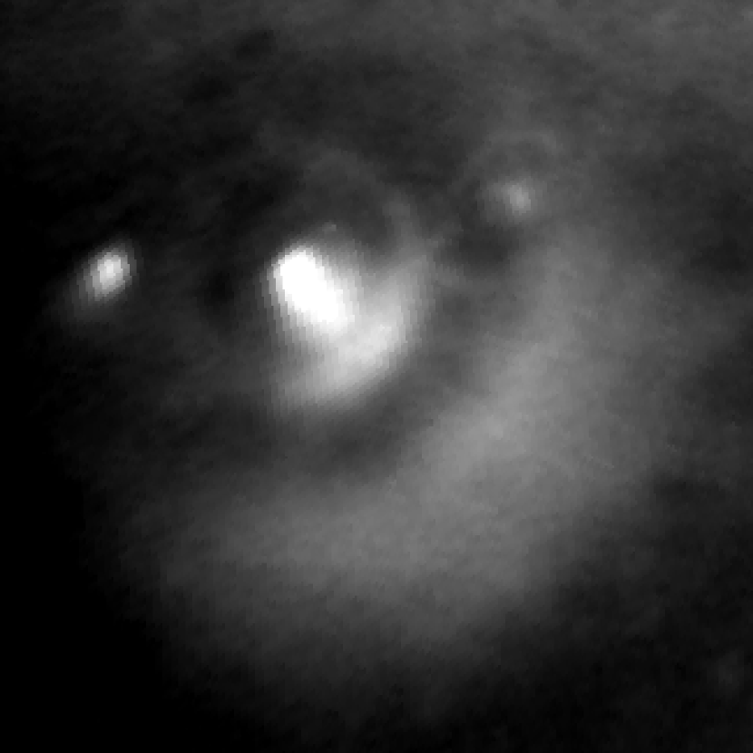
Figure 2: The G impact site, orthographic projection. Debris is bright in this 889 nm methane band HST image. The impact site is at the center of the complete ring, which is a propagating wave. It is located just inside the northwest portion of the streak region. The inner edge of the crescent slid less near the axis of symmetry than away from it, whereas the outer edge slid more near the axis. The tiny D impact streak is on the left.

Plume flight is a phase in its own right. The Hubble Space Telescope observed four plumes (impacts A, E, G, and W, HAM95). Jessup et al. (2000) calculated maximum altitudes of 2,300–3,100 km for material visible in these plumes. This region is so rarefied that hydrodynamics have minimal effect in the 20 minutes or so of flight, and ballistics dominate (ZM95). Initially, a plume is so hot it emits in the visible: the Galileo Photopolarimeter Radiometer and Ultraviolet Spectrometer both measured emission at 8,000 K (Carlson et al., 1997). This emission caused the “second precursors” in the observed lightcurves (Boslough et al., 1995). However, adiabatic expansion quickly cools the ejected gas to a few K, and the lightcurves are again quiet. Shoemaker et al. (1995) suggest a maximum flight time of only 10 minutes, but the observations show otherwise. The Sandia group ran their entry-response model through the plume phase, but stopped short of presenting the atmospheric re-entry boundary conditions or detailed impact images, as we do here. However, their code is capable of modeling the hydrodynamics relevant in the early part of this phase, which we cannot.

The present work, Pankine & Ingersoll (1999), and ZM95 all simplify the physics to ballistics at this stage. ZM95 justifies this simplification analytically. Intuitively, the pressures in the early stages of expansion into a vacuum are much larger than any others that will be encountered. The initial accelerations will dominate subsequent ones except those that act over long periods of time. After the initial expansion, the only consistent force is gravity, as pressure drops with volume and volume increases as the cube of time (faster, in the first seconds when hydrodynamics are relevant). The purposes of the three models diverge at this point. ZM95’s Monte-Carlo ballistic model is a vertical 2D sheet, and was used to study lightcurves and chemistry. Pankine & Ingersoll (1999) constrain plume sizes by parametric simulation of sliding under Coriolis influence. We calculate the boundary conditions for the atmospheric response. The present work, Pankine & Ingersoll (1999), the Sandia group, and the SPH group all calculate synthetic impact-site views.

In the landing response phase, falling plume material compressed itself and the ionosphere and upper stratosphere until they radiated, causing the entirely forseeable and quite unpredicted “main event” in the lightcurves (Zahnle, 1996). Shocks travelled up through the infalling plume material and down into the atmosphere. The infalling material deposited its vertical momentum, but continued its horizontal motion for many minutes, sliding on the atmosphere (HAM95, Jessup et al., 2000). At wavelengths near 0.9 mm, a brief “flare” appeared and vanished 1000 seconds after impact (Schleicher et al., 1994; Fitzsimmons et al., 1996; Ortiz et al., 1997), coincident with spectral observations of hot CO (Meadows & Crisp, 1995). In some lightcurves the flare briefly outshone the main event. The lightcurves then fell nearly as quickly as they rose, but not completely back to their initial level. They oscillated or “bounced” several times with a 10-minute period (Nicholson et al., 1995), then decayed for tens of minutes, depending on the wavelength observed. At 1.25 and 2 hours after impact, McGregor et al. (1996) observed a ring with radii of 14,000 and 18,000 km, respectively, giving a mean expansion rate of nearly 1.5 km/s in this time period. We call this feature “McGregor’s Ring.”

Eventually, material velocities fell below the sound and then the wind speeds. An unknown process generated a dark material that remained high in the atmosphere in the shape of a large crescent. This debris pattern’s outer edge is $\sim$13,000 km from the largest impact sites. Its inner edge is located at $\sim$6,000 km. The symmetry axis that splits the crescent and contains the impact site is rotated 14°-21° from the surface track of the incoming fragment. Pankine & Ingersoll (1999) and Jessup et al. (2000) model this as a Coriolis effect during plume flight and sliding. The material is bright in methane bands (HAM95), indicating a depth of just a few mbar (Molina et al., 1997). There is more material near the impact site itself, and (Walterscheid et al., 2000) claim the entry response rings are also made visible by this material. The largest impacts have rays pointing 1000–2000 km downrange from the impact site. These may be due to Rayleigh-Taylor instabilities in the earliest (pre-ballistic) plumes (HAM95). The debris crescent’s composition is uncertain (West et al., 1995) and it is still referred to by workers in the field as “the brown gunk.”

In the dissipation phase, material spreads with the winds, covering all longitudes in a few weeks and the southern mid-latitudes over several years, eventually fading from view (Banfield et al., 1996; Simon & Beebe, 1996).

HAM95 observed the plume material sliding on the atmosphere (see Fig. 1), an interpretation corroborated by the crescent locations. The G impact plume rose to $\sim$3,100 km (Jessup et al., 2000), but the outer crescent edge for that impact is $\sim$13,000 km from the impact site, more than twice as far as a ballistic object can fly under gravity, given this maximum height and assuming no bias in speed with ejection direction.

3 Ballistic Model

Ours is a Monte-Carlo ballistic model with parameterized sliding after reentry. At present we ignore Coriolis effects, planetary curvature, hydrodynamics, and thermodynamics. The model runs in two modes, called “fly” and “land”. Fly mode calculates the plume mass density at specific post-impact times in the volume of space above the impact site, creating views of the plumes in flight. Land mode calculates the plume re-entry mass, energy, and vertical momentum fluxes as a function of time and position on the surface. This mode both creates synthetic views of the final impact site and initializes our atmospheric response model (see Paper II).

We divide a plume into discrete, independent mass elements whose behavior is the same in both modes. Each element gets a random speed and direction. The model calculates the flight path and the time and location at which the element returns to its initial level. Upon landing, the element deposits its vertical momentum and slides horizontally until it stops, where it deposits its mass and energy. Both modes place a virtual grid of bins in the area of interest, and increment the appropriate bin when an element arrives. When the model has run the specified number of elements, it scales the bin values by volume and particle mass. In both modes one may choose either a rectangular or a spherical/polar grid, and may choose the minimum, maximum, and bin interval values independently on each axis. The impact site is the origin. In fly mode, the grid has three spatial dimensions, is evaluated at specific post-impact times, and accumulates only mass. In land mode, the grid is on the surface and thus has two dimensions spatially plus one temporally. It accumulates mass, energy, and vertical momentum.

The velocity distribution separates into independent direction and speed components. The ejection directions are uniformly distributed over the solid angle within a specified angle of the ejection channel axis. Figure 3 shows a cutaway view of this cone-like geometry.

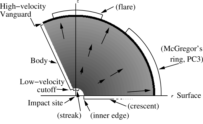
Figure 3: Plume cutaway diagram. All mass is instantaneously ejected up into a cone from the impact site, which is located at its (downward-pointing) apex. Vectors in the plume body indicate initial velocities. This side view shows a plume’s principal parts, the surface effects to which they give rise, and (schematically) the mass-velocity distribution. The instantaneous ejection implies that each plume element “sees” all other elements moving away with velocities proportional to their distances. There is thus no friction.

Figure 4: Top: Cumulative velocity distribution of ZM95, as modified for our model. Bottom: Differential velocity distribution used in the present model, with outer mass shell (derived in text). Cumulative and differential mass are in the same arbitrary units, which scale with $k$.

The model has two different MVDs. The first is the uniform distribution between two cutoff velocities. The second is an analytical model for the distribution that fits the numerical experiments of ZM95 very well (see their Fig. 3 and our Fig. 4). We chose the ZM95 distribution because it is the only one published in a form that is conducive to further modelling; most others only published synthetic images of specific energy or temperature and none published plots of mass vs. velocity. The ZM95 distribution also closely follows theoretical distributions for hypervelocity impact ejecta (ZM95 reviews theory and its applicability to this problem). Further, ZM95 developed the analytical approximation to their numerical distribution themselves, making clear their interpretation of their own numerical data:

$$M(>v)=\left\{\begin{array}[]{r@{\quad:\quad}l}kv^{-\alpha}&v\leq v_{\mbox{\scriptsize max}}\\ 0&v>v_{\mbox{\scriptsize max}}\end{array}\right.,$$ (1)

where $M(>v)$ is the mass moving at speeds greater than $v$, $k$ is a constant (see below), $v_{\mbox{\scriptsize max}}$ is the cutoff velocity seen in Fig. 4, and $\alpha$ is a constant between 1 and 2, constrained to that range by conservation considerations. The data in ZM95’s Fig. 3 give $\alpha=1.55$. This model approaches infinite mass at low velocity, but the energy is finite.

Cumulative distributions can make it difficult to visualize how the mass is distributed: just how much more mass exists between 1 and 2 km/s than between 9 and 10 km/s? A differential distribution would be more helpful, and is necessary for modeling. Taking the derivative piecewise yields:

$$\frac{{\mathrm{d}}m}{{\mathrm{d}}v}=\left\{\begin{array}[]{r@{\quad:\quad}l}k\alpha v^{-\alpha-1}&v<v_{\mbox{\scriptsize max}}\\ 0&v>v_{\mbox{\scriptsize max}}\end{array}\right..$$ (2)

There is no leading minus sign because the sense of accumulation was $M(>v)$ rather than $M(<v)$ before taking the derivative, which changes the sign of the right side of Eq. 2. One discovers something peculiar about this distribution. If $M(>v)=0$ at speeds faster than $v_{\mbox{\scriptsize max}}$, how can it discontinuously be positive at $v<v_{\mbox{\scriptsize max}}$? The discontinuity in Eq. 1 yields a delta function in the derivative of size $M(>v_{\mbox{\scriptsize max}})$, which at first appears unphysical. One might be tempted to dispose of such a mathematical quirk, but ZM95’s Fig. 3 comes from the final data of a numerical SL9 impact model. It is not the result of computational peculiarities of that model and it is in line with a well-established theory. Their plotted line does not cut off abruptly, but rather drops off with a very steep slope ($\alpha\approx 6$), which still yields a spike in the derivative that integrates to $M(>v_{\mbox{\scriptsize max}})$. The spike appears as a dense outer shell of gas in Fig. 4 of Ahrens et al. (1994a), which shows the effect to be greater for larger fragments. We hypothesize that this shell is the remnant of the shock wave and compressed upper atmosphere that preceeded the main body of the plume into space. We call this spike of mass the plume “vanguard,” since it is the first plume material to reach any given point and since its effect upon landing is similar to that of its namesake.

As we discuss below, the vanguard contains 22% of the mass and 45% of the energy in the model plumes whose final appearance best matches the HST data. We find below that it explains McGregor’s ring, a finding confirmed more rigorously in Paper II. That paper further finds that it produces the “third precursor” (PC3) and flare features of the lightcurves (Fitzsimmons et al., 1996). McGregor’s ring and the flare are absent in runs without a vanguard. We also note that the vanguard is similar to the single mass shell found by Pankine & Ingersoll (1999) to match their data well. Finally, we point out that a density enhancement is often seen immediately behind shocks (e.g., see the shock tube test of Paper II) and would therefore not be a surprising feature of the initial plume expansion.

To create post-impact views with a debris crescent (see below), we also introduce a minimum velocity ($v_{\mbox{\scriptsize min}}$), which may be zero for the flat distribution but must be positive for the power-law distribution. One physical justification for a minimum velocity cutoff is the “pinching off” at the 1-bar level suggested by Boslough et al. (1995) to explain why the plumes all rose to the same height. Another, suggested by Zahnle et al. (1995), is that carbonaceous grains, which may be the brown gunk, can be formed by material impacting faster than 4.5 km/s. This cutoff does not introduce any further complications into the differential distribution used in the model. We call the final distribution “cumulative power law with cutoff”, or CPC:

$$\begin{array}[]{lr}\lx@intercol\@ADDCLASS{ltx_eqn_lefteqn}$\displaystyle\frac{{\mathrm{d}}m}{{\mathrm{d}}v}=$\mbox{}\hfil\lx@intercol&\\[8.61108pt] \left\{\begin{array}[]{r@{\;:\;}l}k(\alpha v^{-\alpha-1}+v_{\mbox{\scriptsize max}}^{-\alpha}\delta(v-v_{\mbox{\scriptsize max}}))&v_{\mbox{\scriptsize min}}\leq v\leq v_{\mbox{\scriptsize max}}\\ 0&\mbox{otherwise.}\end{array}\right.\end{array}$$ (3)

To assign each particle a velocity, we first calculate $m_{\mbox{\scriptsize van}}/m_{\mbox{\scriptsize plume}}$, where $m_{\mbox{\scriptsize van}}=M(>v_{\mbox{\scriptsize max}})$ and $m_{\mbox{\scriptsize plume}}=M(>v_{\mbox{\scriptsize min}})$, and assign $v_{\mbox{\scriptsize max}}$ to that fraction of the particles. For the remaining particles, we integrate Eq. 3 from $v_{\mbox{\scriptsize min}}$ to $v^{\prime}$ and divide by the total mass to give an expression for $M(<v^{\prime})$ with our particular $v_{\mbox{\scriptsize min}}$, and solve for $v^{\prime}$. This gives the velocity probability distribution in terms of a uniformly distributed random variable, $r$, whose range is 0–1:

$$v(r)=\left(v_{\mbox{\scriptsize min}}^{-\alpha}-r(v_{\mbox{\scriptsize min}}^{-\alpha}-v_{\mbox{\scriptsize max}}^{-\alpha})\right)^{-\frac{1}{\alpha}}$$ (4)

A random number generator provides uniformly-distributed numbers, which we scale to the range 0–1.

We randomly assign a particle’s azimuth and deflection ($\theta$) around an initially vertical axis, then convert to rectangular coordinates and rotate the direction vector to the axis inclination and azimuth specified for the plume. The distribution of azimuth at a given axis deflection is inherently uniform in polar coordinates, so we simply rescale the random numbers to the range 0–$2\pi$. The histogram of $\theta$ is proportional to the circumference of circles of constant $\theta$, and we follow a similar procedure to the derivation of Eq. 4 to create an appropriate function of $r$ and the opening angle $\theta^{\prime}$:

$$\theta(r)=\cos^{-1}\left[1-r(1-\cos\theta^{\prime})\right].$$ (5)

The constant $k$ embodies the bulk impact physics other than the MVD and geometry. This number characterizes the density of the plume and the amount of entrained Jovian air. It scales with the impactor mass ($m_{i}$), velocity ($v_{i}$), and the fraction of impactor kinetic energy going into the plume ($\eta$). Following ZM95 but including the mass in the vanguard, we set the total available energy equal to that in the plume:

$$\frac{\eta m_{i}v_{i}^{2}}{2}=\int_{v_{\mbox{\scriptsize min}}}^{v_{\mbox{\scriptsize max}}}\frac{{\mathrm{d}}m}{{\mathrm{d}}v}\frac{v^{2}}{2}{\mathrm{d}}v.$$ (6)

Substituting $\frac{{\mathrm{d}}m}{{\mathrm{d}}v}$ from Eq. 3 and solving for $k$ gives:

$$k=\frac{\eta m_{i}v_{i}^{2}(2-\alpha)}{2v_{\mbox{\scriptsize max}}^{2-\alpha}-\alpha v_{\mbox{\scriptsize min}}^{2-\alpha}}.$$ (7)

For comparison to ZM95, the cumulative mass with $v_{\mbox{\scriptsize min}}$=0 is

$$M(>v)=\frac{2-\alpha}{2}\eta m_{i}\left(\frac{v_{i}}{v_{\mbox{\scriptsize max}}}\right)^{2}\left(\frac{v_{\mbox{\scriptsize max}}}{v}\right)^{\alpha},$$ (8)

and $m_{\mbox{\scriptsize van}}$ is just this with $v=v_{\mbox{\scriptsize max}}$. This differs from ZM95’s equation 9 only in the replacement of $\alpha$ with 2 in the first denominator. The expression for vanguard energy $e_{\mbox{\scriptsize van}}$ under the $v_{\mbox{\scriptsize min}}$=0 assumption is

$$e_{\mbox{\scriptsize van}}=\frac{\eta m_{i}v_{i}^{2}}{2}\left(1-\frac{\alpha}{2}\right).$$ (9)

Only $v_{i}$ is observationally constrained, at about 60 km/s. The product $\eta m_{i}$ is not directly constrained by this model, nor do any results presented in this paper depend on it. ZM95 state that their impact models are consistent with values in the range $0.3\leq\eta\leq 0.45$, but in their discussion they allow values as low as 0.01. Bezard et al. (1997) estimate $\eta>0.2$ for the L impact. We use $\eta$=0.3. The mass $m_{i}$ is one of the holy grails of SL9 post-impact work (Carlson et al., 1997). Our nominal value is 1.4$\times$1014 g, which is justified in Paper II based on lightcurve intensity levels and ZM95’s $\eta$. Plume mass density and the plume re-entry fluxes of mass, energy, and momentum are all linearly proportional to $k$, which is in turn independent of $v$. We thus compute the entire model using counting bins that “catch” particles of unit mass, and multiply the bins by a scale factor that includes $k$ at the end of the computation. This allows flexibility in choosing the value of $\eta m_{i}$, as the entire grid can again be multiplied by a scale factor until models based on it produce synthetic observables most in line with observations. This can be done without rerunning the model.

For consistency with ZM95, we evaluate $k$ under the assumption of an MVD running from 0 to $v_{\mbox{\scriptsize max}}$. This only affects the total mass, which we take as unconstrained and will later fit. The relative size of the vanguard and the rest of the distribution remains the same.

Upon landing and in land mode only, the particles deposit their vertical momentum at the azimuth, radial distance ($r_{l}$), and time ($t_{l}$) of landing, and slide with initial horizontal velocity $v_{h}$ following one of three schemes: no sliding, constant time, and constant deceleration. The sliding schemes calculate the distance ($r_{s}$) and duration ($t_{s}$) of sliding, and deposit particle mass and kinetic energy at $r_{l}+r_{s}$, $t_{l}+t_{s}$, and the landing azimuth. We carry the energy along because we expect most of it to convert to heat, which slides with the particle.

In the “no sliding” scheme, all quantities are deposited at the landing location and time. “Constant-time” sliding was inspired by conference discussions reporting that sliding occurred for about $t_{s}$=20 minutes after impact, based on a quick look at the HST data. Particles travel $r_{s}=t_{s}v_{h}$. With constant deceleration $f$, $r_{s}=v_{h}^{2}/2f$ and $t_{s}=v_{h}/f$.

4 Model Runs and Discussion

The previous section makes it apparent that the model has a large number of adjustable parameters. However, direct observations constrain many of their values and the input velocity distribution (based on prior models) constrains several others. Most of the remainder have identifiable, independent effects on the debris pattern views, and this independence reduces the volume of reasonable phase space dramatically.

Table 2: Model Parameters

Description	Symbol	Value	Units	Constraint
gravity	$g$	23.25	m/s2	orbits, day length, latitude
impactor velocity	$v_{i}$	60	km/s	Chodas & Yeomans (1996)
impactor mass	$m_{i}$	1.4$\times$1014	g	paper II
plume energy fraction	$\eta$	0.3		ZM95
opening angle	$\theta$	75	°	fit
axis azimuth (N $\rightarrow$ E)		145	°	HAM95
axis tilt from normal		30	°	fit
mass-velocity distribution	CPC, flat			fit, ZM95
mass-velocity power law	$\alpha$	1.55		fit, ZM95
low velocity cutoff	$v_{\mbox{\scriptsize min}}$	4.5	km/s	fit, Carlson et al. (1995)
max particle velocity	$v_{\mbox{\scriptsize max}}$	11.81	km/s	HAM95
sliding scheme	const. deceleration			fit
sliding time constant		0	s	fit
deceleration		1.74	m/s2	fit
observed first re-entry time	$t_{min}$	350	s	Carlson et al. (1995)
observed max plume altitude	$z_{max}$	3,000	km	HAM95

2

Table 2 summarizes the variable parameters and sources of observational constraint and presents the values in our nominal plume. The values of $m_{i}$ and $\eta$ are very uncertain but do not affect the appearance of the debris-field views in this model. In practice, the final step of the model divides all particle counting bin values by the total number of particles and multiplies by $\eta m_{i}$. However, in Paper II we discuss lightcurves, where the total mass matters quite a bit. Pankine & Ingersoll (1999) constrain plume masses directly with their model of Coriolis-modified sliding (but see below). A direct estimate of plume mass from the HST debris images might be possible, but only after the determination of the composition, optical properties, and means of forming the brown gunk that makes the debris field visible. This is one of the principal unsolved puzzles of the SL9 impacts (West et al., 1995).

The ejection altitude is the level at which ballistics dominates hydrodynamics in the emerging plume. To well within the 800-km range in the four measured plume heights (Jessup et al., 2000), this is about the level at which re-entering material will start to re-encounter significant hydrodynamic forces. Estimates of the terminal depth of the incoming fragment vary over 200–300 km (Borovička & Spurný, 1996; Crawford, 1996; Mac Low, 1996). Since the plume travels up the path of the incoming fragment, the early development of the entry channel and details of fragment breakup will affect the ejection altitude. However, these effects are small compared to the range in plume heights.

The rest of this section presents the relationship between parameters and observations, showing what happens to the debris-pattern views when we change parameter values. Each of the synthetic view panels in the figures presents 100 million Monte-Carlo particles cast onto a polar computational grid. Each grid had 100 radial bins between the impact site and the location of the most-distant debris (after sliding), 36 azimuthal bins, and a single time bin. Except as noted, the views here show the surface mass density as a linearly varying grayscale. Because different model parameters yield vastly differing peak densities and pattern sizes, we have scaled the intensities in each view separately. The total mass in any view varies only because of changes in the minimum velocity (except when we vary the velocity distribution), and that effect can be estimated by looking at Fig. 4.

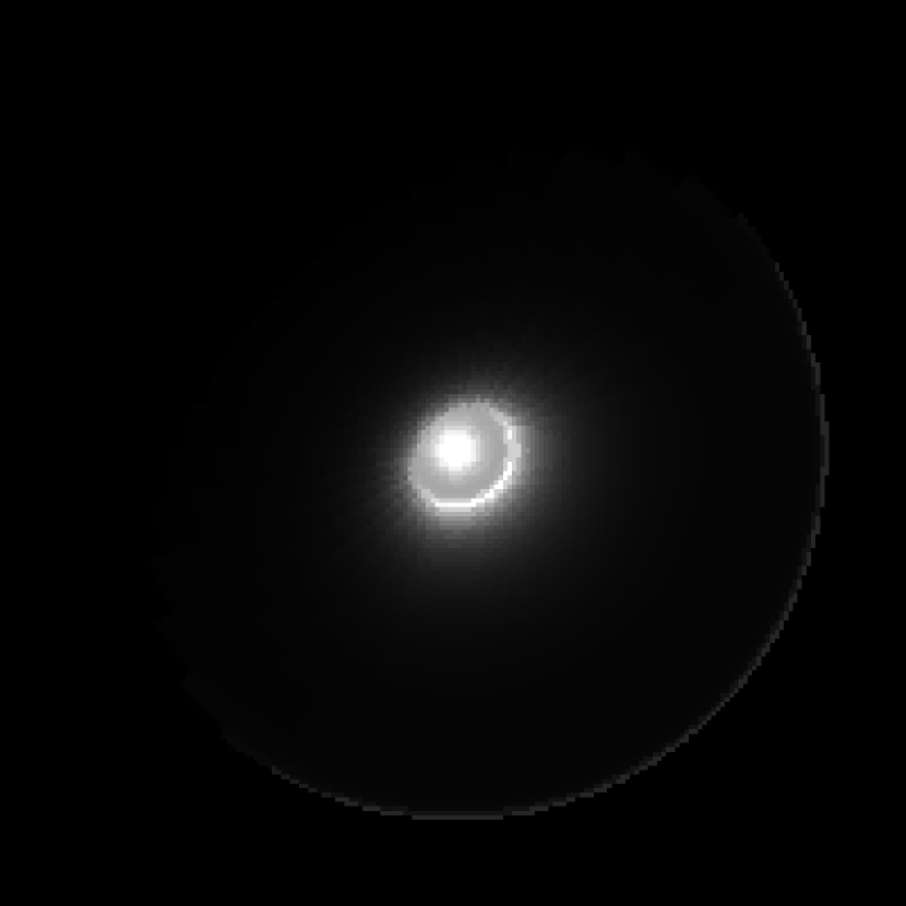
Figure 5: Best overhead view of the impact site after all material has come to rest. Intensity is proportional to mass deposited. Note that observed impact sites show dark grains, not the plume gas. The formation and redistribution of grains is still not well understood, so in these images the locations of particular features is more important than relative intensities. Table 2 gives model parameters, which were adjusted to match the appearance of Fig. 2. The inside of the debris crescent has slid 6,000 km from the impact site. The thin exterior ring has a very large radius (46,000 km) with our nominal sliding parameters. We identify the ring in our model with one observed to be expanding at nearly 1.5 km/sec 2 hours after impact by McGregor et al. (1996). The figure width is 100,000 km.

Figure 5 shows the scene from above when all material has come to rest, using the parameters in Table 2. The low-velocity cutoff produces a sharp inner crescent edge at 6,000 km. Vertically-ejected material landed near the impact site and stayed near it. This streak contains more mass than the remainder of the debris combined, which is consistent with the data in Fig. 2. The crescent is narrower than in the observations, which is likely due to the simplistic sliding applied here. McGregor’s ring has stopped 46,000 km from the impact site. We now adjust parameters away from this ideal to show why these are the best values.

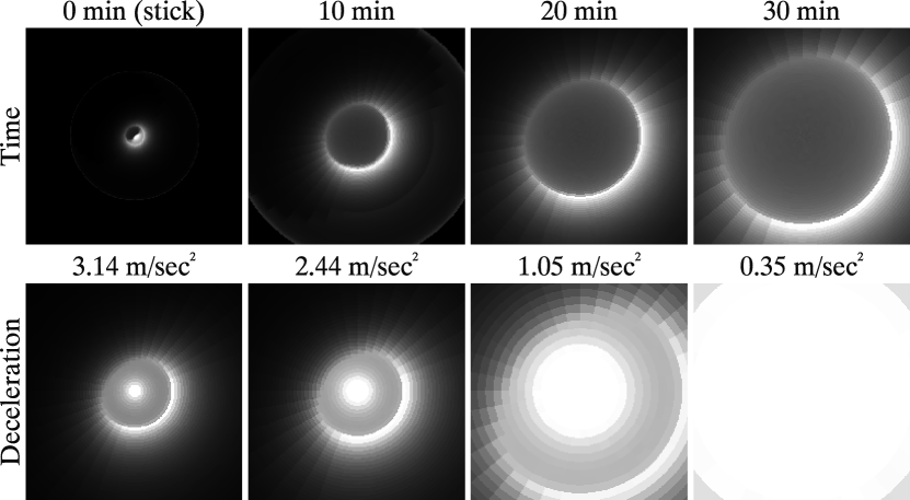
Figure 6: Effects of different types of horizontal sliding. Plot parameters are the same as in Fig. 5. The top-left frame has no sliding and demonstrates the requirement for sliding of some type, as purely ballistic motion does not deliver material nearly far enough from the impact site. In the remaining frames of the top row, each particle slid at its horizontal velocity for the indicated period of time. This is also not realistic because it does not form a central streak of material near the impact site. Material that flew vertically and thus had a very small horizontal velocity component slides for the same time as material ejected on horizontal trajectories, clearing the middle. The bottom row shows sliding with a constant deceleration that mimics work agains a constant pressure or sliding up a hill. This most closely matches the impact images. The parameters shown bracket the ideal parameter of Fig. 5. The panel width is 20,000 km. Vanguard material may be outside of a given frame, but we did not use its location as a criterion for estimating optimal parameters.

If we turn off sliding entirely, the top-left panel of Fig. 6 shows that the material does not spread far enough. The remaining figures in that row have constant-time sliding that fails to produce a streak region at all. Material ejected nearly vertically slides for too long and leaves the central region. Only the bottom row’s sliding with a constant deceleration does a reasonable job, making a dense streak and a well-defined crescent. The deceleration parameter determines where the crescent stops sliding, and the value 1.74 m/sec2 puts the inner edge at the observed 6,000 km. It is coincidental that the 20-minute sliding estimate happens also to put the inner edge near this location.

There are at least two relevant physical interpretations of constant deceleration: work against a constant pressure and sliding up a hill. In the hill analogy, the mass and momentum of the falling plume material compresses the atmosphere where it lands, but closer to the impact site there is much more material than further away. This creates a slope. Debris slides in the direction away from the impact site, trading kinetic energy for potential as it climbs the “hill”. Our 1.74 m/s2 deceleration corresponds to a hill pitch of 4.3°. In reality, the slope would vary with the amount of material that had already fallen at a given time and how it had moved, while our hill has a constant slope. In the pressure analogy, the expanding material must push against the surrounding atmosphere to expand. It encounters new, stationary material that it must accelerate throughout its expansion. In reality, the deceleration pressure depends on the instantaneous expansion velocity, radius, and the depth to which the plume has compressed the atmosphere, which varies with azimuth and distance from the impact site. Both hill and pressure effects may play a role in stopping the debris.

In contrast to our constant deceleration, Pankine & Ingersoll (1999) use a per-particle force proportional to $v^{2}$ that would be appropriate for viscous drag. Monte-Carlo particle models such as ours and theirs ignore the fact that only a small amount of material is involved in the turbulent boundary layer between the sliding plume and the stationary atmosphere, and material above this interface would continue sliding unabated until the turbulent mixing length scale was as large as the depth of the fallen plume material, which is deep (Paper II). A better tool for studying horizontal expansion is a fluid model, and we take up the question more realistically in Paper II, initializing with unslid plumes. Both our scheme and that of Pankine & Ingersoll (1999) work as simple ways to simulate the appearance of the data and to explore plume parameters, but one must be cautious if using either model beyond that point.

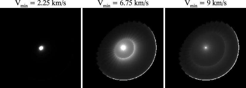
Figure 7: Effect of varying the minimum plume velocity. Plot parameters are the same as in Fig. 5. The parameters shown bracket the ideal parameter of Fig. 5. Changing this parameter changes the location of the inner crescent edge and the fraction of material near the impact site. The panel width is 100,000 km.

Changes in $v_{\mbox{\scriptsize min}}$ do three things: first, they alter the relative fraction of material in the streak, with lower $v_{\mbox{\scriptsize min}}$ increasing the mass in the center; second, they change the location of the inner crescent edge; and third, they change the landing time of plume body material ejected on vertical paths. One can adjust $v_{\mbox{\scriptsize min}}$ and the sliding deceleration to keep the inner crescent edge in the same location but change the relative streak and crescent distributions. However, doing so also changes the start time of the lightcurve main event.

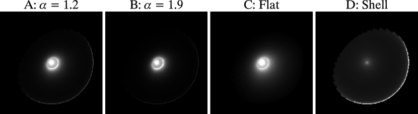
Figure 8: Different velocity distributions. Plot parameters are the same as in Fig. 5. A & B: ZM95 power-law with parameter $\alpha$ that brackets the ideal parameter of Fig. 5. C: Flat distribution between ideal cutoff velocities. Its morphology is similar to that of panels A and B, but with a sparser central region and no exterior ring. D: Shell distribution, essentially a delta function with velocity $v_{\mbox{\scriptsize max}}$. It does not resemble the data. The panel width is 20,000 km.

As Fig. 8 shows, changing the power law parameter $\alpha$ does not have a dramatic effect, but it does alter the width of the crescent and the relative amounts of material in the crescent and streak. Using a flat distribution eliminates the exterior ring feature, and would eliminate our ability to match observations of PC3 and the flare with synthetic lightcurves in the next impact phase and would leave McGregor’s ring unexplained. A shell distribution (a flat distribution with $v_{\mbox{\scriptsize min}}$ close to $v_{\mbox{\scriptsize max}}$) eliminates the crescent. There is a streak because vertically-ejected material still does not slide, but it is very small. CPC is the only distribution that puts material in all three places where it is observed: a central condensation, a crescent, and McGregor’s ring. It also produces realistic lightcurves (Paper II). Pankine & Ingersoll (1999) conclude that a shell distribution is more realistic than their roughly-Gaussian distribution. Note that our respective crescents are produced by different phenomena: theirs is from the shell and is spread out radially by $v^{2}$ drag, ours is from CPC’s low-velocity cutoff. Our shell produces McGregor’s ring, and our constant-force sliding does not spread it very much.

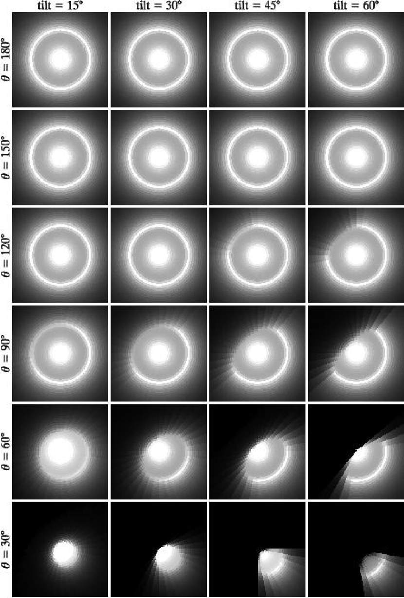
Figure 9: Geometry changes. Plot parameters are the same as in Fig. 5. Ejection axis angle from the vertical varies across the rows as indicated, and opening angle (axis to cone side) varies down the columns. A 180° opening angle is a spherical distribution. The panel width is 20,000 km, which puts vanguard material outside the frame. In all cases, it is thin, circular, and has an azimuthal mass distribution roughly in proportion to the mass interior to it, though it tends to cover more azimuth than the interior material.

Changing the cone geometry, as shown in Fig. 9, has dramatic effects. The decidedly non-circular site appearance (see Fig. 2) requires a tilted axis, but the 45° tilt of the impactor’s entry path (tilt = 45° column of Fig. 9) is too much. Our best axis is 30° from normal, exactly halfway between Crawford’s (1996) 20° and Takata & Ahrens’s (1997) 40° values. Pankine & Ingersoll (1999) use the entry path as the ejection axis. The opening angle is similarly important. A small opening angle is like a constrained jet, whereas a large one makes the debris pattern too circular. We find 75° from axis to cone edge best reproduces the data, in good agreement with Pankine & Ingersoll’s (1999) 70°. We do not understand how Takata & Ahrens’s (1997) ejecta pattern, which spans well over 120° in their Fig. 7, could have been generated from non-interacting ballistic particles ejected $\pm$30° from the bolide entry path and rotating only the stated 15° due to Coriolis effects.

5 Nominal Plume Characteristics and Atmospheric Modeling Considerations

The distribution of mass, kinetic energy, and momentum flux in the nominal plume infall is sharply time-dependent. Fig. 10 shows the three quantities as well as a 3-dimensional view as a function of time. The main event, which peaks at 600 sec (Nicholson et al., 1995), is radiation due to the arrival of kinetic energy. The lightcurves’ PC3 corresponds to the early, nearly-horizontal expansion of the vanguard through the atmosphere. The final collapse of the vanguard around 1000 sec causes the transient flare in the $\sim$0.9mm lightcurves. Paper II covers both topics in more detail. Figure 11 shows the azimuthally-integrated mass distribution after all material has stopped. Figure 12 gives the mass and kinetic energy fallen as a function of time.

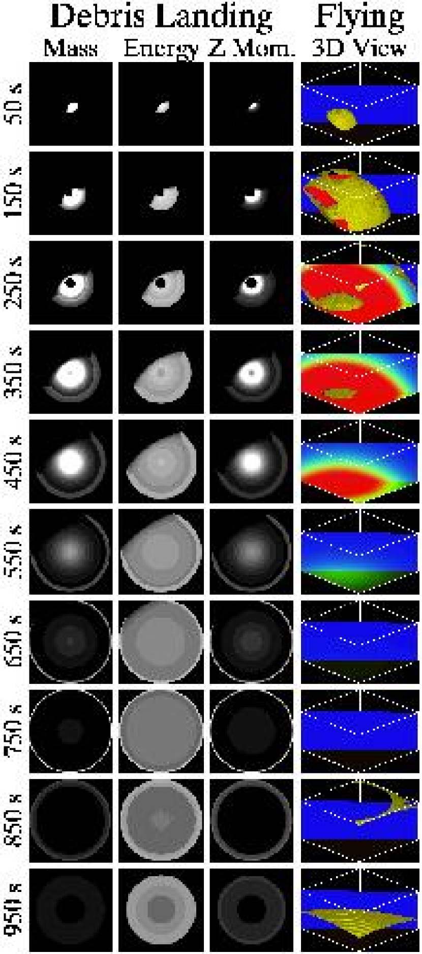
Figure 10: Left columns: Overhead views of mass, energy, and vertical momentum deposited in Jupiter’s atmosphere by an SL9 impact plume, over time. This model run has no sliding. Each landing quantity has the same log-scaled grayscale throughout its column. Early landing views are saturated so that later views can be seen at all. The patterns and deposition peaks differ. Mass peaks early, energy is strong throughout, and momentum peaks in mid-plume. The panel width is 12,000 km. Right column: 3D rendering of a plume in flight, viewed from above the southwest. The rendering shows a yellow isosurface of mass density (in this case nearly a material surface) and two planes showing mass density. These planes are the $z$=0 level and the vertical plane containing the plume axis. The latter has been colored blue at zero density as an aid to viewing. Rendering only inside the indicated box makes the interior density gradient visible.

According to Eq. 8, a plume entrains 10–100 impactor masses of Jovian air. The uncertainty comes from the unknown $\eta$ and the question of what low-end velocity to choose as the cutoff value for the plume (without which it contains infinite mass). With ZM95’s arbitrary $\eta$ = 0.3 and vmin = 1 km/s, a plume entrains 80 impactor masses of air. The amount of entrainment scales linearly with $\eta$. For vmin = 2 km/s, the entrainment is 27 $m_{i}$ and for vmin = 4.5 km/s it is 7.8 $m_{i}$. Ahrens et al. (1994a) and Takata et al. (1994) calculate values of 20 and 40 $m_{i}$ for their 2-km fragment. Even with the extremes of temperature and pressure experienced by plume gas, molecular hydrogen is so dominant that values for the molecular weight of infallen plume material should be close to that of Jovian air.

Figure 11: Mass as a function of radius, integrated over azimuth, after sliding has stopped. Definite integrals of this function give the mass in each part of the debris field.

Figure 12: Rate of total mass and energy impacting the atmosphere (no sliding) as a function of time. Compare to the lightcurve shown in Fig. 8 of Paper II. The spike at 740 sec corresponds to the onset of CO emission observed by Meadows & Crisp (1995).

Crawford (1996) present evidence in their Fig. 9 that the visible portion of the plumes are due to a lofted cloud deck, and that there may be invisible portions that went many times higher. We set $v_{\mbox{\scriptsize max}}$ based on the observed $\sim$3,000 km maximum altitudes (Jessup et al., 2000), but could set it arbitrarily and adjust sliding parameters accordingly. However, in Paper II we present a lightcurve match based on our nominal parameters.

6 Conclusions

We initialize a plume model with the final conditions of an entry-response model, preserving the physical state as much as possible as we transition from one set of dominant physics to the next. In so doing, we have discovered physical explanations for a number of disparate, previously-unexplained phenomena, including McGregor’s ring, PC3, and the flare. All of these phenomena depend on the details of the geometry and the initial conditions: reduced-dimension models and most “reasonable” assumed initial conditions will not reproduce them.

The parameter phase space for SL9 impact plumes is large. However, by using the ballistic approximation, we can determine reasonable values for the geometry and the velocity distribution. Comparison of our best debris-field view to the actual data still leaves us short of perfection. The differences are likely due to non-ballistic effects in the very young plume, the details of grain formation, and the hydrodynamic details of post-reentry silding. Models that can calculate these effects are much more complicated than this one, and exploring phase space with such a model is computationally prohibitive. However, those with such models may safely restrict their investigations to geometry, velocity distribution, and sliding that is consistent with the nominal parameters given in Table 2. We encourage workers who wish to use the quantities presented here to contact us for numerical versions.

We leave a number of questions for future work. Modifications to take into account the planet’s roundness and rotation would delay infall of material away from the impact site. Coriolis effects in flight and in sliding would rotate the patterns. Finally, there are likely still things to learn from direct analysis of the plumes in flight (see Fig. 1), especially when compared to models.

We postulate a particular velocity distribution to explain the features of the SL9 impact sites. Images of the sites are static (except for the waves), and possibly other distributions could produce the same or better pictures. However, we also have timing observations in the forms of both light curves and spectra, and we have not tuned any plume parameters to match them, except to set $v_{\mbox{\scriptsize min}}$ as suggested by Carlson et al. (1995). In Paper II we take up a thorough test of the plume presented here, dropping it onto a radiative-hydrodynamic atmosphere model that creates synthetic light curves. We compare those light curves to the observations, making this the first detailed model of plume collapse on an atmosphere that is constrained by observation of an actual collapsing plume.

Although SL9 was a once-in-a-lifetime event, lifetimes are short, and impacts are common and important in our solar system’s history. We view the SL9 impacts not as a one-time curiosity, but as a vital window on processes that shaped the Earth and planets. We are excited by the prospect of the next large plume event, and entertain the notion that it may be man-made.

References

- Ahrens et al. (1994a) Ahrens, T. J., Takata, T., O’Keefe, J. D., & Orton, G. S. 1994a, Geophys. Res. Lett., 21, 1087
- Ahrens et al. (1994b) —. 1994b, Geophys. Res. Lett., 21, 1551
- Banfield et al. (1996) Banfield, D., Gierasch, P. J., Squyres, S. W., Nicholson, P. D., Conrath, B. J., & Matthews, K. 1996, Icarus, 121, 389
- Bezard et al. (1997) Bezard, B., Griffith, C. A., Kelly, D. M., Lacy, J. H., Greathouse, T., & Orton, G. 1997, Icarus, 125, 94
- Borovička & Spurný (1996) Borovička, J. & Spurný, P. 1996, Icarus, 121, 484
- Boslough et al. (1995) Boslough, M. B., Crawford, D. A., Trucano, T. G., & Robinson, A. C. 1995, Geophys. Res. Lett., 22, 1821
- Carlson et al. (1997) Carlson, R. W., Drossart, P., Encrenaz, T., Weissman, P. R., Hui, J., & Segura, M. 1997, Icarus, 128, 251
- Carlson et al. (1995) Carlson, R. W., Weissman, P. R., Hui, J., Segura, M., Smythe, W. D., Baines, K. H., Johnson, T. V., Drossart, P., Encrenaz, T., Leader, F., & Mehlman, R. 1995, in ESO Conf. and Wrokshop Proc. 52, European SL-9/Jupiter Workshop, ed. R. West & H. Bönhardt (Garching bei München, Germany: European Southern Observatory), 69
- Chodas & Yeomans (1996) Chodas, P. W. & Yeomans, D. K. 1996, in IAU Colloq. 156, The Collision of Comet Shoemaker-Levy 9 and Jupiter, ed. K. S. Noll, H. A. Weaver, & P. D. Feldman (Cambridge, UK: Cambridge University Press), 1
- Crawford (1996) Crawford, D. A. 1996, in IAU Colloq. 156, The Collision of Comet Shoemaker-Levy 9 and Jupiter, ed. K. S. Noll, H. A. Weaver, & P. D. Feldman (Cambridge, UK: Cambridge University Press), 133
- Crawford et al. (1994) Crawford, D. A., Boslough, M. B., Trucano, T. G., & Robinson, A. C. 1994, Shock Waves, 4, 47
- Deming & Harrington (2001) Deming, D. & Harrington, J. 2001, ApJ, submitted
- Fitzsimmons et al. (1996) Fitzsimmons, A., Andrews, P. J., Catchpole, R., Little, J. E., Walton, N., & Williams, I. P. 1996, MNRAS, 278, 781
- Hammel et al. (1995) Hammel, H. B., Beebe, R. F., Ingersoll, A. P., Orton, G. S., Mills, J. R., Simon, A. A., Chodas, P., Clarke, J. T., de Jong, E., Dowling, T. E., Harrington, J., Huber, L. F., Karkoschka, E., Santori, C. M., Tiogo, A., Yeomans, D., & West, R. A. 1995, Science, 267, 1288
- Harrington et al. (1994) Harrington, J., Le Beau, R. P., Backes, K. A., & Dowling, T. E. 1994, Nature, 368, 525
- Ingersoll & Kanamori (1995) Ingersoll, A. P. & Kanamori, H. 1995, Nature, 374, 706
- Jessup et al. (2000) Jessup, K. L., Clarke, J. T., Ballester, G. E., & Hammel, H. B. 2000, Icarus, 146, 19
- Mac Low (1996) Mac Low, M.-M. 1996, in IAU Colloq. 156, The Collision of Comet Shoemaker-Levy 9 and Jupiter, ed. K. S. Noll, H. A. Weaver, & P. D. Feldman (Cambridge, UK: Cambridge University Press), 157
- McGregor et al. (1996) McGregor, P. J., Nicholson, P. D., & Allen, M. G. 1996, Icarus, 121, 361
- Meadows & Crisp (1995) Meadows, V. & Crisp, D. 1995, in ESO Conf. and Wrokshop Proc. 52, European SL-9/Jupiter Workshop, ed. R. West & H. Bönhardt (Garching bei München, Germany: European Southern Observatory), 239
- Molina et al. (1997) Molina, A., Moreno, F., & Munoz, O. 1997, Icarus, 127, 213
- Nicholson et al. (1995) Nicholson, P. D., Gierasch, P. J., Hayward, T. L., McGhee, C. A., Moersch, J. E., Squyres, S. W., van Cleve, J., Matthews, K., Neugebauer, G., Shupe, D., Weinberger, A., Miles, J. W., & Conrath, B. J. 1995, Geophys. Res. Lett., 22, 1613
- Ortiz et al. (1997) Ortiz, J. L., Orton, G., Moreno, F., Molina, A., Larson, S., & Yanamandra-Fisher, P. 1997, A&A, 324, 357
- Pankine & Ingersoll (1999) Pankine, A. A. & Ingersoll, A. P. 1999, Icarus, 138, 157
- Schleicher et al. (1994) Schleicher, H., Balthasar, H., Knolker, M., Schmidt, W., & Jockers, K. 1994, Earth Moon and Planets, 66, 13
- Shoemaker et al. (1995) Shoemaker, E. M., Hassig, P. J., & Roddy, D. J. 1995, Geophys. Res. Lett., 22, 1825
- Simon & Beebe (1996) Simon, A. A. & Beebe, R. F. 1996, Icarus, 121, 319
- Takata & Ahrens (1997) Takata, T. & Ahrens, T. J. 1997, Icarus, 125, 317
- Takata et al. (1994) Takata, T., O’Keefe, J. D., Ahrens, T. J., & Orton, G. S. 1994, Icarus, 109, 3
- Walterscheid et al. (2000) Walterscheid, R. L., Brinkman, D. G., & Schubert, G. 2000, Icarus, 145, 140
- West et al. (1995) West, R. A., Karkoschka, E., Friedson, A. J., Seymour, M., Baines, K. H., & Hammel, H. B. 1995, Science, 267, 1296
- Zahnle (1996) Zahnle, K. 1996, in IAU Colloq. 156, The Collision of Comet Shoemaker-Levy 9 and Jupiter, ed. K. S. Noll, H. A. Weaver, & P. D. Feldman (Cambridge, UK: Cambridge University Press), 183
- Zahnle & Mac Low (1994) Zahnle, K. & Mac Low, M.-M. 1994, Icarus, 108, 1
- Zahnle & Mac Low (1995) —. 1995, J. Geophys. Res., 100, 16885
- Zahnle et al. (1995) Zahnle, K., Mac Low, M.-M., Lodders, K., & Fegley, B. 1995, Geophys. Res. Lett., 22, 1593