Dwarf Elliptical Galaxies:
Structure, Star Formation, and Color-Magnitude Diagrams

Abstract

The aim of this paper is to cast light on the formation and evolution of elliptical galaxies by means of N-body/hydro-dynamical simulations that include star formation, feed-back and chemical evolution. Particular attention is paid to the case of dwarf spheroidals of the Local Group which, thanks to their proximity and modern ground-based and space instrumentation, can be resolved into single stars so that independent determinations of their age and star formation history can be derived. Indeed, the analysis of the color-magnitude diagram of their stellar content allows us to infer the past history of star formation and chemical enrichment thus setting important constraints on galactic models. Dwarf galaxies are known to exhibit complicated histories of star formation ranging from a single very old episode to a series of bursts over most of the Hubble time. By understanding the physical process driving star formation in these objects, we might be able to infer the mechanism governing star formation in more massive elliptical galaxies. Given these premises, we start from virialized haloes of dark matter, and follow the infall of gas into the potential wells and the formation of stars. We find that in objects of the same total mass, different star formation histories are possible, if the collapse phase started at different initial densities. We predict the final structure of dwarf spheroidal galaxies, their kinematics, their large scale distribution of gas and stars, and their detailed histories of the star formation and metal enrichment. Using a population synthesis technique, star formation and metal enrichment rates are then adopted to generate the present color-magnitude diagrams of the stellar populations hosted by dwarf spheroidal galaxies. The simulations are made assuming the red-shift of galaxy formation $z_{for}=5$ and varying the cosmological parameters $H_{0}$ and $q_{0}$. The resulting color-magnitude diagrams are then compared with the observational ones for some dwarf spheroidals of the Local Group.

1 Introduction

The present-day challenge with elliptical galaxies (EG’s) is to unravel their formation and evolutionary history. In a simplified picture of the issue, the problem can be cast as follows. Do EG’s form by hierarchical merging of pre-existing sub-structures (maybe disc galaxies) made of stars and gas? Was each merger accompanied by strong star formation? Or conversely, do they originate from the early aggregation of lumps of gas turned into stars in the remote past via a burst-like episode ever since followed by quiescence so as to mimic a sort of monolithic process? If so, what is the key physical parameter governing this happening? Why do faint dwarf spheroidal and elliptical galaxies show evidence of recent star formation, whereas the luminous elliptical galaxies show properties that are more compatible with very old stellar activity?

The answers to the above questions may perhaps come from understanding the physical parameters governing the star formation history (SFH) of Dwarf Galaxies (DGs) of the Local Group.

These objects in fact are thought to be the most common type of galaxies in the Universe. Therefore, their stellar populations, their gas and dark matter (DM) content, their dynamical properties etc. are the subject of a great deal of observational and theoretical studies (see Mateo 1998 for a recent review on the subject) to unravel the mechanism of formation.

From the theoretical side, much effort has been spent to infer the star formation history of DGs from their observed CM-diagrams (CMD), and to this purpose different sophisticated techniques have been developed (Gallart et al. 1999, Hernandez et al. 2000 and references therein).

Re-constructing the star formation history of these galaxies is of paramount importance in order to understand whether they formed in isolation or suffered from mergers or tidal stripping during their evolution. This galaxy types are indeed believed to be the building blocks for the assembly of larger galaxies.

Recent investigations proved that in many cases the star formation history deduced from the CMD is very irregular. Nice examples are the dwarf spheroidal (DSph) galaxies Carina and Leo I which together with a very old population show the signature of recent star forming activity.

Other galaxies, however, seem to have experienced a single burst of star formation, although rather extended in time, like Draco, Ursa Minor or Sculptor, whose CMDs resemble those of globular clusters in the Milky Way halo.

It is often argued that DSGs were born almost at the same time, but evolved along different paths, probably depending on their distance to the Milky Way, their orbit and the amount of interaction experienced in the past (see Mateo 1998). Is this the sole possibility?

A sample of DSph galaxies is presented in Table 1, together with a compilation of their basic properties. We show the CMD of two of them, Carina and Sculptor, in Fig. 1. They represent two very different evolutionary paths: in the case of Carina, star formation seems to have lasted more than about 6 Gyr, where in the case of Sculptor a dominant old burst of short duration seems to be more appropriate.

In this paper, instead of analyzing CMDs, we propose a completely different approach, i.e. we intend to derive from first principles the star formation history of dwarf galaxies together with its large range of types. Starting from ”realistic” conditions for cosmological DM halos, we follow by means of N-body Tree-SPH simulations the formation of dwarf galaxies out of the cooling gas in the DM halo potential well, and the transformation of gas into stars.

The present analysis stems from the recent study by Carraro et al. (2001), in which monolithic models of elliptical galaxies of different mass have been investigated by means of similar N-body Tree-SPH models with complete description of star formation, chemical enrichment, and energy feed-back. The key result of those simulations is that starting from virialized haloes of DM with the same initial density, at decreasing galaxy mass the star formation history gradually changes from a single sharply peaked initial episode to a series of burst stretching over most of the Hubble time. This is a very promising result because it considerably alleviates several points of weakness of SDGW model of Larson (1974) currently in use to interpret the data of elliptical galaxies.

Applying the Carraro et al. (2001) scheme to the family of dwarf galaxies in which a large variety of star formation histories are seen for objects spanning a rather small range of masses, another dimension should be added to the problem. This turns out to be the initial density. Combining the results of Carraro et al. (2001) with those we are going to present here, the monolithic collapse of baryonic material may lead to different star formation histories ranging from an initial prominent spike, to a sort of broad peak, to a series of bursts of different intensity, and finally to an ever continuing, fluctuating mode. The above trend holds for a given initial density at decreasing galaxy mass, or for a given galaxy mass at decreasing initial density.

The layout of the paper is as follows. Section 2 describes the numerical tools and the set-up of the initial conditions of the galaxy models. Section 3 presents the evolution and final properties of the galaxy models. Section 4 deals with the analysis of the CMDs that based on the star formation and chemical enrichment histories are expected to be observed at the present time and compares them with those of a few proto-type objects. Finally Section 5 summarizes the results and draws some general conclusions.

Figure 1: The Color-Magnitude diagram of two DSGs: on the left Carina, on the right Sculptor. This figure is taken from Smecker-Hane & McWilliam (1999).

Table 1: Properties of some Dwarf Spheroidal Galaxies in the Local Group. Data from Mateo (1998).

Galaxy	$M_{*}$	$r_{e}$	$\sigma$	$[Fe/H]$
	$10^{6}M_{\odot}$	arcmin	km/sec
Carina	13	8.8$\pm$1.2	6.8$\pm$1.6	-2.0$\pm$0.2
Phoenix	33			-1.9$\pm$0.1
Leo I	22	3.3$\pm$0.3	8.8$\pm$0.9	-1.5$\pm$0.4
Sextans	19	3.2	6.6$\pm$0.7	-1.7$\pm$0.2
Ursa Minor	23	15.8$\pm$1.2	9.3$\pm$1.8	-2.2$\pm$0.1
Draco	22	9.0$\pm$0.7	9.5$\pm$1.6	-2.0$\pm$0.15
Sculptor	7	5.8$\pm$1.6	6.6$\pm$0.7	-1.8$\pm$0.1

2 N-Body, Tree-SPH Models

The simulations presented here have been performed using the Tree–SPH code developed by Carraro at al. (1998) and Buonomo et al. (2000). In this code, the properties of the gaseous component are described by means of the Smoothed Particle Hydrodynamics (SPH) technique (Lucy 1977 and Gingold & Monaghan 1977), whereas the gravitational forces are computed by means of the hierarchical tree algorithm of Barnes & Hut (1986), using the tolerance parameter $\theta=0.8$, expanding the tree nodes to quadrupole order, and adopting a Plummer softening parameter.

In the SPH method, each particle represents a fluid element whose position, velocity, energy, density etc. are followed in time and space. The properties of the fluid are locally estimated by an interpolation which involves the smoothing length $h$. In our code each particle possesses its own time and space varying smoothing length $h$, and evolves with its own time-step. This renders the code highly adaptive and flexible, and suited to speed-up numerical calculations. No other details on the N-body Tree-SPH code in usage are given here for the sake of brevity. They can be found in Carraro et al (1998) and Buonomo et al (2000).

2.1 Physical input

Star Formation. The star formation rate (SFR) follows the law

$$\Psi(t)=\frac{d\rho_{\star}}{dt}=-\frac{d\rho_{g}}{dt}=-\frac{c_{\star}\rho_{g}}{t_{g}}$$ (1)

where $c_{\star}$ and $t_{g}$ are the so-called dimensionless efficiency of star formation and the characteristic time scale, respectively. In these models we adopt $c_{\star}=1$. This characteristic time-scale $t_{g}$ is chosen to be the maximum between the cooling, $t_{cool}$, and the free-fall, $t_{ff}$, time scales

$$t_{cool}={E\over|\dot{E}_{H}-\Lambda_{C}/\rho_{g}|}\qquad\qquad t_{ff}=\Big{(}{1\over 4\pi G\rho}\Big{)}^{\frac{1}{2}}$$ (2)

where $E$ is the current thermal energy per unit mass of gas, $\dot{E}_{H}$ is the heating rate per unit mass of gas by all possible sources (supernova explosions, stellar winds, mechanical agents etc..), and $\Lambda_{C}$ is the cooling rate (erg s^-1 cm^-3) by radiative processes. For more details on $E_{H}$, $\Lambda_{C}$ and associated cooling time scale see Chiosi et al. (1998). Finally, the free-fall time scale is calculated by means of the total density $\rho$ (gas, stars, and DM). Furthermore, a gas particle is eligible for star formation if the following conditions are met (Katz 1992; Navarro & White 1993):

$t_{sound}>t_{ff}$   and   $t_{cool}<<t_{ff}$

where $t_{sound}$ is the propagation time-scale of sound waves. It is worth recalling that $t_{cool}$, $t_{ff}$ and $t_{sound}$ ultimately depend (although in a different fashion) on the density of the fluid.

Radiative cooling. The cooling rate is taken from the tabulations of Sutherland & Dopita (1994) and Hollenbach & McKee (1979) and amalgamated as in Chiosi et al. (1998). This allows us to account for the effects of variations in the metallicity of the fluid elements as a function of time and position.

Energy Feed-Back. This originates from the SNæ explosions of type Ia and II (Greggio & Renzini 1983) and stellar winds from massive stars (Chiosi & Maeder 1986). To clarify how the energy feed-back is implemented in the code, we briefly discuss how a gas particle is changed into a star-particle. At any time step a gas particle eligible for star formation decreases its mass by the quantity

$$\Delta m=m_{g}\Big{[}1-exp(-{c*\Delta t\over t_{g}})\Big{]}$$ (3)

which simply follows from integrating equation (1) over the time step, and a new star-particle is created with mass $m_{s}=\Delta m$. This in turn is conceived as being actually made of a large number of smaller sub-units (the real stars) lumped together and distributed in mass according to a given initial mass function. In other words a star-particle is a single stellar population whose temporal evolution is well known (see for instance Bressan et al., 1994). For the purposes of the present study we adopt the initial mass function of Salpeter (1955) over the mass interval from 0.1 to 120 $M_{\odot}$. As time elapses, the real stars in any star-particle evolve and die, injecting gas (partially with the original composition and partially enriched in metals) and energy by stellar winds and supernova explosions (both of type II and type I). Since the IMF is known these quantities can be easily calculated. Sharing of gas, metals and energy with neighbors is made according to the SPH formalism. While the new star-particle will now feel only the gravitational field, the left over gas-particle and all the others of the same type will continue to feel both gravitational and hydro-dynamical forces. The process can be repeated as long as there are gas-particles around eligible for star formation.

Two comments are worthwhile here: (i) of the energy released to the ISM by a SN event (about $\rm 10^{51}ergs$), only a tenth of it is given to the inter-stellar medium and the rest is radiated away (see Thornton et al. 1998 for an exhaustive discussion of this topic). (ii) the energy injection by stellar winds may parallel that from SNæ explosions. For all other details the reader should refer to the study by Chiosi et al (1998), whose prescriptions are adopted in the present models.

Chemical enrichment. Supernova explosions and stellar winds increase the metallicity of the gas. The enrichment process is described by means of the closed-box model (Tinsley 1980; Portinari et al. 1998) applied to each gas-particle of mass $m_{g}$. In brief, each gas-particle is viewed as a close box system, in which star formation occurs turning gas into stars and increasing the metallicity according to the simple relation

$$Z=y_{Z}\,\ln[{m_{g}\over m_{g}-m_{s}}]$$ (4)

where $m_{p}$ is the initial mass of particle (gas), $m_{s}$ is the mass of stars borne in it, $y_{Z}$ is the so-called yield per stellar generation (constant as long as the IMF is constant). We adopt here $y_{Z}=0.004$. See Tinsley (1980) and Portinari et al. (1998) for definitions, more details and recent estimates of $y_{Z}$. Sharing of the metals among the gas-particles is described by means of a diffusive scheme (Groom 1997; Carraro et al. 1998). For more details on the above physical ingredients and their implementation in the numerical code see Buonomo et al. (2000 and references therein).

Table 2: Initial conditions for the galaxy models.

Model	$M_{D}$	$M_{B}$	$R_{D}$	$\rho_{0}$
	$10^{9}M_{\odot}$	$10^{9}M_{\odot}$	kpc	$M_{\odot}/kpc^{3}$
A	0.9	0.1	4	$3.9\times 10^{6}$
B1	0.9	0.1	16	$5.8\times 10^{4}$
B2	0.9	0.1	26	$1.3\times 10^{4}$
B3	0.9	0.1	35	$5.5\times 10^{3}$

2.2 Initial conditions

The initial conditions of a galaxy are the total mass, $\rm M_{T}$, made up in turn by DM and baryonic matter (BM) with masses $M_{D}$ and $M_{B}$ respectively, the number of DM and BM particles, their positions and velocities, and the mean density of the system or equivalently its initial radius. All the simulations are made using 10,000 particles for both DM and BM.

The following considerations are made to set up the initial conditions listed in Table 2.

(i) We start from the moment in which a lump of DM and BM (in standard cosmological proportions) detaches itself from the Hubble flow and begins to collapse toward the virial conditions. It is commonly assumed (see for instance Lacey & Cole 1993, 1994 and references therein) that this occurs when the local density $\rho(z)$ equals or exceeds the mean density of the Universe $\rho_{u}(z)$ by a certain factor

$$\rho(z)=\langle\rho_{0}\rangle\geq 200\times\rho_{u}(z)$$

where $z$ is the red-shift, $\langle\rho_{0}\rangle$ is the initial density of the proto-galaxy and $\rho_{u}(z)$ is

$$\rho_{u}(z)=\frac{3\,\,h^{2}\times 100^{2}}{8\pi G}(1+z)^{3}\qquad\qquad{\rm or}$$ (5)

$$\rho_{u}(z)=1.99\times 10^{-29}\,h^{2}(1+z)^{3}\,\,\qquad{\rm g\,cm^{-3}}$$

where $h=H_{0}/100$ is the normalized Hubble constant. All other symbols have their usual meaning.

(ii) Upon assigning the total mass $\rm M_{T}$ of the proto-galaxy, we may derive the initial radius, otherwise known as the virial radius or $R_{200}$,

$$R_{200}(z)=(\frac{3}{4\pi})^{1/3}\times(\frac{M_{T}}{200\rho_{u}})^{1/3}$$

$$R_{200}(z)=0.09617\times 200^{-1/3}\times\Big{(}{M_{T}\over h^{2}}\Big{)}^{1/3}\times(1+z)^{-1}$$ (6)

where $M_{T}$ is in solar units, and $R_{200}$ is in kpc. In the following we will adopt $H_{0}$= 65 km/s/Mpc and $z_{for}=5$.

(iii) In order to simplify things we assume that the initial lump of DM very soon acquires the condition of virial equilibrium, so that the distribution of DM in the proto-galaxy has the density profile

$$\rho(r)=\rho_{c}{r_{c}\over r}$$ (7)

where $r_{c}$ and $\rho_{c}$ are the radius and density, respectively, of a small central sphere. The spatial coordinates of DM particles inside the initial sphere of radius $R_{200}$ are assigned by means of a Monte-Carlo procedure.

The initial velocity of a DM particle located at any radial distance $r$ is derived from the velocity dispersion $\sigma(r)$ for a spherical isotropic collision-less system with the adopted density profile (Binney & Tremaine, 1987)

$$\rho(r)\sigma(r)^{2}=\int_{r}^{R_{T}}{GM(r^{\prime})\over r^{\prime 2}}\rho(r^{\prime})dr^{\prime}$$ (8)

Inserting equation (7) we get

$$\sigma(r)^{2}=\rho_{c}\,r_{c}\,G\,r\,\ln\left(\frac{R_{T}}{r}\right)$$ (9)

where $R_{T}$ is the initial total radius, i.e. $R_{200}$. Finally, the velocity $v(r)$ is set equal to $v(r)={1\over 3}\sigma(r)$ assuming equipartition among the three components $v_{x}$, $v_{y}$, and $v_{z}$.

(iv) The BM inside the DM halo follows the evolution of the latter, however, no star formation is allowed to occur before DM has reached the virial condition. The particles of BM (gas at the beginning) are distributed homogeneously inside the DM halo with zero velocity field, thus mimicking the infall of primordial gas into the potential well of DM (White & Rees 1978).

(v) The initial values for the mass of BM and DM are in the fixed proportion $M_{B}\simeq 0.1\,M_{D}$. Since the numerical simulations are made using the same number of particles (10,000) for both DM and BM, the mass resolution of the DM is 10 times lower. The initial metallicity of the gas is assumed to be $Z=10^{-4}$, the lowest value at our disposal in the grid of stellar models and related chemical yields.

(vi) The initial total mass of our models is chosen in such a way that the present day total mass in stars agrees with the observational estimates for many dwarf galaxies of the Local Group. According to Mateo (1998; see also the entries of Table 1) the mass in stars is about 10 to 30 $\times 10^{6}M_{\odot}$. Basing on this we adopt the typical values $\rm M_{T}=1\times 10^{9}M_{\odot}$, $\rm M_{D}=0.9\times 10^{9}M_{\odot}$ and $M_{B}=0.1\times 10^{9}M_{\odot}$. Owing to exploratory nature of this study the above choice is fully adequate to our purposes.

(vii) There is a final consideration to be made concerning the initial density (radii) of our models. In principle, there should be one-to-one correspondence between red-shift and over-density of the proto-galaxies with respect to the surrounding medium. However, fluctuations around the mean excess are always present. For the most massive galaxies the degree of freedom is small because the fluctuations are small at the large scales. This is not the case for galaxies of lower mass because the fluctuations are larger at the smaller scales. From a technical point of view we will consider two classes of models: (a) a first group (labelled A) whose initial density strictly follows relation (6); (b) a second group (labelled B), in which the initial density is arbitrarily set to the value $\rho_{u}(z)/200$ and let fluctuate around it. Their initial radii are accordingly expressed by relation (6) in which the factor $200^{-1/3}$ is dropped. It is worth stressing that this second group of models is only meant to explore the consequences of varying the initial density of the proto-galaxy. The analysis below will show that the initial density bears very much on the past SFH passing from a single initial episode for high densities to recurrent burst-like episodes for low initial densities.

Table 3: Properties of the Galaxy models.

$Model$	$M_{star}$	$M_{gas}$	$R_{e,B}$	$\sigma_{B}$	$\sigma_{D}$	$\rho_{c,B}$	$log(Z/Z_{\odot})_{Max}$	$log(Z/Z_{\odot})_{\Psi}$
	$10^{7}M_{\odot}$	$10^{7}M_{\odot}$	Kpc	km/s	km/s	$M_{\odot}$/pc3
A	3.2	6.8	0.07	10	25		-0.017	-1.158
B1	7.7	2.3	0.24	4.7	18.7	0.70	-0.128	-0.577
B2	2.5	7.5	1.55	6.2	15.2	0.09	-0.671	-1.079
B3	1.3	8.7	8.70	3.1	12.7	0.01	-1.032	-1.408

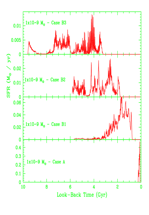
Figure 2: The SFR history in the four galaxy models with different mean initial density as a function of the look-back time in Gyr. The SFR is given in $M_{\odot}$/year. The initial density decreases from the bottom to the top panels (cf. Table 2 ).

Figure 3: Metal enrichment of the three model galaxies of type B as a function of the look-back time. The filled square along each curve shows the mean metallicity weighted on the star formation rate.

3 The Model Galaxies

The relevant data characterizing the final state of evolution of the four galaxies are summarized in Table 3. These are the mass in stars, the mass of remaining gas, the present-day effective radius of the baryonic matter $R_{e,B}$, the central velocity dispersions of baryonic and dark matter, $\sigma_{b}$ and $\sigma_{D}$ respectively, and an estimate of the maximum and mean metallicity weighted on the star formation rate $\Psi(t)$, $\log(Z/Z_{\odot})_{Max}$ and $\langle\log(Z/Z_{\odot})\rangle_{\Psi}$, respectively. In the discussion below particular attention is given to models of type B because they present the largest variety of SFHs. The results for the case A galaxies are very similar to those of case B1.

3.1 Star Formation and Metal Enrichment

Inside the virialized halo of DM, gas cools and sinks toward the center of the gravitational potential well, and sooner or later forms stars according to the adopted prescription.

The four panels of Fig. 2 show the SFR of our galaxies as a function of time. In model A with the highest initial density the SFR reduces to a prominent, initial burst of activity followed by quiescence. All the action is within a narrow age range of about 0.2 Gyr.

Passing to type B models the situation is more complex. Model B1 despite its significantly lower initial density compared to case A, still resembles this latter because the star forming activity is confined in the past. However, two important new features appear: first star formation is delayed for about 1 Gyr and second it stretches over an age range of about 3 Gyr. The SFR is somewhat irregular and intermittent. Moving to even lower initial densities (models B2 and B3) the features in question are amplified, the SFR shows indeed many burst-like episodes of short duration (shorter than 0.1-0.2 Gyr) superimposed on a gentle, nearly periodic trend with typical time scale of about 1 Gyr. This behavior is natural in small size galaxies (Hirashita et al. 2000) and is the consequence of the balance between cooling and heating as a function of the depth of the potential well. More preciseley, the rate of star formation and heating in turn scale with the density, whereas the cooling rate scales with the square of the density. Therefore, in a high density environment not only more stars are made and more energy and metals are injected but also cooling is more efficient so that it easier for the gas to meet the star formation condition. Star formation is somehow forced to completion. In contrast, in a low density medium, the rate of star formation and energy and metals injection tend to be lower, but also cooling becomes less efficient. The gas particles find it more difficult to meet the conditions required for star formation. As a consequence of it, the star forming activity become fluctuating and even discontinuous.

In the course of evolution, the galaxies convert their initial gas content into stars at different efficiencies. In general, the higher the mean initial density, the larger is the fraction of gas converted into stars. However, this trend can be counteracted by the effects of heating by supernova explosions, stellar winds etc. which in the case of very high efficiency such as in our case A may even lead to a lower fraction of gas being converted into stars (see the entries of Table 3 to be described below).

In all cases under consideration, the gas left over by the star forming process is partly lost (out of the virial radius) and partly locked in the outer DM halo. Finally the left-over gas is partly enriched (30$\%$) and partly unprocessed (70$\%$) because of the partial diffusive mixing.

In Fig. 3 we show the history of metal enrichment for the models B1, B2 and B3. Model A is not displayed here because thanks to the very initial spike of stellar activity and quiescence ever since, the metallicity is practically constant with time. In all other models we notice a continuous but irregular increase, characterized by some pauses and several jumps, which mark successive bursts of star formation. The maximum metallicity goes from $\log(Z/Z_{\odot})_{Max}$=-1.032 (B3) to $\log(Z/Z_{\odot})_{Max}$=-0.128 (B1) and $\log(Z/Z_{\odot})_{Max}$=-0.017 for model A. However, the mean metallicity weighted on the star formation rate $\langle\log(Z/Z_{\odot})\rangle_{\Psi}$ is much lower. It varies from $\langle\log(Z/Z_{\odot})\rangle_{\Psi}$=-1.48 (B3) to $\langle\log(Z/Z_{\odot})\rangle_{\Psi}$=-0.577 (B1) and $\langle\log(Z/Z_{\odot})\rangle_{\Psi}$=-1.158 (A).

It is worth commenting here that these values of the metallicity are merely indicative of the real situation owing to our over-simplified treatment of chemical enrichment.

Figure 4: The final distribution of the star density (in g cm^-3) in model B2. Superimposed is a Hernquist profile for the effective radius $R_{e,B}$ = 1.55 kpc.

Figure 5: Final radial distribution of the gas (solid line), stars (dotted line) and DM (dashed line) densities (in g cm^-3) in the model galaxies B1 and B3.

Figure 6: Iso-density contours of the gas distribution in model B2 as seen at the end of the simulation. The X and Y-axis are the spatial coordinates in kpc centered on the center of the gravitational potential. Note the circular annulus void of gas surrounding the central body of the galaxy. The gas in the outermost region is beyond the virial radius and therefore escaping from the galaxy (galactic wind).

Figure 7: Present-day gas and velocity profiles in the model galaxy B2. Upper Panel: The fractionary mass distribution of gas as function of the radial distance in kpc. Bottom panel: the radial velocity component $V_{r}(r)$ (dots) and the escape velocity $V_{esc}(r)$ (long dashed line) as a function of the galacto-centric distance. The vertical dashed line is the virial radius, whereas the vertical solid lines show the effective radius of baryonic matter, $R_{e,B}$ and the layer, $r_{esc}$, at which $V_{r}(r)>V_{esc}$. All the gas located at $r>r_{esc}$ freely flows out.

3.2 Final structure of the model galaxies

To illustrate how the mass of three main components, i.e. DM, gas and stars, is distributed in our model galaxies as a function of the radial distance, in Fig. 5 we show the present-day radial profiles of the mass density in gas (solid line), stars (dotted line), and DM (dashed line) limited to the cases of models B1 and B3.

3.2.1 Dark Matter

In our simulations, the DM halo surrounding the stellar and gaseous matter does not significantly change its properties in the course of evolution. The density profile of DM is very smooth, and depending on the initial conditions its central value ranges from a few $10^{-25}$ g/cm³ to a few $10^{-23}$ g/cm³. The most important result is that the innermost regions of the galaxies (within about 1 kpc of the center ) are dominated by baryons, whereas the outer parts are dominated by DM (see Fig. 5). Moreover, the velocity dispersion of the DM is about twice the velocity dispersion of the stars. These results agree with the notion that present-day DGs are DM-dominated (Salucci & Persic 1998), because the original content of baryonic material has been largely lost in galactic winds (see below).

3.2.2 Stars

The final stellar mass of the models is $3.2\times 10^{7}\,M_{\odot}$ for case A and it ranges from $1.3\times 10^{7}M_{\odot}$ to about $5.5\times 10^{7}M_{\odot}$ going from B1 to B3. The stellar component always dominates in the innermost regions of the galaxy models. In order to check whether our models may resemble real dwarf galaxies, the dwarf spheroidals in particular, we look closely at the model B2. At the end of the simulation the central density of stars is about $3\times 10^{-24}$ g/cm³ and the stellar matter occupies a central sphere of about 5 kpc radius (see Fig. 4), which is about five times smaller than the initial virial radius, even though the density gradient is so steep that most of the stellar mass is within the effective radius $R_{e,B}$. The spherically averaged stellar density profile of the same model is then compared with the Hernquist (1990) profile for the stellar distribution in a dwarf spheroidal with effective radius $R_{e,B}$ = 1.55 kpc (see Fig. 4). The remarkable agreement between the two profiles shows that the final galaxy resembles indeed a dwarf spheroidal. The effective radius of the model is about 17 times less than its initial virial radius. Finally, we like to note that as for kinematics the stellar velocity dispersion in the center of our model galaxies ranges from 10 to 3 km/s passing from case A to cases B1, B2 and B3 (see Table 3).

3.2.3 Gas

Most of the initial gas originally inside the DM halo is not processed into stars (see the entries of Table 3).

As expected in all models but for minor differences the spatial distribution of the gas in the central region closely follows the distribution of the stellar content (see Fig. 5).

However, there is an interesting feature to note looking at the large scale distribution of gas. The case is illustrated in Fig. 6 for the proto-type model B2. Of the gas left over inside the DM halo, only the fraction located in the central region keeps the original spatial distribution. The remaining part, heated up by the energy feed-back from supernova explosions and stellar winds, reaches regions very far from the central sphere containing most of the stars (i.e. the luminous part of the galaxy).

Finally, it is worth noticing that between the central part and the most distant regions there is a very low density, almost spherical shell, which is due to the strong galactic wind episode occurred in the past. This gas distribution resembles indeed the distribution of cold gas recently discovered by Blitz & Robishaw (2000) in a sample of dwarf spheroidal galaxies of the Local Group.

The major question is to be addressed whether or not part of the left over gas becomes gravitationally unbound to the main body of the galaxy thus freely escaping as galactic wind.

Table 4: Galactic winds.

$Model$	$M_{g}$	$R_{e,B}$	$R_{200}$	$M_{g,esc}$	$\Delta M_{g,w}$	${\Delta M_{g,w}\over M_{g}}$
	$10^{7}M_{\odot}$	kpc	kpc	$10^{7}M_{\odot}$	$10^{7}M_{\odot}$	%
A	6.8	0.07	4	2.4	4.5	66
B1	2.3	0.24	16	1.5	0.8	35
B2	7.5	1.55	26	5.2	2.3	30
B3	8.7	8.70	35	6.4	2.1	24

3.2.4 Galactic winds

The answer to the above question is given by Fig. 7, which displays the case of model B2, and Table 4, which lists the relevant data for all the models.

The top panel of Fig. 7 shows the fractionary gas content as a function of the radial distance in kpc, whereas the bottom panel shows the radial component of the gas velocity $V_{r}(r)$ (dots) and the escape velocity $V_{esc}(r)$ (long dashed lines) as a function of the galacto-centric distance. The vertical, dashed line is the initial radius $R_{200}$, whereas the vertical solid lines labelled $R_{eB}$ and $V_{r}>V_{esc}$ show the effective radius of BM and the layer at which $V_{r}>V_{esc}$.

There is a layer $R_{esc}$ at which the condition $V_{r}>V_{esc}$ is met. All the gas lying above it can freely leave the galaxy in form of galactic wind. However, the amounts of gas lost in the wind varies with the type of model i.e. the initial density. The situation is summarized in Table 4 which lists the model identification label, the total among of left-over gas $M_{g}$, the effective radius of BM $R_{e,B}$, the initial virial radius $R_{200}$, the gas content $M_{g,esc}$ up to at the layer at which the velocity equals the escape velocity, the amount of gas lost in the wind $\Delta M_{g,w}$, and the percentage of gas lost in the wind with the respect to the total available gas, ${\Delta M_{g,w}\over M_{g}}$.

In model A, the gas mass blown away in the galactic wind amounts to about 66% of the remaining gas, whereas in models of type B it is roughly a factor of two less.

There is a final remark to be made: within the effective radius of BM, very little gas remains. This is nearly zero for model A, it amounts to $\simeq 5\%$ for model B1, to $\simeq 15\%$ for model B2, and $\simeq 20\%$ for model B3. If our case A can be taken as representative of dwarf spheroidal galaxies, this would be consistent with the observed lack of gas in these systems (Mateo 1998). In contrast the reltively higher gas content in models B could make them more suited to interpret dwarf irregulars (case B3) or dwarf spheroidals/irregulars (cases B1 and/or B2) that seem to be gas-rich (Mateo 1998),

Table 5: $T_{G}$ is the present age (in Gyr) of the Galaxy models. $T_{U,z{for}}$ is the age of the Universe at the epoch of galaxy formation. $H_{0}$ is the Hubble constant in km/s/Mpc, whereas $q_{0}$ is the deceleration parameter. Finally $z_{for}$ is the red-shift at which galaxies are assumed to form.

$H_{0}$	$q_{0}$	$z_{for}$	$T_{G}$	$T_{U,z_{for}}$
50	0.	5	16.450	3.290
50	0.5	5	12.265	0.895
60	0.	5	13.708	2.742
60	0.5	5	10.220	0.746
70	0.	5	11.750	2.350
70	0.5	5	8.760	0.640

Figure 8: A simulated CMD according to the SFR of case A presented in Fig. 2. The mean metallicity is $\langle\log(Z/Z_{\odot})\rangle_{\Psi}$=-1.158. The left panel is for $H_{0}$=70, $q_{0}$=0.5, $z_{for}$=5, $T_{G}$=8.76 Gyr and $T_{U,z_{for}}$=0.64 Gyr. The right panel is the same but for $H_{0}$=50, $q_{0}$=0, $z_{for}$=5, $T_{G}$=16.45 Gyr and $T_{U,z_{for}}$= 3.29 Gyr. Finally, $1\sigma$ photometric errors are displayed at the right side of each panel.

Figure 9: The same as in 8, but for case B1. The mean metallicity is $\langle\log(Z/Z_{\odot})\rangle_{\Psi}$=-0.577. The left panel is for $H_{0}$=70, $q_{0}$=0.5, $z_{for}$=5, $T_{G}$=8.76 Gyr and $T_{U,z_{for}}$=0.64 Gyr. The right panel is the same but for $H_{0}$=50, $q_{0}$=0, $z_{for}$=5, $T_{G}$=16.45 Gyr and $T_{U_{for}}$= 3.29 Gyr.

Figure 10: The same as in 8, but for case B2. The mean metallicity is $\langle\log(Z/Z_{\odot})\rangle_{\Psi}$=-1.079. The left panel is for $H_{0}$=70, $q_{0}$=0.5, $z_{for}$=5, $T_{G}$=8.76 Gyr and $T_{U,z_{for}}$=0.64 Gyr. The right panel is the same but for $H_{0}$=50, $q_{0}$=0, $z_{for}$=5, $T_{G}$=16.45 Gyr and $T_{U,z_{for}}$= 3.29 Gyr.

Figure 11: The same as in 8, but for case B3. The mean metallicity is $\langle\log(Z/Z_{\odot})\rangle_{\Psi}$=-1.408. The left panel is for $H_{0}$=70, $q_{0}$=0.5, $z_{for}$=5, $T_{G}$=8.76 Gyr and is $T_{U,z_{for}}$=0.64 Gyr. The right panel is the same but for $H_{0}$=50, $q_{0}$=0, $z_{for}$=5, $T_{G}$=16.45 Gyr and $T_{U,z_{for}}$= 3.29 Gyr.

4 Color-Magnitude Diagrams

The aim of this section is to check whether the SFR and enrichment law of our model galaxies may generate CMDs like those observed today in dwarf galaxies of the Local Group.

Prior to this, one has to choose the link between the red-shift of galaxy formation, $z_{for}$ and age in order to convert the rest-frame ages used so far into absolute ages of the stars which would now be observed. This means that a certain model for the Universe has to be adopted. For the purposes of the present study we adopt the Friedman model described by the Hubble constant $H_{0}$ and deceleration parameter $q_{0}$. In all simulations we assume the same red-shift of galaxy formation, i.e. $z_{for}=5$. To facilitate the use of the simulations below, in Table 5 we summarize the maximum ages $T_{G}$ of the galaxy models, and the age $T_{U,z_{for}}$ of the Universe at $z_{for}=5$, for three different values of $H_{0}$ (50, 60 and 70 km/s/Mpc), and two values of $q_{0}$ (0 and 0.5). Higher values of both quantities are not likely here because they would predict galactic ages $T_{G}$ that are too old, at least compared to what is currently known about the age of globular clusters, i.e. from 10.0 to 15.8 Gyr as recently reviewed by Carretta et al. (2000).

Synthetic CMDs are constructed by means of a population synthesis algorithm. Given the galaxy age $T_{G}$, for each value of the stellar age $t$, an isochrone with the mean metallicity $\langle Z\rangle$ is derived from a set of stellar evolutionary tracks. These are from Girardi et al. (2000) for $0.0004\leq Z\leq 0.03$, and Girardi et al. (1996) for $Z=0.0001$. The evolutionary sequences span the mass and age ranges of $0.15\,M_{\odot}\leq M\leq 7\,M_{\odot}$, and from 0.06 to 20 Gyr. The mass and age ranges are fully adequate to describe the stellar populations of dwarf spheroidal galaxies. All important evolutionary phases are included, from the zero-age main sequence to the end of the thermally-pulsing asymptotic giant branch. The isochrones in the theoretical plane (luminosity versus effective temperature) are transformed to the observational magnitudes and colors using the transformations provided by Bertelli et al. (1994).

Each isochrone of age $t$ is populated by stars according to the Salpeter initial mass function (IMF), and in proportions fixed by the star formation rate, SFR$(T_{G}-t)$. The relative number of stars predicted in each section of the CMD is added to the composite population. The procedure continues for all values of the age, i.e. from the present ($t=0$) up to the maximum galaxy age ($t=T_{G}$).

Finally, the CMD is populated using a arbitrary total number of stars. In the present simulations, we include the effects of photometric errors and neglect those of binaries for the sake of simplicity. Photometric errors are assumed to be similar to those obtained by Smecker-Hane & McWilliam (1999) in HST observations of Carina dSph.

The most uncertain ingredient of these CMD simulations is mass loss along the red giant branch (RGB) of low-mass stars. This is taken into account by decreasing the stellar mass when passing from the tip of the RGB to the zero-age horizontal branch (see Renzini 1977). Mass loss is assumed to follow the Reimers (1975) law with a suitable value of the parameter $\eta$ (Fusi-Pecci & Renzini 1976). It is worth recalling that by applying mass loss at the stage of isochrone construction (and not during the computation of evolutionary tracks) allows us to easily vary $\eta$ from simulation to simulation if required. We adopt the mean value $\langle\eta\rangle=0.50$ with dispersion $\sigma_{\eta}=0.05$. These values are slightly larger that those used to reproduce the morphology of globular clusters (Renzini & Fusi-Pecci (1988) but still within current uncertainties.

The above technique is used to generate the CMDs shown in Figs. 8 through 11 for the SFHs (Fig. 2) and the enrichment rate (Fig 3) of our model galaxies A, B1, B2, and B3. Furthermore, CMDs are presented for two, somewhat extreme values of the galaxy age $T_{G}$ corresponding to different values of $H_{0}$, $q_{0}$, $z_{for}$, $T_{U,z{for}}$ as indicated.

Model A. Case A is straightforward because owing to its prominent and unique initial burst of activity, the associated CMD would simply resemble that of a globular cluster. This is shown in the two panels of Fig.8. The left panel is for $H_{0}$=70, $q_{0}$=0.5, $z_{for}$=5 and $T_{G}$=8.76 Gyr, whereas the right panel is for $H_{0}$=50, $q_{0}$=0, $z_{for}$=5, and $T_{G}$=16.45 Gyr. The two panels clearly show how the CMD of a globular cluster with intermediate mean metallicity ($\langle\log Z/Z_{\odot}\rangle_{\Psi}$=-1.158) changes as a function of the age. Passing from the young (left) to the old (right) population, the turn-off luminosity decreases whereas the clump of red stars (He-burners) turns into an extended horizontal branch. This is more populated at the red side because the metallicity is somewhat higher than the typical value in globular clusters with very extended horizontal branches, mostly populated at the blue side.

Model B1. The left and right panels of Fig.9 show the expected CMD for the models B1. The CMD of the older age (right panel) much resembles the one of an old globular cluster with relatively high metallicity, $\langle\log Z/Z_{\odot}\rangle_{\Psi}$=-0.577 according to the entries of Table 3. There is some blurring at the turn-off and sub-giant branch due to the large age spread caused by the prolonged initial stellar activity (about 3 Gyr). These effect adds a new dimension to the horizontal branch, because it is now populated by stars with significantly different initial mass, which tends to evenly populate the horizontal branch. Despite the high metallicity, this CMD could closely mimic the ones of Sculptor (see Fig. 1) or Ursa Minor and Draco, i.e. galaxies dominated by a single burst of SF which extended for some time (see Hernandez et al. 2000). By decreasing the age down to 9 Gyr, the red clump (typical of an intermediate age population) appears. Although the star formation lasted for about 3 Gyr, its ever decreasing efficiency past the initial peak does not allow the presence of a secondary distinct generation of stars but only a large scatter at the turn-off. This CMD is a good candidate to explain the properties of Leo II (Hernandez et al. 2000).

Model B2. The panels of Fig.10 show the expected CMD for the same value of $z_{for}$, $H_{0}$ and $q_{0}$=0 as in Figs. 8 and 9 but for model B2. The CMD of the right panel does not significantly differ from its analog in Fig. 9 but for a larger scatter at the turn-off, sub-giant branch, and horizontal branch. The CMD in the left panel owing to its much younger age clearly shows the several distinct bursts of star formation already noticed in Fig. 2.

Model B3. Finally we have the case of models B3, whose CMD is shown in the left and right panels of 11 for the same combinations of $H_{0}$, $q_{0}$ and $z_{for}$ as in the previous simulations. The results of the right panel ($H_{0}$=50, $q_{0}$=0, $T_{G}=16.45$ Gyr) are particularly interesting because three distinct old populations are now visible going from old to relatively young (say about 6 Gyr). Galaxies like Leo I or Carina could be reproduced by a star formation history like this. See for instance the CMD of Fig. 1 for Carina, or that of Leo I given by Held et al. (2000). The CMD of the left panel, owing to the much younger ages involved and almost continuous star formation up to the present could perhaps mimic the case of a DIrr.

A general remark. The above simulations of dwarf galaxies and associated CMDs were not designed to match any particular dwarf galaxy. In most cases, the metallicity of the models was too high compared to observational value. This is certainly due to the adoption of the closed-box description. Work is in progress to improve upon the treatment of chemical enrichment. Our simulations are intended only to show that dwarf galaxies with the same total mass of $10^{9}M_{\odot}$ but originated from proto-galaxies of different initial densities may undergo different histories of star formation which in turn yield different CMDs, in agreement with the large variety of observational data for such galaxies. Dwarf galaxies formed in a high density environment tend to have a single initial burst of stellar activity. In contrast, galaxies of the same mass but with low initial density tend to undergo star formation over long periods of time, showing a number of burst-like episodes. In some extreme cases star formation may stretch up to the present. Accordingly we pass from galaxies that would nowadays appear as DSph, DE and DIrr.

5 Summary and conclusions

We have tried to understand the physical reason for the large variety of star formation histories indicated by the stellar content of dwarf galaxies, with particular attention to the case of dwarf spheroidals and ellipticals. Indeed objects whose estimated mass in stars, mean metallicity, and velocity dispersion span a rather narrow range of values, can have very different star formation histories.

With the aid of Tree-SPH, N-Body simulations of galaxy formation and evolution we find that systems of the same total (dark and baryonic) mass but different initial densities may have different star formation histories ranging from a single initial episode to prolonged stellar activity extended into a series of bursts over a large fraction of the Hubble time.

Starting from ”realistic” initial conditions, we follow the monolithic collapse of baryons inside the virialized halo of DM, and the formation of stars by gas cooling and collapse. The models include accurate treatments of star formation, chemical enrichment, energy feed-back from supernova explosions and stellar winds, and metal-dependent cooling.

The structural properties of the models remarkably agree with the observational data of real galaxies (mass density profiles, central velocity dispersions, mean metallicities, mass-to light ratios, and even gas distributions).

Furthermore, using the theoretical star formation and metal enrichment histories of the model galaxies we simulate the CMDs that one would expect to observe today as a function of the underlying cosmological parameters $H_{0}$, $q_{0}$, $z_{for}$ and $T_{G}$. In many cases the simulated CMDs remarkably resemble the observational ones.

The main conclusion of this study is that the adopted scheme of galaxy formation, i.e. early virialization of DM haloes and monolithic collapse of baryons into their potential wells, may lead to a variety of different situations as far as the detailed star formation histories is concerned, that depend on the initial density of the system.

Together with the results of the companion paper by Carraro et al. (2001), briefly summarized in Section 2, this study suggests that total mass and initial density are the key parameters governing the final stellar content of elliptical galaxies. Ample possibilities exist for star formation histories, ranging from a single initial episode of short duration, to large time intervals, to burst-like activities, and even to very prolonged star formation.

A final consideration is worth being made here. Throughout the analysis, when referring to the initial density this has been linked to red-shift via the over-density with respect to the mean density of the Universe required by a proto-galaxy to detach himself from the Hubble flow and to collapse. This indeed was the over-density assigned to model A. Strictly speaking, at the red-shift of galaxy formation we have considered only models of type A are possible. To have models of type B brought into existence one has to wait for a fall-off of the over-density by a factor of 70 at least, or equivalently $\Delta z_{for}\simeq 3$. In other words, galaxies of similar mass but formed at $z_{for}\simeq 2$ would behave as models B and for $50\leq H_{0}\leq 60$ and $q_{0}\simeq 0$ would have a maximum age for their stellar populations still fully compatible with the information derived from the observational CMDs. In other words, proto-galaxies of the same total mass collapsing at different red-shifts would contain different kinds of stellar populations.

References

- [1] Barnes J.E., Hut P., 1986, Nature, 324, 446
- [2] Bertelli G., Bressan A., Chiosi C., Fagotto F., Nasi E., 1994, A&AS, 106, 275
- [3] Binney J., Tremaine S., 1987, Galactic Dynamics, Princeton University Press, Princeton, New Jersey, USA
- [4] Blitz L., Robishaw T., 2000, ApJ, 541, 675
- [5] Bressan A., Chiosi C., Fagotto F., 1994, ApJS, 94, 63
- [6] Buonomo F., Carraro G., Chiosi C., Lia C., 2000, MNRAS, 312, 371
- [7] Carraro G., Lia C., Chiosi C., 1998, MNRAS, 298, 1021
- [8] Carraro G., Lia C., Chiosi C., 2001, MNRAS, to be submitted
- [9] Carretta E., Gratton R., Clementini G., Fusi-Pecci F., 2000, ApJ, 533, 215
- [10] Chiosi C., Maeder A., 1986, ARA&A, 24, 329
- [11] Chiosi C., Bressan A., Portinari L., Tantalo R., 1998, A&A, 339, 355
- [12] Fusi-Pecci F., Renzini A., 1976, A&A, 46, 447
- [13] Gallart C., Freedman W.L., Aparicio A., Bertelli G., Chiosi C., 1999, AJ, 118, 2245
- [14] Gingold R.A., Monaghan J.J., 1977, MNRAS, 181, 375
- [15] Girardi L., Bressan A., Chiosi C., Bertelli G., Nasi E., 1996, A&AS, 117, 113
- [16] Girardi L., Bressan A., Bertelli G., Chiosi C., 2000, A&AS, 141, 371
- [17] Greggio L., Renzini A., 1983, A&A, 118, 217
- [18] Groom W., 1997, PhD Thesis, Cambridge University
- [19] Held E.V., Saviane I., Momamy Y., Carraro G., 2000, ApJ, 530, L85
- [20] Hernandez X., Gilmore G., Valls-Gabaud D., 2000, MNRAS 317, 831
- [21] Hernquist L., 1990, ApJ, 356, 359
- [22] Hirashita H., 2000, PASJ, 52, 107
- [23] Hollenback D., McKee C.F., 1979, ApJS, 41, 555
- [24] Lacey C., Cole S., 1993, MNRAS, 262, 627
- [25] Lacey C., Cole S., 1994, MNRAS, 271, 676
- [26] Larson R.B., 1974, MNRAS, 166, 585
- [27] Lucy L., 1977, AJ, 82, 1013
- [28] Mateo M., 1998, ARA&A, 36, 435
- [29] Portinari L., Bressan A., Chiosi C., 1998, A&A, 334, 505
- [30] Reimers D., 1975, Mem. Soc. R. Sci. Liege, ser. 6, vol. 8, p. 369
- [31] Renzini A., 1977, in Advanced Stages of Stellar Evolution, eds. P. Bouvier and A. Maeder, Geneva Observatory, p. 151
- [32] Renzini A., Fusi-Pecci F., 1988, ARA&A, 26, 199
- [33] Salpeter E.E., 1955, ApJ 121, 161
- [34] Salucci P., Persic M., 1998, in ”Dark and Luminous Matter in Galaxies”, ASP Conf. Ser. Vol. 117, p.1
- [35] Smecker-Hane T., McWilliam A., 1999, ”Spectro-photometric dating of stars and galaxies” eds. I. Hubney, S. R. Heap, R. H. Cornett, ASP Conf. Ser. Vol. 192, 251
- [36] Sutherland R. S., Dopita M. A., 1993, ApJS, 88, 253
- [37] Tinsley B.M., 1980, Fundamentals of Cosmic Physics 5, 287
- [38] Thornton K., Gaudlitz M., Janka H.-Th., Steinmetz M., 1998, ApJ, 500, 95
- [39] White S.D.M., Rees M.J., 1978, MNRAS, 183, 341