Statistical Properties of Galactic Starlight Polarization

Abstract

We present a statistical analysis of Galactic interstellar polarization from the largest compilation available of starlight data. The data comprises $\sim 9300$ stars of which we have selected $\sim 5500$ for our analysis. We find a nearly linear growth of mean polarization degree with extinction. The amplitude of this correlation shows that interstellar grains are not fully aligned with the Galactic magnetic field, which can be interpreted as the effect of a large random component of the field. In agreement with earlier studies of more limited scope, we estimate the ratio of the uniform to the random plane-of-the-sky components of the magnetic field to be ${\bf B_{u}/B_{r}}\approx 0.8$. Moreover, a clear correlation exists between polarization degree and polarization angle what provides evidence that the magnetic field geometry follows Galactic structures on large-scales.

The angular power spectrum $C_{\ell}$ of the starlight polarization degree for Galactic plane data ($|{\rm b}|<10^{\circ}$) is consistent with a power-law, $C_{\ell}\propto\ell^{-1.5}$ (where $\ell\approx 180^{\circ}/\theta$ is the multipole order), for all angular scales $\theta\mathrel{\hbox to0.0pt{\lower 3.0pt\hbox{$\mathchar 536\relax$}\hss}\raise 2.0pt\hbox{$\mathchar 318\relax$}}10^{\prime}$. An investigation of sparse and inhomogeneous sampling of the data shows that the starlight data analyzed traces an underlying polarized continuum that has the same power spectrum slope, $C_{\ell}\propto\ell^{-1.5}$. Our findings suggest that starlight data can be safely used for the modeling of Galactic polarized continuum emission at other wavelengths.

1 Introduction

The large scale emission from the Milky Way at radio, mm-wave and far-infrared wavelengths is known to be polarized (see e.g, de Oliveira-Costa & Tegmark 1999). The underlying common cause is the Galactic magnetic field, though the particular polarization mechanism is wavelength-dependent. It ranges from the synchrotron emission process which is the driving mechanism at long wavelengths to the absorption/emission properties of aligned dust grains which are expected to account for the short-wavelength emission. Therefore the measurement of the polarized Galactic emission should yield valuable information on our Galaxy’s magnetic field (see e.g, Zweibel & Heiles 1997, Hildebrand et al 2000, Heitsch et al 2001). In particular, starlight polarization vectors trace the plane-of-the-sky projection of the Galactic magnetic field (Zweibel & Heiles 1997) and measurements of polarization for stars of different distances reveals the 3D distribution of magnetic field orientations averaged along the line of sight.

However currently the only available large scale maps of polarized Galactic emission are at low (radio) frequencies (i.e, $\nu\leq 2.7$ GHz, see Tucci et al 2000, for a description of available data), where the Galactic signature is significantly distorted by (relatively) local Faraday rotation effects. At far-infrared and mm wavelengths, measurements have been made of a few very small regions, largely dense dark clouds, mainly concentrated in the Galactic plane (Hildebrand et al 1999, Novak et al 2000; see also Hildebrand et al 2000, Heitsch et al 2001, for recent reviews) but they reflect only rather local distortions of the large-scale magnetic field. Therefore, within this wavelength range, the only large scale view has been obtained by observation of and analogy with external spiral galaxies similar to our own (Zweibel & Heiles 1997).

The next generation of Cosmic Microwave background (CMB) missions (i.e. MAP -
http://map.gsfc.nasa.gov/ - and Planck - http://astro.estec.esa.nl/Planck) will fill this gap by providing polarization measurements of the whole sky at mm wavelengths. For these missions, the polarized Galactic dust emission is primarily a nuisance which has to be removed from the underlying cosmic signal (see Prunet & Lazarian 1999, Draine & Lazarian 1999, Lazarian 2001), but in so doing they will also provide for the first time the means to map the Galactic magnetic field. Planck in particular covers a range of wavelengths (1 cm to 300 $\mu$m) in which different polarization mechanisms are dominant, which will provide powerful means to uncover the common underlying magnetic field distribution.

At optical wavelengths, there do exist many measurements of starlight polarization
(Appenzaller 1974, Schroeder 1976, Mathewson et al 1978, Markkanen 1979, Krautter 1980, Korhonen & Reiz 1986, Bel et al 1993, Leroy 1993, Berdyugin et al 1995, Reiz & Franco 1998). Observed starlight polarization is believed to be caused by selective absorption by magnetically aligned interstellar dust grains along the line of sight; because these measurements are limited by dust extinction, they give us a view of the behavior of the magnetic field only in a local bubble around us. Furthermore, the pencil-beam nature of these observations means that the view afforded is punctual, with a sampling that is both inhomogeneous and sparse. However, analysis of compilations of such measurements (see Heiles 2000 and references therein) imply that they do contain information about both the large-scale and the random components of the Galactic field in the vicinity of the Sun. Therefore it is useful to extract as much information as possible from this data.

In this paper we analyze the most complete compilation to date of optical polarization observations. This analysis will allow us to extract basic information on the large scale statistical properties of the polarization field in the visible. We do this by studying the correlations between stellar parameters and computing the angular power spectrum (a convenient statistical estimator for analyzing 2D full-sky maps) of the optical polarization degree from Milky Way stars; in so doing we investigate the systematic effects introduced by the sparse and inhomogeneous sampling which is intrinsic to starlight measurements.

The outline of the paper is as follows: §2 presents the starlight data analyzed. We describe the distribution of the sources in §3 and study their correlations as a function of distance and Galactic coordinate in §4. We compute the angular power spectrum of starlight polarization degree in §5. We finish with a discussion of our results in §6.

2 Data

The starlight polarization data used in this analysis is taken from the compilation by Heiles 2000. This compilation includes data from 9286 sources taken from a dozen of catalogs, combining multiple observations, providing accurate positions and reliable estimates for extinction and distance of stars.

From this catalog, we have selected a subsample of 5513 stars ($60\%$ of the data) based on the following criteria:

• the degree and angle of polarization are given

• small absolute error in the polarization degree ($<0.25\%$)

• a (positive) extinction is given

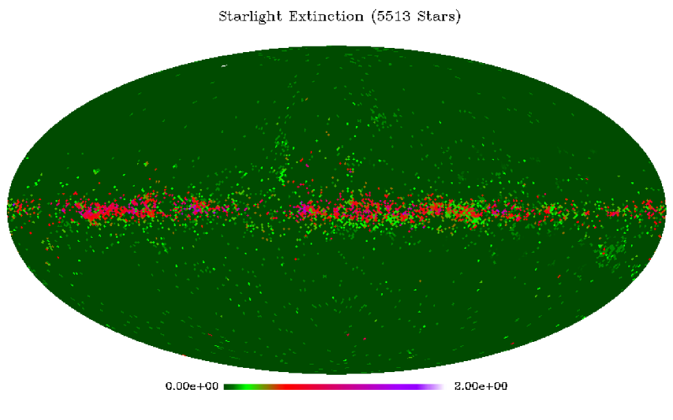
Note that the most constraining requirement is the last one (extinction): if this requirement were not used, the subsample would include 8280 stars (90 $\%$ of the whole compilation). However we need to include the degree of extinction in the visible as it strongly correlates with the polarization degree (see §4 below) and it is a basic ingredient to model dust polarization at other wavelengths (Hildebrand & Dragovan 1995). We shall present this analysis in a forthcoming paper (Fosalba et al 2001). All the stars in the Heiles compilation fulfilling the above requirements also have quoted distance (with an estimated 20 $\%$ error for most of the sources, see Heiles 2000).

3 Distribution of Sources

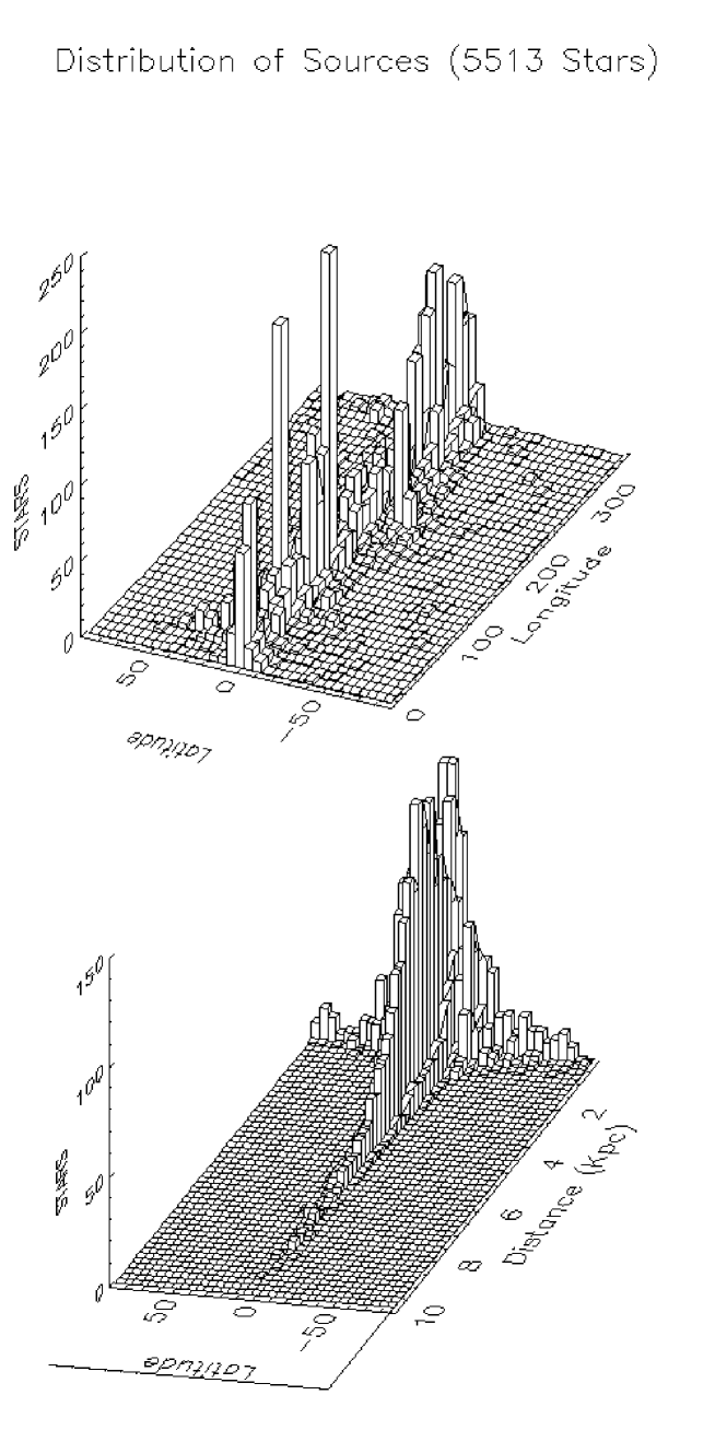
Fig 1 shows the distribution of sources in our subsample for data binned in Galactic coordinates (top panel) as well as in distance and latitude (bottom panel). As shown in the latter, all high latitude ($|{\rm b}|>10^{\circ}$) stars are nearby (d $<$ 1 Kpc). Within the Galactic plane one can find relatively distant stars, though the vast majority are within 2 Kpc. Thus, this is clearly a local sample.

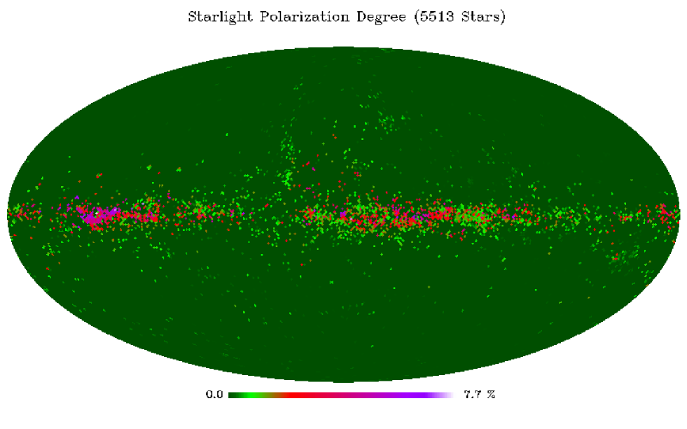
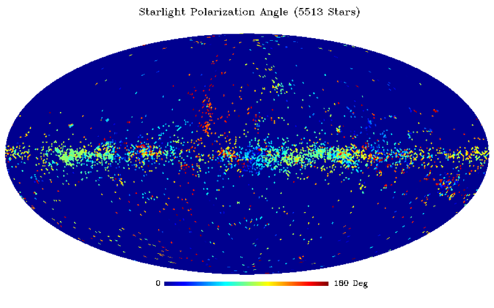
This is also seen in Table 1, which summarizes the mean stellar parameters (i.e, polarization degree P($\%$) and extinction as measured by the color excess E(B-V) ) in the subsample as a function of latitude and distance. Note that in Table 1, high latitude (low latitude) means $|{\rm b}|>10^{\circ}$ ($|{\rm b}|<10^{\circ}$) and nearby (distant) denotes d $<$ 1 Kpc (d $>$ 1 Kpc). The quantities between brackets denote amount $\%$ of all stars in the sample. Low-latitude stars have large values of the polarization degree P($\%$) $\approx 1.7$, and extinction E(B-V) $\approx 0.5$, while high-latitude sources exhibit significantly lower values, P($\%$) $\approx 0.5$, E(B-V) $\approx 0.15$. Polarization vectors (defined with respect to galactic coordinates) are typically oriented along the galactic plane ($\theta_{p}\approx 90^{\circ}$) although a more detailed analysis reveals a rich spatial distribution (see Fig 11 and §4 below).

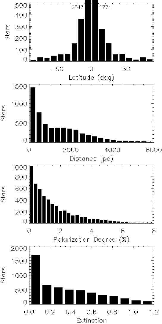
Histograms displaying the distribution of sources with Galactic latitude b, distance d, polarization degree P($\%$) and extinction E(B-V) bins, are given in Fig 2.

4 Correlations between Stellar Parameters

Light emitted from stars is assumed to be unpolarized; the observed polarization from starlight is believed to result from extinction by interstellar dust grains along the line of sight to the observer. Thus, for a homogeneous distribution of intervening dust, the larger the path-length starlight travels to reach the observer, the larger the polarization degree and extinction are expected to be. According to this simple picture, Galactic regions with low polarization degree (and extinction) trace nearby stars, while regions with high values of these parameters correspond to distant stars. This is actually observed in the sample of Starlight data, as shown in Figs 9 & 10, where nearby stars (light green sources) are mainly at high Galactic latitudes, while distant stars (red-purple sources) are found in the Galactic plane (see also Table 1 for mean values of the stellar parameters). In particular, the spatial distribution of both parameters in Galactic coordinates is expected to be highly correlated and this is clearly observed in Figs 9 & 10.

We describe in detail below how the stellar parameters which describe the sources in the subsample correlate with one another and what information can be extracted from the behavior found.

4.1 Behavior with Distance

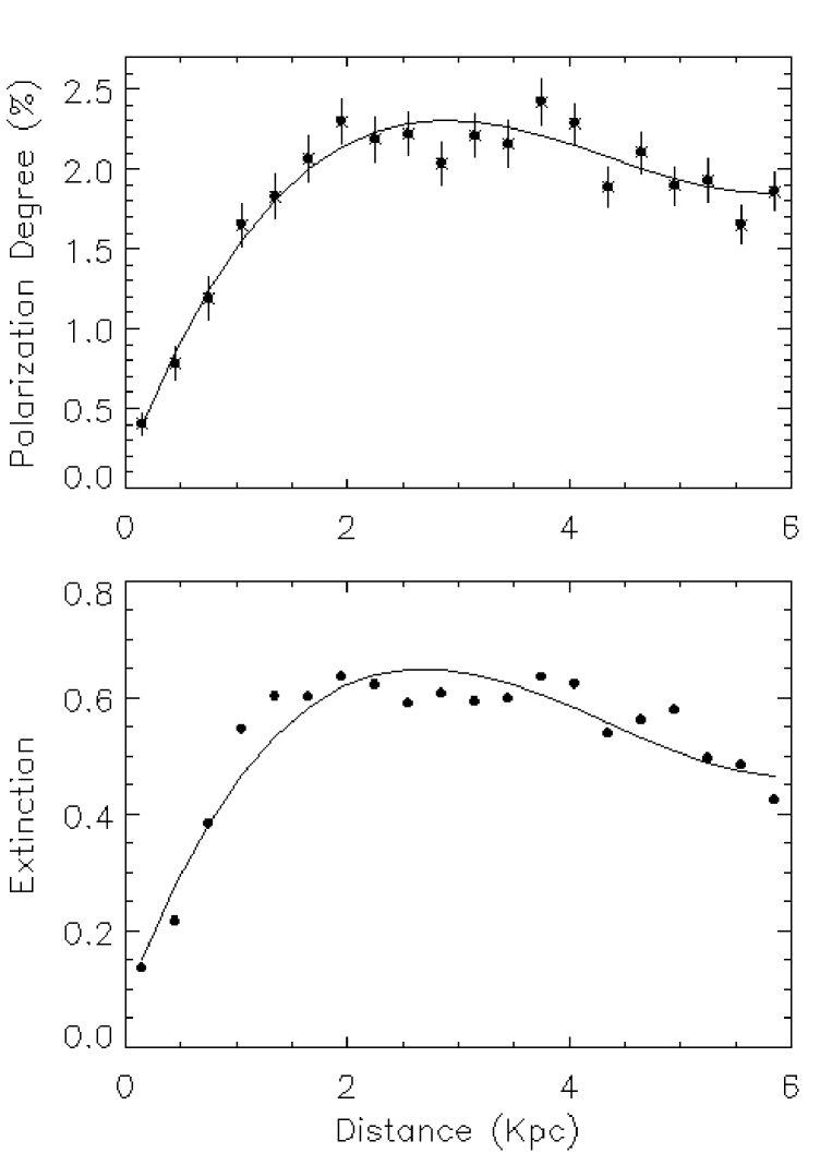
The distribution of the polarization degree and extinction as a function of distance (average quantities in linear distance bins) for the sources considered are shown in Fig 3. It is seen that both stellar parameters grow linearly (to a good approximation) with distance up to d $\approx 2$ Kpc. Beyond $\sim$2 Kpc, stars have roughly constant values for both quantities, i.e, P($\%$) $\approx$ 2, E(B-V) $\approx$ 0.6 . The overall behavior of P($\%$) and E(B-V) with distance (in Kpc) can be best-fitted by third-order polynomials up to d $\approx 6$ Kpc(see Fig 3):

$${\rm P}(\%)\approx 0.13+1.81\rm d-0.47\rm d^{2}+0.036\rm d^{3}~{},$$ (1)

$${\rm E(B-V)}\approx 0.08+0.5\rm d-0.135\rm d^{2}+0.0104\rm d^{3}~{}.$$ (2)

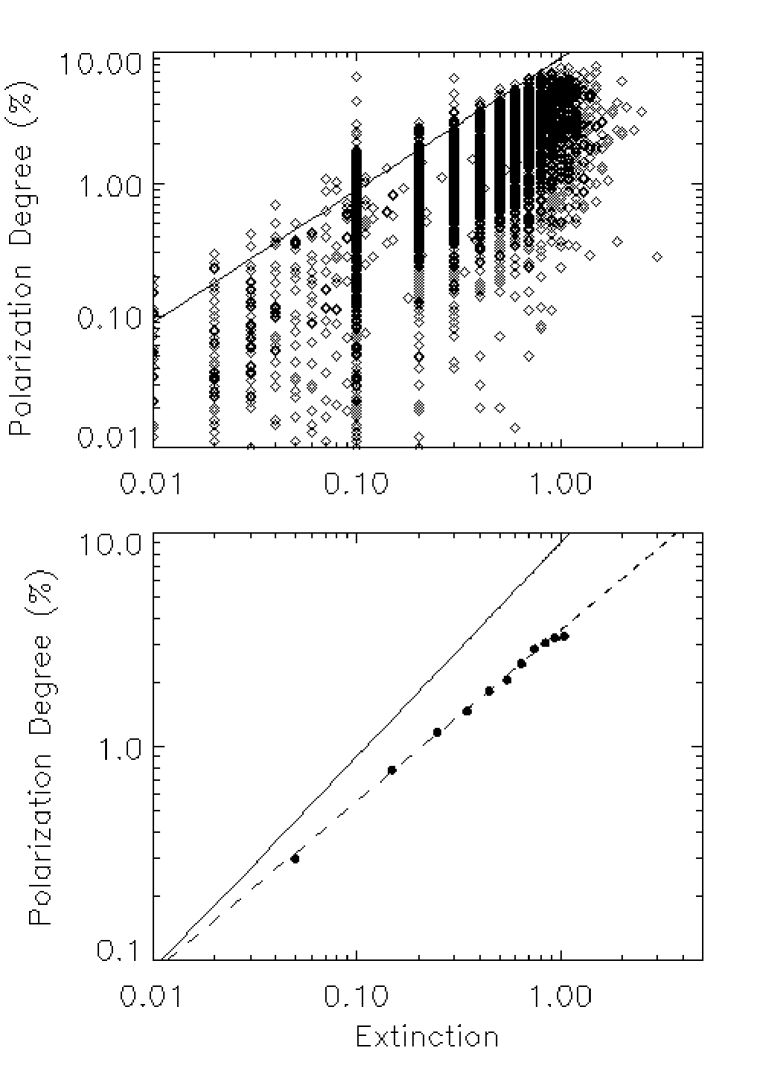
The similar behavior of both stellar parameters with distance already suggests a simple linear correlation (for data averaged in distance bins) between polarization degree and extinction. This is the case indeed as shown in Fig 4. The observed roughly linear correlation for individual sources is in agreement with measurements at 2.2 $\mu$m (Jones 1989) & 100 $\mu$m (Hildebrand et al 1995).

However the observed mean correlation amplitude for data averaged in extinction bins is much smaller than what is expected from interstellar dust grains completely aligned under a purely regular (no random component) external magnetic field P($\%$) $\approx$ 9 E(B-V). This is also observed in the K-filter at 2.2 $\mu$m (Jones 1989). What is more, we find a slight deviation from the simple linear correlation,

$${\rm P(\%)}\approx 3.5~{}{\rm E(B-V)}^{0.8},$$ (3)

as displayed in the lower panel of Fig 4. In fact, this deviation from the linear correlation shows a similar dependence with extinction for the K-band observations at 2.2 $\mu$m, i.e,
${\rm P_{k}}\approx$ 0.83 E(B-V)^0.75 (Jones 1989). Eq(3) implies that the ratio of the observed to the optimal polarization degree,

$${\rm{P_{Obs}\over P_{Max}}}\approx 0.39~{}{\rm{E(B-V)}}^{-0.2}$$ (4)

This is, at least, a factor of 2 larger than the same ratio found for the K-filter at 2.2 $\mu$m, ${\rm P_{Obs}/P_{Max}}\approx 0.19$ (Jones 1989). Next we study the dependence of the stellar parameters with Galactic coordinate.

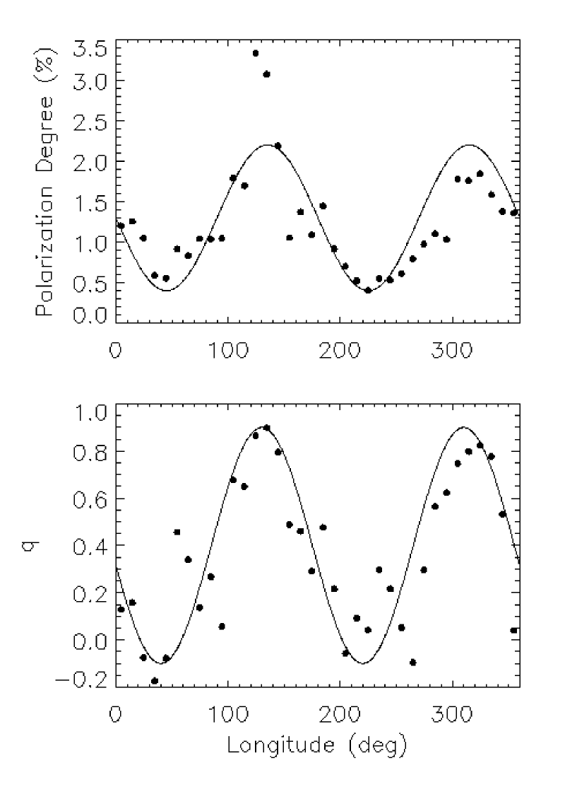
4.2 Behavior with Galactic Longitude

In order to study the dependence of stellar parameters with Galactic longitude we have averaged the data in 10^∘ longitude bins. As shown in Fig 5, both the polarization degree and the q parameter, defined as $q=\cos 2(\theta_{p}-90^{\circ})$ ($\theta_{p}$ is the polarization angle), exhibit, on average, a sinusoidal-like dependence with longitude with a 180^∘ periodicity, well-fitted by the expressions,

$${\rm P}(\%)\approx 1.3+0.9\sin(2\,l+180^{\circ})~{},$$ (5)

$${\rm q}\approx 0.4+0.5\sin(2\,l+190^{\circ})~{}.$$ (6)

For Galactic longitudes $l\approx 50^{\circ}$ and $l\approx 230^{\circ}$ we find minimum values of q, i.e, the stellar polarization vectors are orthogonal to the Galactic plane, $\theta_{p}\approx 0^{\circ},180^{\circ}$. Note that, at the Galactic plane, these directions approximately intersect the Cygnus-Orion spiral arm which suggests that, on average, polarization vectors do there not align with this Galactic structure. Moreover, we also find minimum values of the polarization degree (or extinction as they are nearly linearly correlated) for these Galactic longitudes. Approximately along these directions (as one moves away from the Galactic plane) one finds the edge of a supernova remnant, the spherical shell of Loop I (see red sources in Fig 11). Thus, a possible explanation for the values of the stellar parameters along these directions is that exploding supernovae in the Scorpius/Ophiuchus star cluster centered at $l\approx 0^{\circ}$, b $\approx 20^{\circ}$ (see Zweibel & Heiles 1997) could cause polarization vectors to be strongly aligned with the Galactic structure left by the supernova remnant.

On the other hand, maximum values of the polarization degree and q parameter are found at $l\approx 140^{\circ}$ and $l\approx 320^{\circ}$, where the polarization vectors of dust grains are parallel to the Galactic disk structure, $\theta_{p}\approx 90^{\circ}$ (see light-green sources in Fig 11).

We note that the results shown in the lower panel of Fig 5 for the longitude dependence of the q parameter are in good agreement with the analysis presented in Whittet (1992) for about 1000 nearby Galactic plane stars (d $<0.6~{}\rm{Kpc}$, $|{\rm b}|<3^{\circ}$).

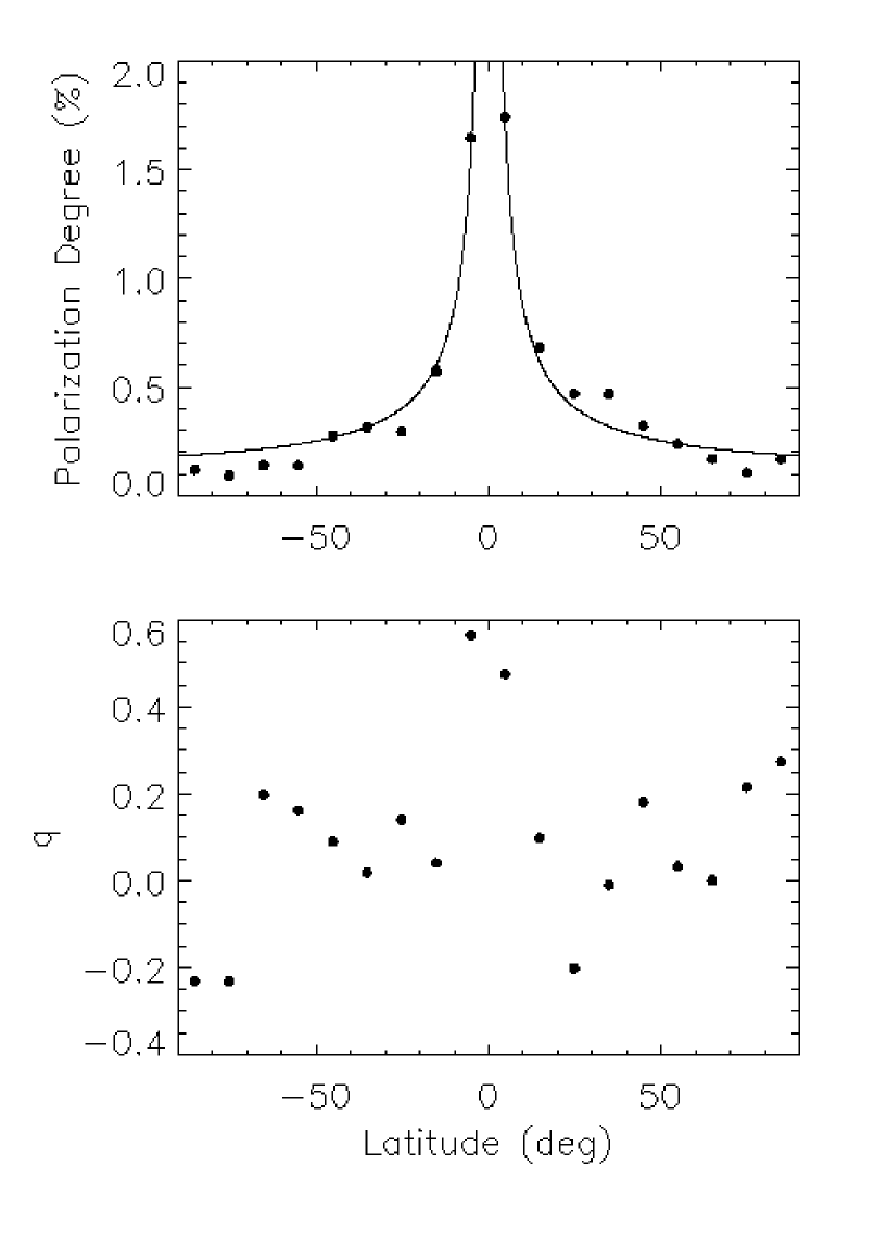
4.3 Behavior with Galactic Latitude

As discussed in §3, most of the sources in our subsample are in the Galactic disk (75 $\%$ of the stars are found at $|{\rm b}|<10^{\circ}$, see Table 1). However, there is a statistically significant fraction of the sources at high Galactic latitudes (25 $\%$ of sources at $|{\rm b}|>10^{\circ}$) which allow us to investigate the mean variation of the correlations between stellar parameters as a function of latitude. For this purpose we have averaged the data in $10^{\circ}$ (linear) latitude bins.

We find that the polarization degree shows a strong dependence with latitude as shown in the upper panel of Fig 6. Indeed, the behavior can be well described by a co-secant law:

$${\rm P}(\%)\approx 0.1+0.0067\csc(0.05~{}|{\rm b}|).$$ (7)

The statistical significance in the measurement of the q parameter (i.e, the polarization angle) is low at high latitudes given the lack of available data and the large degree of dispersion in the polarization angle (as large as 35-55 $\%$, depending on latitude and distance; see also the large scatter in lower panel of Fig 5). Therefore it is hard to draw any conclusions about the correlation between the polarization degree and q parameter on high Galactic latitudes from the current analysis.

5 The Angular Power Spectrum of the Starlight Polarization Degree

In this section, we analyze the starlight polarization data described in §2 to see whether and if so, to what extent, it traces from a statistical point of view the large-scale pattern of starlight polarization. By this we mean that ISM dust grains provide a discrete (and high-resolution) picture of the diffuse polarizing ISM along a few lines-of-sight, from which one aims at reconstructing (using in particular the power spectrum analysis presented below) the large-scale (low-resolution) statistical properties of the ISM polarization pattern.

In fact, the large-scale statistical properties of the ISM polarization from absortion of starlight by dust grains might give direct statistical information on the polarized diffuse emission by dust: if the grains that extinct starlight and emit constitute the same grain population, the power spectrum of starlight polarization degree is directly related to the power spectrum of polarized emission from dust.

Starlight polarization is caused by aligned grains with sizes $10^{-4}>a>10^{-5}$ cm (Kim & Martin 1995). These are essentially the grains responsible in diffuse media for polarized emission (see Prunet & Lazarian 1999). Therefore if aligned grains in diffuse medium have the same temperature the power spectrum of the starlight polarization should be identical to the spectrum of the polarized continuum from dust in the far infrared range (e.g, $100\mu$ m). The temperature difference between graphite and silicate grains will not change this result as graphite grains are usually not aligned (see Whittet 1992). In diffuse media, unlike in molecular clouds, the grains are exposed to a similar radiation flux and find themselves in a very similar physical environment. Therefore we do not expect substantial variations of the grain temperature and believe that the power spectrum we find will also represent the power spectrum of the polarized dust emission.

For this purpose we estimate the angular power spectrum (PS hereafter) of the starlight polarization degree (see Fig 9). The angular power spectrum is the convenient full-sky generalization of the 2D Fourier power spectrum, as the latter is only strictly valid in small (flat) patches of the sky. In particular, given a full-sky map of a scalar field S (such as the starlight polarization degree) one can decompose it into spherical harmonic basis, $Y_{\ell m}$, at any point ($\theta,\phi$) in the sky:

$$S(\theta,\phi)=\sum_{\ell m}a_{\ell m}Y_{\ell m}(\theta,\phi)\,.$$ (8)

The spherical harmonic basis, $Y_{\ell m}$, is the generalization of the Fourier basis to the sphere (as opposed to the usual flat space description). The $a_{\ell m}$’s are the amplitudes of the decomposition of a scalar field on this basis and they are assumed to be random Gaussian variables.

The angular power spectrum is thus defined as a quadratic average of a given $a_{\ell m}$ coefficient over different m-modes:

$$C_{\ell}={1\over{2\ell+1}}\sum_{m=-\ell}^{m=\ell}|a_{\ell m}|^{2}$$ (9)

where $C_{l}$ estimates autocorrelations of the field at an angular scale $\theta\approx 180^{\circ}/\ell$, being $\ell$ the so-called multipole order. In a fully-sampled map, the two-point correlation function $\xi(\theta)$ of the scalar field ${\rm S}$ is simply related to the angular power spectrum:

$$\xi(\theta)=<S({\bf q_{1}})S({\bf q_{2}})>=\sum_{\ell}{\ell+1/2\over{\ell(\ell+1)}}C_{\ell}P_{\ell}(\cos\theta)$$ (10)

where $\cos\theta={\bf q_{1}}\cdot{\bf q_{2}}$ is the dot product of two unit vectors pointing to any pair of sky pixels, $P_{\ell}$ is the Legendre polynomial of multipole order $\ell$ and $<S>$ denotes ensemble average of the field $S$.

Although the angular power spectrum $C_{\ell}$ is a straightforward statistic to calculate, its computation is usually limited to fully-sampled maps. As such, it conveys information at all angular scales down to the map resolution. Note that for the starlight data, a map of very large spatial resolution is required as the information is essentially point-like. Furthermore significant systematic effects are expected to be introduced by the very sparse and inhomogeneous (clustered) nature of this data sample.

5.1 Power Spectrum Estimation of the Real Data

We want to assess to what extent the discrete data available on starlight polarization is able to trace an underlying large-scale polarized pattern in the visible. This problem is a particular case of a more general one, say, what information about the (large-scale) continuum signal can be extracted from sparse in-homogeneously distributed discrete data.

In order to address this issue, we shall investigate how the latter effects affect the angular power spectrum estimation. For this purpose, we have analyzed the Galactic plane data ($|{\rm b}|<10^{\circ}$), which is the most densely sampled in the catalog and therefore it is expected to yield the most reliable statistics.

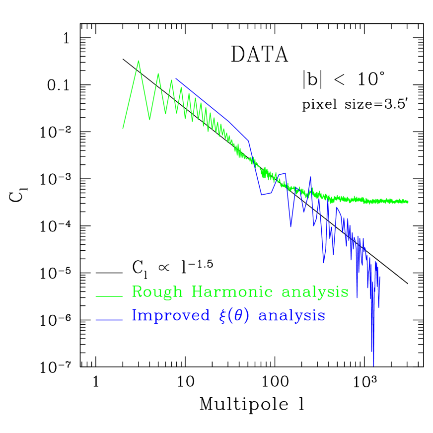
5.1.1 Rough Harmonic Analysis

We aim at computing the PS of the starlight polarization degree data according to Eq(9). In order to do so, we have generated a full-sky map (we use a HEALPix tessellation, see http://www.eso.org/kgorski/healpix) for stars at $|{\rm b}|<10^{\circ}$, which comprises 4114 stars, i.e, non-zero pixels (see Table 1). The resolution of the map has been chosen to be high enough ($3.5^{\prime}$ pixels) so that different sources are not identified with the same pixel. The PS of this map, shown in Fig(7) (see green line), has been computed using the anafast program of the HEALPix package. The slope of the PS is well-fitted by $C_{\ell}\propto\ell^{-1.5}$ down to $\ell\mathrel{\hbox to0.0pt{\lower 3.0pt\hbox{$\mathchar 536\relax$}\hss}\raise 2.0pt\hbox{$\mathchar 316\relax$}}100$ which translates into angular scales $\theta\mathrel{\hbox to0.0pt{\lower 3.0pt\hbox{$\mathchar 536\relax$}\hss}\raise 2.0pt\hbox{$\mathchar 318\relax$}}2^{\circ}$. On smaller scales $\theta\mathrel{\hbox to0.0pt{\lower 3.0pt\hbox{$\mathchar 536\relax$}\hss}\raise 2.0pt\hbox{$\mathchar 316\relax$}}2^{\circ}$, the PS is dominated by a flat shot-noise-like spectrum ($C_{\ell}=constant$), which is due to the effect of the large number of quasi-randomly located zero-valued pixels in the map, and which prevents us from measuring the PS of the underlying continuum signal down to the pixel resolution scale.

5.1.2 Improved Analysis: the Correlation Function Approach

In order to improve the simple analysis presented above, we should correct the data for the pixel window and the shot-noise intrinsic to the sparsely distributed data we want to analyze.

For this purpose we first compute the two-point correlation function of the polarization degree data using a quadratic estimator where the weighting is effectively done in pixel space
(Szapudi & Szalay 1998; see also Szapudi et al 2001). The method consists of the following steps:

• Compute the correlation function $\xi(\theta)$ of the data on a very fine grid of $\theta$ (typically 300000 bins).

• Resample the grid at the roots of the Legendre polynomial of order $\ell_{max}$, where $\ell_{max}$ is the maximum multipole at which one wishes to estimate the PS. The re-sampling, using a Gaussian interpolating kernel on the fine bins, weighted by the number of pairs per bin, is at the core of the method (see Szapudi et al 2001 for details).

• Obtain the PS by a simple Gauss-Legendre quadrature integration. The output is presented as flat band powers i.e, data averaged in multipole bins of width $\Delta\ell=20$.

The advantage of this method (with respect to the Harmonic approach) is that it gives an unbiased estimate of the power spectrum for an arbitrary sampling of the sky, thus avoiding the shot-noise power bias that is visible in the traditional PS estimator, as given by Eq(9). In turn this typically translates into a noisy estimate for the range of $\ell$’s where the shot-noise power dominates.

Fig 7 (see blue line) shows how this method allows for an efficient way of de-convolving the window function and removing the shot-noise component of the signal down to $\ell\approx 1000$, i.e, $\theta\approx 10^{\prime}$ which is close to the map resolution $\theta\approx 3.5^{\prime}$. Although the estimated signal is rather noisy on small scales $\ell\mathrel{\hbox to0.0pt{\lower 3.0pt\hbox{$\mathchar 536\relax$}\hss}\raise 2.0pt\hbox{$\mathchar 318\relax$}}100$, where the shot-noise dominates, the PS can be well-fitted on average by a power-law $C_{l}\propto\ell^{-1.5}$ in the whole range of scales measured, $\ell\mathrel{\hbox to0.0pt{\lower 3.0pt\hbox{$\mathchar 536\relax$}\hss}\raise 2.0pt\hbox{$\mathchar 316\relax$}}1000$.

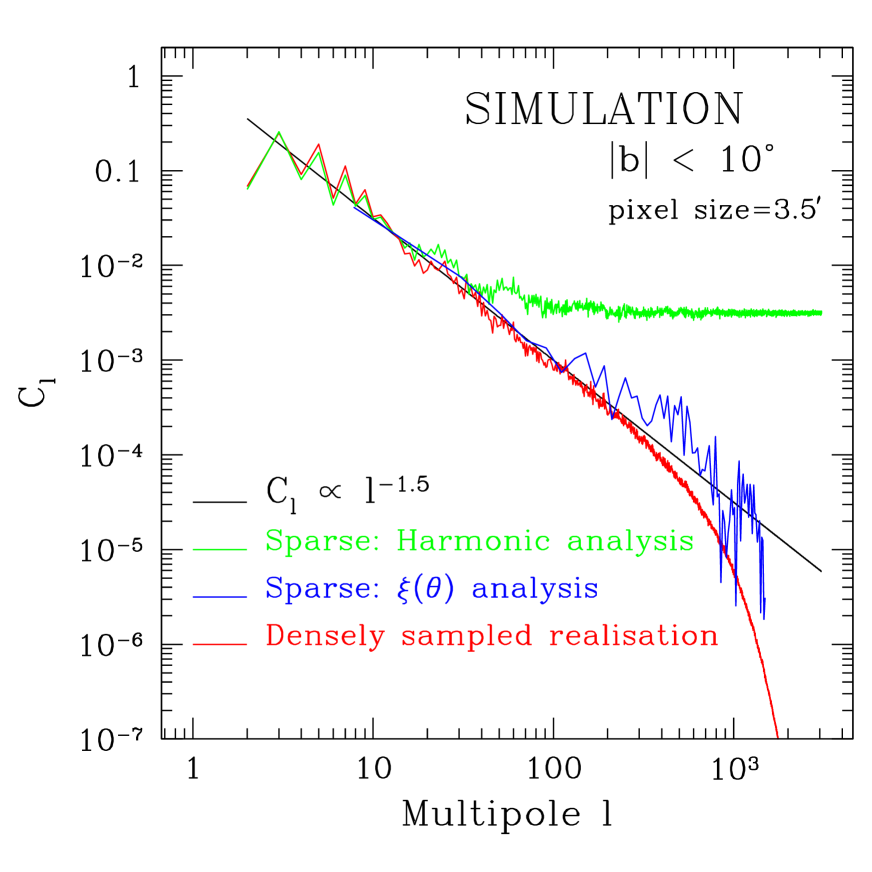
5.2 Power Spectrum Estimation of the Simulated Data

We would like to know how robust are the results obtained in the previous section. In particular, how sensitive is the estimated PS slope to the spatial distribution of stars used ? how does the clustering of the sources affect the PS analysis ? To answer these questions we have first simulated a mock starlight map in the Galactic plane ($|{\rm b}|<10^{\circ}$) for which we have computed the PS, as follows:

• Generate a random-Gaussian realization full-sky map of a $C_{\ell}\approx\ell^{-1.5}$ (with arbitrary amplitude), with the same spatial resolution than the original starlight data map ($3.5^{\prime}$ pixels). The latter PS gives a good fit to the starlight polarization degree PS for $\ell\mathrel{\hbox to0.0pt{\lower 3.0pt\hbox{$\mathchar 536\relax$}\hss}\raise 2.0pt\hbox{$\mathchar 316\relax$}}1000$, as shown in §5.1.

• Set all pixels outside the Galactic plane $|{\rm b}|<10^{\circ}$ to zero.

• Remove at random all but 4114 of the Galactic plane ($3.5^{\prime}$) pixels (or lines of sight) from the map. This leaves as many non-zero pixels from the random-Gaussian realization as in the original starlight data map (see Table 1).

• Compute the PS of the resulting sparsely sampled mock starlight map for the polarization degree as we did for the actual data according to the methods presented in §5.1.

As seen in Fig 8 (see green line), the rough harmonic analysis (see §5.1.1) shows that the simulated starlight data has approximately the same PS than the underlying densely sampled (effectively continuous) distributed data (red line) for multipoles $\ell\mathrel{\hbox to0.0pt{\lower 3.0pt\hbox{$\mathchar 536\relax$}\hss}\raise 2.0pt\hbox{$\mathchar 316\relax$}}40$ i.e, scales $\theta\mathrel{\hbox to0.0pt{\lower 3.0pt\hbox{$\mathchar 536\relax$}\hss}\raise 2.0pt\hbox{$\mathchar 318\relax$}}5^{\circ}$. On smaller scales, shot-noise dominates the signal. However, the improved analysis based on the correlation function approach (see §5.1.2) allows to measure the PS of the underlying continuous distributed map from the sparsely sampled mock starlight map down to much higher multipoles, $\ell\mathrel{\hbox to0.0pt{\lower 3.0pt\hbox{$\mathchar 536\relax$}\hss}\raise 2.0pt\hbox{$\mathchar 316\relax$}}1000$ i.e, scales $\theta\mathrel{\hbox to0.0pt{\lower 3.0pt\hbox{$\mathchar 536\relax$}\hss}\raise 2.0pt\hbox{$\mathchar 318\relax$}}10^{\prime}$ (see green line), although the signal is rather noisy beyond the shot-noise dominance scale $\ell\sim 40$.

5.3 Effect of Clustering

Since the mock starlight map was generated from a random-Gaussian realization, we can compare the PS analysis obtained from it (see §5.2) to the one performed on the real data (see §5.1), which are clearly non-Gaussian distributed (see Fig 9), to see what is the effect of clustering or non-Gaussianity in the distribution of the lines of sight.

Our findings in §5.2 show that the clustering of the sources in the analyzed starlight polarization degree map shifts the scale where shot-noise dominates from $\theta\approx 5^{\circ}$ down to $\theta\approx 2^{\circ}$. Therefore, a rough harmonic analysis allows a clean measurement of the PS of the underlying continuously distributed map down to much (a factor of 2.5) smaller scales when the sources are strongly clustered. However, using the improved correlation function analysis, shot-noise and pixel window effects can be effectively removed down to approximately the map resolution scale ($3.5^{\prime}$) with hardly any dependence on the clustering of the sources. The price to pay for this is that the more clustered the sources are, the noisier the measured PS turns out to be on small scales (see blue lines in Figs §7 & 8).

6 Discussion

In this paper we present an statistical analysis of the largest compilation available of Galactic starlight polarization data. The data analyzed consists of 5513 stars, a large fraction of which is found at low Galactic latitudes ($|{\rm b}|<10^{\circ}$) and in the vicinity of the sun (d $<$ 1 Kpc). Despite the inhomogeneous distribution of the sample, it allows for a proper statistical investigation of the large-scale behavior of the stellar parameters, such as the linear polarization (polarization degree and angle) and extinction, as induced by intervening dust grains.

The correlations between stellar parameters give some valuable information on the geometry and degree of uniformity of the Galactic magnetic field, as we discuss in §6.1 & §6.2. On the other hand, we discuss to what extent starlight data traces the the large-scale pattern of the polarized ISM in §6.3, based on our PS analysis (§5.1).

6.1 Polarization Angle and Magnetic Field Orientation

Although no consensus has been reached in relation to what mechanism is the dominant in the interstellar environment (see discussion in Lazarian 2000) it is generally accepted that grains in diffuse interstellar gas tend to be aligned with their major axes perpendicular to the magnetic field. The cases where the alignment is suspected to be parallel to magnetic field are extremely rare (see Rao et al 1998) and can be safely ignored in our analysis.

According to this picture, the electric field of radiation transmitted by an interstellar dust grain is less absorbed along the grain minor axis and therefore polarized in that direction which is parallel to the external magnetic field orientation. Therefore, polarized starlight radiation vectors are oriented parallel to the Galactic magnetic field.

Since starlight polarization vectors are only seen as projected in the plane of the sky, they just give us direct information on the plane-of-the-sky projection of the Galactic magnetic field orientation. In §4.2 we found a strong alignment of starlight polarization vectors with the Galactic plane structures and the spherical shell of Loop 1 (see §4.2 & §4.3), which in turn provides evidence that there is a net alignment of the magnetic field (as seen from its plane-of-the-sky projection) with Galactic structures on large-scales.

However, we stress that the full reconstruction of the 3D magnetic field orientations (and strength) requires additional complementary data from radio (synchrotron), sub-mm/IR (dust) observations and rotational measures from distant pulsars (Zweibel & Heiles 1997).

6.2 Polarization Degree and Efficiency of Magnetic Field Alignment

We have shown in our analysis that the starlight polarization degree and extinction are clearly correlated and on the mean, this correlation has a lower amplitude than what is expected from complete dust-grain alignment from homogeneous magnetic fields (see §4.1). The fact that starlight data exhibits a lower polarization degree as a function of extinction than the theoretical upper limit, suggests that either the grain alignment is not optimal or the Galactic magnetic field has a significant random component.

For grains in clouds with high extinction the alignment tends to fail (Lazarian et al 1997) but our sample does not deal with such clouds. At the same time, measurements of high degree of polarization suggest that the alignment can be sufficiently efficient. Substantial variations of the grain properties (e.g, the degree of elongation) do not look promising either.

On the other hand, a random component of the magnetic field ${\bf{B_{r}}}$ smears to some degree the correlation introduced by the uniform component ${\bf{B_{u}}}$ (Jones 1989). This smearing effect is likely to affect the observed stars as supported by the high degree of incoherence (randomness) observed for the starlight polarization angle (see Fig 11). In what follows we shall assume that the latter is the dominant misalignment effect to infer an upper limit in the degree of randomness of the Galactic magnetic field.

It is well-known that, by assuming a model, one can relate the observed polarization degree to the ratio of uniform to random plane-of-the-sky components of the underlying magnetic field (see e.g, Heiles 1996). In particular, assuming Burn’s model (Burn 1966), one finds for the starlight sample, Eq(4),

$${\rm{P_{Obs}\over P_{Max}}}={{\bf B^{2}_{u}}\over{{\bf B^{2}_{u}}+{\bf B^{2}_{r}}}}\approx 0.39-0.62$$ (11)

within the range, $0.1\mathrel{\hbox to0.0pt{\lower 3.0pt\hbox{$\mathchar 536\relax$}\hss}\raise 2.0pt\hbox{$\mathchar 316\relax$}}$ E(B-V) $\mathrel{\hbox to0.0pt{\lower 3.0pt\hbox{$\mathchar 536\relax$}\hss}\raise 2.0pt\hbox{$\mathchar 316\relax$}}1$, where the power-law is a good fit to ${P_{Obs}/P_{Max}}$ indeed. This yields, ${\bf{B_{u}}}/{\bf{B_{r}}}\approx 0.80-1.27$ for the same range. Note that Burn’s model assumes a 3D distribution of the random component (consistent with a scenario with a uniform field distorted by supernovae explosions) and a long enough path-length for every line of sight i.e, a large number of intervening clouds. In fact, for a subsample of nearby stars, the model tends to overestimate the ${\bf{B_{u}}}/{\bf{B_{r}}}$ ratio (Heiles 1996). Note that this bias is actually consistent with Eq(4) which predicts a larger ${\rm{P_{Obs}/P_{Max}}}$ for low extinction (or distance) and therefore, a larger ${\bf{B_{u}}}/{\bf{B_{r}}}$ ratio.

According to the above discussion, we take the value for high extinction E(B-V) $\mathrel{\hbox to0.0pt{\lower 3.0pt\hbox{$\mathchar 536\relax$}\hss}\raise 2.0pt\hbox{$\mathchar 318\relax$}}1$, which corresponds to distant stars (d $>$ 1 Kpc, see lower panel of Fig 3), as an unbiased estimate of the ratio, ${\bf{B_{u}}}/{\bf{B_{r}}}\approx 0.8$. This value is roughly consistent with previous estimates from starlight data (see Heiles 1996 for a review and references therein): ${\bf{B_{u}}}/{\bf{B_{r}}}\approx 0.68$. Note that ${\bf{B_{u}}}/{\bf{B_{r}}}$ as derived from starlight polarization data is typically larger than estimates from synchrotron polarization, ${\bf{B_{u}}}/{\bf{B_{r}}}\approx 0.54$, and it is significantly larger than that obtained from rotational measures of distant pulsars, ${\bf{B_{u}}}/{\bf{B_{r}}}\approx 0.28$.

The discrepancy between estimates from different data sets can be explained as every data set basically samples a different component of the interstellar medium: pulsars mainly trace the warm ionized medium, starlight data samples primarily the neutral media while synchrotron data seems to sample all components (Heiles 1996).

6.3 Large-scale Pattern of the Polarized ISM

We have performed an angular power spectrum (PS) analysis of the starlight polarization degree. We have focused on Galactic plane data ($|{\rm b}|<10^{\circ}$) as it concentrates most of the sources in the sample and therefore makes the statistical analysis more reliable. Our analysis shows that the starlight polarization degree PS is well fitted by a power-law behavior, $C_{\ell}\propto\ell^{-1.5}$ for $\ell\mathrel{\hbox to0.0pt{\lower 3.0pt\hbox{$\mathchar 536\relax$}\hss}\raise 2.0pt\hbox{$\mathchar 316\relax$}}1000$ (where the multipole order ${\ell}\approx 180^{\circ}/\theta$) which translates into angular scales ${\theta}\mathrel{\hbox to0.0pt{\lower 3.0pt\hbox{$\mathchar 536\relax$}\hss}\raise 2.0pt\hbox{$\mathchar 318\relax$}}10^{\prime}$. This is approximately the pixel resolution scale used, $3.5^{\prime}$ (see §5.1). This result was obtained thanks to a correlation function method which efficiently removes the shot-noise and pixel window effects that strongly affect the data on small scales (see §5.1.2).

We have assessed how the above results are affected by the clustering or non-Gaussianity in the distribution of sources by simulating a mock starlight map for the polarization degree (see §5.3). We found that the efficiency with which one measures the PS of the underlying densely-sampled signal is not significantly altered by the clustering of the sources, although for the real non-Gaussian distributed sources shot-noise dominates at smaller scales and the estimated PS is noisier than the simulated random-Gaussian case.

The above results provide evidence that the use of the polarization degree of the ISM as sparsely-sampled from lines-of-sight to several thousand (galactic-plane) stars allows a clean reconstruction of the PS of an underlying homogenelously sampled (continuum) polarization degree of the ISM. In particular, we find that the ISM polarization degree in the continumm has the same PS slope than that measured from sparsely-sampled data, $C_{\ell}\propto\ell^{-1.5}$.

The PS of the ISM dust polarization pattern happens to have a similar slope than that of the synchrotron Galactic polarization. Indeed, Baccigalupi et al (2001) showed that in the range of $1000>\ell>100$ the spectrum of polarised synchrotron continuum scales as $\ell^{1.7}$ with the uncertainty in the index $\pm 0.3$, which is compatible with the PS slope we find for the starlight polarization degree. However, synchrotron and aligned dust trace different phases of the ISM and the emission has, in principle, a completely different nature. Thus, on the first glance, one does not expect to see any correspondence between the two spectra. But if variations in the polarization arise mainly because of variations in the Galactic magnetic field, the properties of the two may be related. Further study shall show whether this similar statistical behaviour can be explained on physical grounds.

On the other hand, the lack of starlight data on high-galactic latitudes does not allow to make a reliable measurement of the PS for the moment. In particular, it remains to be seen whether the PS slope varies significantly at high-galactic latitudes in the same way as has been found in recent analyses from synchrotron emission (Baccigalupi et al 2000).

In a forthcoming paper (Fosalba et al 2001), we shall use our results on starlight data to model Galactic polarized dust emission at sub-mm/FIR wavelengths and its effect on the process of foreground subtraction in cosmic microwave background experiments.

Table 1: Mean Stellar Parameters: Sample of 5513 Stars

Latitude	Distance	Stars $(\%)$	P($\%$)	E(B-V)	$\theta_{p}$
	Total	$4114(75)$	$1.69$	$0.49$	$88.1$
Low Latitude	Nearby	$1451(26)$	$0.94$	$0.29$	$90.4$
	Distant	$2663(48)$	$2.09$	$0.60$	$86.9$
	Total	$1399(25)$	$0.45$	$0.15$	$93.0$
High Latitude	Nearby	$1315(24)$	$0.42$	$0.14$	$93.4$
	Distant	$84(1)$	$0.89$	$0.26$	$86.7$

Note. — Mean stellar parameters i.e, polarization degree P($\%$), extinction E(B-V), and polarization angle $\theta_{p}$, for the sample of 5513 stars analyzed, as a function of latitude and distance. High latitude (low latitude) means $|{\rm b}|>10^{\circ}$ ($|{\rm b}|<10^{\circ}$) and nearby (distant) denotes d $<$ 1 Kpc (d $>$ 1 Kpc).

Figure 1: Distribution of starlight polarization data in Galactic longitude and latitude bins (top panel) and distance and latitude bins (bottom panel) for the subsample of 5513 stars analyzed.

Figure 2: Distribution of sources with Galactic latitude, distance, polarization degree and extinction. In the top panel, the number of stars in the two central bins are displayed beside them as they are far above the plotted range.

Figure 3: Polarization degree with (quoted) error bars (top panel) and extinction (bottom panel) in linear distance bins. Solid lines show best fit curves to third order polynomials, Eqs(1) & (2).

Figure 4: Correlation between polarization degree P($\%$), and extinction E(B-V). Upper panel shows all individual sources while lower panel displays data averaged in extinction bins. Solid line shows the theoretical upper limit, P($\%$) = 9 E(B-V), for completely aligned grains by external (regular) magnetic fields. Dashed line in lower panel shows P($\%$) = 0.39 E(B-V)^0.8, which is a good fit to the data up to E(B-V) $\approx 1$.

Figure 5: Starlight Polarization Degree (top panel) and q parameter (bottom panel) for data averaged in 10^∘ longitude bins. The solid line shows a best fit to a sinusoidal dependence, Eqs(5) & (6).

Figure 6: Starlight Polarization Degree (top panel) and q parameter (bottom panel) for data averaged in 10^∘ latitude bins. The solid line in the upper panel shows a co-secant law distribution, Eq(7).

Figure 7: Angular power spectrum (PS) of the starlight polarization degree map in the Galactic plane, $|{\rm b}|<10^{\circ}$, which contains 4114 lines of sight. The PS estimation from the rough harmonic analysis (green line) is dominated by shot-noise for multipoles $\ell\mathrel{\hbox to0.0pt{\lower 3.0pt\hbox{$\mathchar 536\relax$}\hss}\raise 2.0pt\hbox{$\mathchar 318\relax$}}100$ i.e, angular scales $\theta\mathrel{\hbox to0.0pt{\lower 3.0pt\hbox{$\mathchar 536\relax$}\hss}\raise 2.0pt\hbox{$\mathchar 316\relax$}}2^{\circ}$. The improved correlation function analysis (blue line), which corrects for shot-noise and pixel window effects, shows that the underlying continuum signal can be well-fitted by $C_{\ell}\propto\ell^{-1.5}$ (black line) down to multipoles $\ell\approx 1000$ i.e, scales $\theta\approx 10^{\prime}$.

Figure 8: Same as Fig 7 but for the simulated starlight polarization degree map. The red line shows the densely-sampled (homogeneous) random-Gaussian realization of $C_{\ell}\propto\ell^{-1.5}$. The damping tail for $\ell\mathrel{\hbox to0.0pt{\lower 3.0pt\hbox{$\mathchar 536\relax$}\hss}\raise 2.0pt\hbox{$\mathchar 318\relax$}}200$ is due to the pixel window. The PS estimation from the rough harmonic analysis (green line) is dominated by shot-noise for multipoles $\ell\mathrel{\hbox to0.0pt{\lower 3.0pt\hbox{$\mathchar 536\relax$}\hss}\raise 2.0pt\hbox{$\mathchar 318\relax$}}40$ i.e, scales $\theta\mathrel{\hbox to0.0pt{\lower 3.0pt\hbox{$\mathchar 536\relax$}\hss}\raise 2.0pt\hbox{$\mathchar 316\relax$}}5^{\circ}$, while the improved correlation function analysis shows that the underlying continuum signal can be recovered down to multipoles $\ell\approx 1000$ i.e, up to scales $\theta\approx 10^{\prime}$.

Figure 9: Starlight Polarization Degree for the subsample of 5513 stars in Galactic coordinates. The map is shown in HEALPix tessellation with a pixel resolution of $1^{\circ}$ for convenience. Nearby stars (light-green sources) lie mainly at high Galactic latitudes while distant stars (red-purple sources) are found in the Galactic plane.

Figure 10: Same as Fig 9 but for Starlight Extinction, E(B-V). Sources with extinction E(B-V) $>2$ are not shown for clarity. A strong spatial correlation with the polarization degree distribution, Fig 9, is observed.

Figure 11: Same as Fig 9 but for the Starlight Polarization Angle. Note that, on large-scales, the polarization vectors are mostly aligned with the Galactic plane structure (light-green, light-blue and yellow sources) except for the spherical shell of Loop 1, where polarization vectors are roughly perpendicular to the Galactic plane (red sources).

References

- (1)
- Appenzaller (1974) Appenzeller I., 1974, A&A, 36, 99
- Baccigalupi et al (2000) Baccigalupi C., Burigana C., Perrotta F., De Zotti G., La Porta L., Maino D., Maris M., Paladini R., 2000, A&A, in Press [astro-ph/0009135]
- Bel et al (1993) Bel N., Lafon J.-P.J., Leroy J.L., 1993, A&A, 270, 444
- Berdyugin et al (1995) Berdyugin A., Snare M.-O., Teerikorpi P., 1995, A&A, 294, 568
- Burn (1966) Burn B.J., MNRAS, 1966, 133, 67
- de Oliveira-Costa & Tegmark (1999) de Oliveira-Costa A., Tegmark M., (eds) 1999, “Microwave Foregrounds”, ASP, V181
- Draine & Lazarian (1998) Draine B.T., Lazarian A.L., 1998, ApJ, 494, L19
- Draine & Lazarian (1999) Draine B.T., Lazarian A.L., 1999, in “Microwave Foregrounds” eds. A. de Oliveira-Costa and M. Tegmark, ASP, V181, 133
- Draine & Lee (1984) Draine B.T., Lee H.M., 1984, ApJ, 285, 89
- Draine & Weingartner (1996) Draine B.T., Weingartner J.C., 1996, ApJ, 470, 551
- Draine & Weingartner (1997) Draine B.T., Weingartner J.C., 1997 ApJ, 480, 633
- Fosalba et al (2001) Fosalba P., et al. 2001, in preparation
- Heiles (1996) Heiles C., 1996, ASP, in “Polarimetry of the Interstellar Medium” eds. W.G. Roberge and D.C.B. Whittet, V97, 457
-
Heiles (2000)
Heiles C., 2000, AJ, 119, 923
The data is publicly available by anonymous ftp at vermi.berkeley.edu. See pol15.out (compilation of data), and pol1.ps (description and references for the compiled data) in directory pub/polcat . It has also been recently made available through the web-sites:
http://vizier.u-strasbg.fr/viz-bin/VizieR?-source=II/226
http://adc.gsfc.nasa.gov/viz-bin/VizieR?-source=II/226
However, note that in these http addresses, no starlight extinction information is provided. - Heitsch et al (2001) Heitsch F., Zweibel E.G., Mac Low M-M., Li, P.S., Norman M.L., 2001, ApJ, in Press [astro-ph/0103286]
- Hildebrand et al (1995) Hildebrand R.H., Dotson J.L., Dowell C.D., Platt S.R., Schleuning D., Davidson J.A., Novak G., 1995, in “Airborne Astronomy Symposium on the Galactic Ecosystem: From Gas to Stars to Dust”, ASP, V73, 97
- Hildebrand & Dragovan (1995) Hildebrand R.H., Dragovan M., 1995, ApJ, 450, 663
- Hildebrand et al (1999) Hildebrand R.H., Dotson J.L., Dowell C.D., Schleuning D.A., Vaillancourt J.E., 1999, ApJ, 516, 834
- Hildebrand et al (2000) Hildebrand R.H., Davidson J.A., Dotson J.L., Dowell C.D., Novak G., Vaillancourt J. E., 2000, PASP, 112, 1215
- Jones (1989) Jones T.J., 1989, ApJ, 346, 728
- Kim & Martin (1995) S.-H., Kim, P.G., Martin, ApJ, 444, 293, 1995
- Korhonen & Reiz (1986) Korhonen T., Reiz A., 1986, A&A, 64, 487
- Krautter (1980) Krautter J., 1980, A&AS, 39, 167
- Lazarian et al (1997) Lazarian A., Goodman A., Myers P., 1997, ApJ, 490, 273
- Lazarian (2000) Lazarian A., 2000, in “Cosmic Evolution and Galaxy Formation”, ASP, eds. J. Franco, E. Terlevich, O. Lopez-Cruz, I. Aretxaga, V215, 69, [astro-ph/0003314]
- Lazarian (2001) Lazarian A., 2001, astro-ph/0101001
- Leroy (1993) Leroy J.L., 1993, A&A, 274, 203
- Markkanen (1979) Markkanen T., 1979, A&A, 74, 201
- Mathewson et al (1978) Mathewson D.S., Ford V.I., Klare G., Neckel T., Krautter J., 1978, Bull. Inf. CDS, 14, 115
- Novak et al (2000) Novak G., Dotson J.L., Dowell C.D., Hildebrand R.H., Renbarger T., Schleuning D.A., 2000, ApJ, 529, 241
- Prunet & Lazarian (1999) Prunet S., Lazarian A., 1999, in “Microwave Foregrounds” eds. A. de Oliveira-Costa and M. Tegmark, ASP, V181, 113
- Reiz & Franco (1998) Reiz A., Franco G.A.P., 1998, A&AS, 130, 133
- Rao et al (1998) Rao R., Crutcher R.M., Plambeck R.L., Wright M.C.H., 1998, ApJ, 502, L75
- Schroeder (1976) Schroeder R., 1976, A&AS, 23, 125
- Szapudi & Szalay (1998) Szapudi I., Szalay A.S., 1998, ApJ, 494, L41
- Szapudi et al (2001) Szapudi I., Prunet S., Pogosyan D., Szalay A.S. Bond J.R., 2001, ApJ, 548, L115
- Tucci et al (2000) Tucci M., Carretti E., Cecchini S., Fabri R., Orsini M., Pierpaoli E., 2000, NA, 5, 181
- Whittet (1992) Whittet D.C.B., 1992, “Dust in the Galactic Environment”, IOP Publishing, London.
- Zweibel & Heiles (1997) Zweibel E.G., Heiles C., 1997, Nature, 235, 131