On the Distribution of Haloes, Galaxies and Mass

Abstract

The stochasticity in the distribution of dark haloes in the cosmic density field is reflected in the distribution function $P_{V}(N_{h}|\delta_{m})$ which gives the probability of finding $N_{h}$ haloes in a volume $V$ with mass density contrast $\delta_{m}$. We study the properties of this function using high-resolution $N$-body simulations, and find that $P_{V}(N_{n}|\delta_{m})$ is significantly non-Poisson. The ratio between the variance and the mean goes from $\sim 1$ (Poisson) at $1+\delta_{m}\ll 1$ to $<1$ (sub-Poisson) at $1+\delta_{m}\sim 1$ to $>1$ (super-Poisson) at $1+\delta_{m}\gg 1$. The mean bias relation is found to be well described by halo bias models based on the Press-Schechter formalism. The sub-Poisson variance can be explained as a result of halo-exclusion while the super-Poisson variance at high $\delta_{m}$ may be explained as a result of halo clustering. A simple phenomenological model is proposed to describe the behavior of the variance as a function of $\delta_{m}$. Galaxy distribution in the cosmic density field predicted by semi-analytic models of galaxy formation shows similar stochastic behavior. We discuss the implications of the stochasticity in halo bias to the modelling of higher-order moments of dark haloes and of galaxies.

1 Introduction

In the current scenario of galaxy formation, galaxies are assumed to form by the cooling and condensation of gas within dark matter haloes (e.g. White & Rees 1978; White & Frenk 1991). The problem of galaxy clustering in space can therefore be approached by understanding the spatial distribution of dark haloes and the formation of galaxies in individual dark haloes. This approach to the problem of galaxy spatial clustering is very useful because the formation and clustering properties of dark haloes can be modelled relatively reliably due to the simplicity of the physics involved (gravity only) and because realistic models of galaxy formation in dark haloes can now be constructed using semi-analytic models (e.g. Kauffmann et al. 1999; Cole et al. 2000; Somerville & Primack 1999). Indeed, there are quite a few recent investigations attempting to model galaxy clustering based on the halo scenario (e.g. Jing et al. 1998; Ma & Fry 2000; Scoccimarro et al. 2001; Peacock & Smith 2000; Seljak 2000; Sheth et al. 2001).

Based on the Press-Schechter formalism (Press & Schechter 1974) and its extensions (Lacey & Cole 1994), Mo & White (1996) (hereafter MW) developed a model for the mean bias relation for dark haloes. Their model and its extension based on ellipsoidal collapse (Sheth et al. 2001) have been extensively tested by N-body simulations (e.g. MW; Mo et al. 1996; Jing et al. 1998; Sheth & Tormen 1999; Governato et al. 1999; Colberg et al. 2000). High-order moments of the halo distribution have also been modeled by Mo et al. (1997) based on a deterministic bias relation. These authors showed that the model works on large scales in comparison with N-body simulations. Nevertheless, the effect of stochasticity may be important in these high-order statistics as well as in the full distribution function of haloes. In fact, the non-Poissonian behavior of the bias relation is already emphasized in the original paper of MW; in particular, MW pointed out that halo-exclusion can cause sub-Poisson variance. Sheth & Lemson (1999) showed how the effects of stochasticity could be incorporated, easily and efficiently, into the analysis of the higher order moments.

Recently Somerville et al. (2001) used $N$-body simulations to study the stochasticity and non-linearity of the bias relation based on the formalism developed by Dekel & Lahav (1999). They analyzed the bias relation for haloes with masses larger than $1.0\times 10^{12}~{}h^{-1}~{}M_{\odot}$ in spherical volumes of radius $8\,h^{-1}{\rm{Mpc}}$. Our present work is quite closely related to theirs but contains several distinct aspects. First of all, our analysis is focused on the distribution function $P_{V}(N_{h}|\delta_{m})$, which gives the probability of finding $N_{h}$ haloes in a volume $V$ with mass density contrast $\delta_{m}$ [$\delta_{m}\equiv{\rho\over{\overline{\rho}}}-1$, where $\rho$ is the mass density and ${\overline{\rho}}$ is the mean mass density]. As we will show later, this function completely specifies the relation between the spatial distribution of haloes and that of the mass in a statistical sense. Second, our analysis covers a wider range of halo masses and a larger range of volumes for the counts-in-cells. Finally, we attempt to develop a theoretical model to describe the stochasticity of the bias relation. This theoretical model is based on the mean bias relation given in MW and on the variance model given in Sheth & Lemson (1999). As we will see below, the Sheth & Lemson model fails in high mass density regions, where gravitational clustering becomes important. One of the main purposes of this paper is to show that a simple modification of the Sheth & Lemson formulae for the variance allows one to make accurate predictions even in dense regions. Taruya & Suto (2000) have proposed a model for the stochasticity in halo bias relation based on the formation-epoch distribution of dark haloes, an approach very different from ours.

The paper is organized as follows. In Section 2 we introduce the bias relation based on the conditional probability and present a phenomenological model to describe the behavior of the variance as a function of the local density contrast. In Section 3 we present the numerical data used and study the mean and variance of the bias relation. We discuss and summarize our results in Section 4.

2 The Halo-Mass Bias Relation

2.1 The Concept of Bias

In the following we shall introduce some important concepts we will use throughout the paper. For simplicity we introduce them for the case of dark matter haloes, without loss of generality.

Let us define $\rho$ as the mass density smoothed in regions of some given volume $V$. The mass density contrast ($\delta_{m}$) in this volume is then defined as:

$$\delta_{m}\equiv{\rho\over{\overline{\rho}}}-1,$$ (1)

where ${\overline{\rho}}$ is the mean mass density in the universe. In the same way, if $N_{h}$ and $\overline{N}_{h}$ correspond to the number of dark matter haloes and to the mean number of dark matter haloes in the volume $V$, respectively, the number density contrast of dark matter haloes ($\delta_{h}$) is given by

$$\delta_{h}\equiv{N_{h}\over{\overline{N}_{h}}}-1.$$ (2)

The relationship between $\delta_{h}$ and $\delta_{m}$ is widely known as the halo-mass bias. A general way to represent this bias relation is to express the halo number density contrast as a function of the mass density contrast

$$\delta_{h}(V)\equiv F(\delta_{m}(V)).$$ (3)

Since the mass and halo number density contrasts are defined in a given volume, the bias relation defined in equation 3 is assumed to be a function of the local fields and thus called “local halo-mass bias”. The exact form of the function $F(\delta_{m}(V))$ depends on how the objects in consideration form in the cosmic density field.

The bias function $F(\delta_{m}(V))$ can be of several kinds. If the bias function is a linear function of the local mass density contrast $\delta_{m}(V)$ then it is said that one has linear bias. On the other hand, if the bias function is a non-linear function of the local mass density contrast $\delta_{m}(V)$ then one has non-linear bias. A special case occurs when $F(\delta_{m}(V))=\delta_{m}(V)$, in this case the local halo field is unbiased respect to the local mass density field.

The above mentioned biasing schemes correspond to the case of deterministic bias. A more general description of the biasing process corresponds to a stochastic one, i.e, there is a non-zero dispersion of the bias around its mean and the bias relation is described in a probabilistic way. There are two factors which can cause such dispersion. First, for a given region, not only $\delta_{m}$, but also other local properties, such as clumpiness and deviation from spherical symmetry, can affect the halo number in the region. Second, some non-local effects, such as the large-scale tidal field, can affect the formation of haloes. In general the stochasticity of the bias relation can be described by the conditional distribution function, $P_{V}(N_{h}|\delta_{m})$, which gives the probability of finding $N_{h}$ haloes in a volume $V$ with mass density contrast $\delta_{m}$. The deterministic bias scheme is recovered when the conditional probability can be well approximated by a delta function.

2.2 The conditional probability

Dark matter haloes are formed in the cosmological density field due to nonlinear gravitational collapse. In general, the halo density field is expected to be correlated with the underlying mass density field. Thus, if we denote by $\delta_{m}$ the matter density fluctuations field and by $N_{h}$ the field of halo number (where both fields are smoothed in regions of some given volume), $N_{h}$ and $\delta_{m}$ are related. We refer to this relation as the halo bias relation (see last subsection). Since in general the halo number in a volume depends not only on the mean mass density but also on other properties of the volume, the relation between $N_{h}$ and $\delta_{m}$ is not expected to be deterministic. It must be stochastic. The stochasticity of the bias relation can be described by the conditional distribution function, $P_{V}(N_{h}|\delta_{m})$, which gives the probability of finding $N_{h}$ haloes in a volume $V$ with mass density contrast $\delta_{m}$. This conditional probability completely specifies the relation between the mass and halo density fields in a statistical sense. Indeed, once $P_{V}(N_{h}|\delta_{m})$ is known, the full count-in-cell function $P_{V}(N_{h})$ for haloes can be obtained from the mass distribution function $P_{V}(\delta_{m})$ through

$$P_{V}(N_{h})=\int_{-\infty}^{\infty}{P_{V}(N_{h}\mid\delta_{m})P_{V}(\delta_{m})\,d\delta_{m}}.$$ (4)

The form of $P_{V}(N_{h}|\delta_{m})$ depends on how dark haloes form in the cosmological density field and is not known a priori. The simplest stochastic assumption is that it is Poissonian. This assumption is in fact used in almost all interpretations of the moments of galaxy counts in cells (c.f. Peebles 1980), where terms of Poisson shot noise are subtracted to obtain the correlation strength of the underlying density field. However, this assumption is not solidly based, and so it is important to examine if other assumptions on the form of $P_{V}(N_{h}|\delta_{m})$ actually work better for dark haloes. In this paper, we test other three models of $P_{V}(N_{h}|\delta_{m})$, along with the Poisson model. These are the Gaussian model, the Lognormal model, and the thermodynamical model. The last model was developed by Saslaw & Hamilton (1984) for the distribution of galaxies.

2.3 A Model for the Halo-Mass Bias Relation

To second order, the probability distribution function $P_{V}(N_{h}|\delta_{m})$ is described by the mean bias relation $N=N(\delta_{m})$ and the variance $\sigma^{2}\equiv\langle N^{2}|\delta_{m}\rangle$. MW developed a model for the mean bias relation of haloes based on the spherical collapse model. Their model works well for massive haloes and an extension of it by Sheth et al. (2001) based on ellipsoidal collapse may work better for low mass haloes.

Sheth & Lemson (1999) have presented a model for the variance of the bias relation which accounts for the halo exclusion due to the finite size of haloes (i.e. two different haloes can not occupy the same volume). They showed that their model was able to describe the first and second moments of the halo distribution from scale-free N-body simulations. Nevertheless the model is expected to fail when the underlying clustering makes a significant contribution to the variance. As an amendment, we introduce an additional term accounting for the clustering of haloes in high density regions. We use this phenomenological model for the variance of the halo bias relation.

Briefly, the mean of the bias relation from the MW model and our phenomenological modification of the Sheth & Lemson (1999) formula for the variance, are given by

$$\langle N\rangle=\int{dm~{}N(m,\delta_{1}\mid M,\delta_{0})}$$ (5)

and

$$\sigma^{2}=\langle N(N-1)\rangle+\langle N\rangle-\langle N\rangle^{2},$$ (6)

where:

$$\langle N(N-1)\rangle = \int{dm_{1}\,dm_{2}\ N(m_{1},\delta_{1}\mid M,\delta_{0})}$$ (7)

$$~{}~{}~{}N(m_{2},\delta_{1}\mid M-m_{1},\delta^{\prime})(1+A\overline{\xi}_{2}),$$

$N(m,\delta_{1}\mid M,\delta_{0})$ denotes the average number of haloes of mass $m$ identified at a given epoch $z_{1}$ [with a critical overdensity for collapse $\delta_{1}=\delta_{c}(1+z_{1})$] in an uncollapsed spherical region of comoving volume $V$ with mass $M$ and overdensity $\delta_{0}$, and $\delta^{\prime}$ is the mass density contrast of the fraction of the volume not occupied by the $m$ haloes. The additional term $(1+A\overline{\xi}_{2})$ in the expression for the variance accounts for the contribution from mass clustering and has been constructed as the simplest function of the variance of the mass distribution with the property of having high values in overdense regions and of being unity in homogeneous regions. As we will show below, a good fit to the simulation data can be achieved by choosing ${\overline{\xi}}_{2}$ to be the second order moment of the mass distribution on the scale in consideration. In this case, we can write the term $A{\overline{\xi}}_{2}=A{\overline{\xi}}_{m}(z_{1})\approx AD^{2}(z_{1}){\overline{\xi}}_{m}(0)$, where $D(z)$ is the linear growth factor normalized to one at $z=0$. The constant $A$ is to be calibrated by simulations.

3 Test by $N$-Body Simulations

3.1 Numerical Data

For this study we use the spatial distribution of dark matter particles as well as of dark haloes from the $\Lambda$CDM version of the high resolution GIF N-body simulations (for details see Kauffmann et al. 1999). These simulations have $256^{3}$ particles in a grid of $512^{3}$ cells, with a gravitational softening length of $20\,{h^{-1}{\rm kpc}}$. In the $\Lambda$CDM case, the simulation assumes $\Omega=0.3$, $\Omega_{\Lambda}=0.7$ and $h=0.7$. The initial power spectrum has a shape parameter $\Gamma=0.21$ and is normalized so that the rms of the linear mass density in a sphere of radius $8\,h^{-1}{\rm{Mpc}}$ is $\sigma_{8}=0.9$. The simulation box has a side length $L=141\,h^{-1}{\rm{Mpc}}$, and the mass of each particle is $M_{p}=1.4\times 10^{10}~{}h^{-1}{\rm M_{\odot}}$.

The halo catalogues have been created by the GIF project (Kauffmann et al. 1999) using a friends-of-friends group-finder algorithm to locate virialized clumps of dark matter particles in the simulations outputs. They used a linking length of 0.2 times the mean interparticle separation and the minimum allowed mass of a halo is 10 particles. In what follows, the mass of a halo is represented by the number of particles it contains.

We also use the galaxy catalogues constructed from the same simulations. The catalogues are limited to model galaxies with stellar masses greater than $\sim 2\times 10^{10}~{}h^{-1}M_{\odot}$. For further details about these catalogues and the galaxy formation models used in their construction see Kauffmann et al. (1999).

The halo conditional probability $P_{V}(N_{h}\mid\delta_{m})$ has been estimated for various samples and a number of sampling volumes $V$. For the presentation, we only use samples of haloes selected at redshifts $z=3$, 1 and 0. Two kinds of analyses are performed. In the first case, halo counts-in-cells are estimated at the same time as when the haloes are identified, while in the second case counts-in-cells are estimated at a given time for the central particles of the haloes identified at an earlier time. As a convention, we use $z_{1}$ to denote the redshift at which haloes are identified, while using $z_{0}$ to denote the redshift at which the counts in cells are estimated. For example, a case with $z_{0}=0$ and $z_{1}=3$ means that haloes are identified at redshift $3$ while the counts-in-cells are estimated for their central particles at redshift $0$. The computations of the counts in cells are performed for volumes of cubical cells with side lengths 1/32, 1/16, 1/8, and 1/4 times the side length of the simulation box, corresponding to $4.4$, 8.8, 17.6 and $35.2\,h^{-1}{\rm{Mpc}}$ in comoving units. The algorithm proposed by Szapudi et al. (1999), which allows an accurate determination of the probability function in a relatively short time, is applied to estimate the counts-in-cells on a grid of $256^{3}$ cells. The conditional probability of finding $N_{h}$ haloes in a cell of volume $V$ given that the local mean mass overdensity has a value between $\delta_{m}$ and $\delta_{m}+\Delta\delta_{m}$ is computed from the counts-in-cells through

$$P_{V}(N_{h}|\delta_{m})=\frac{P(N_{h},\delta_{m})\,\Delta\delta_{m}}{P(\delta_{m})\Delta\delta_{m}},$$ (8)

where $P_{V}(N_{h},\delta_{m})$ is the joint probability for finding $N_{h}$ haloes and a mass overdensity between $\delta_{m}$ and $\delta_{m}+\Delta\delta_{m}$ in a cell of volume $V$, and $P_{V}(\delta_{m})$ is the distribution function for the underlying mass density field.

3.2 The Conditional Probability

Figure 1 shows the conditional probability $P_{V}(N_{h}|\delta_{m})$ obtained from the simulations at several representative values of $\delta_{m}$. The halo sample shown contains all present-day haloes with masses greater than 10 particles. The numerical conditional probabilities are compared with the fits to Gaussian, Lognormal, Poisson and Thermodynamical functions. From the figure it can bee seen that the Poisson model is in general a poor description of the present time conditional probability measured from the simulations, and that the Gaussian model is overall a quite good assumption. The Lognormal and Thermodynamical functions are a sort of intermediate functions, i.e they are not as poor descriptors for the conditional probability as the Poisson function is, but, on the other hand, they do not describe the features of the conditional function as good as the Gaussian function does. This result is valid for all the halo mass ranges under analysis and all the scales tested.

As discussed by Coles & Frenk (1991), the widely used Poisson model introduced by Layzer (1956) is based on the assumption that the probability to find a given number of galaxies (or haloes) in a volume is determined only by the local mass density field and that the probability to find a galaxy (or halo) in an infinitesimal volume $\delta V$ is proportional to the density at this volume element and is independent of the probability to find another galaxy (or halo) in a neighboring infinitesimal volume. Therefore, our finding that the conditional probability for haloes has non-Poisson form suggests that the deviation from Poisson of the halo-biasing process is due to effects related to the probability for a halo to have neighbors, such as volume exclusion, clustering and large-scale environments. Notice that some of these effects are already included in the model for the variance of the bias relation (section 2.3).

Figure 1: Comparison between the conditional probability measured from the simulations (squares) for present epoch haloes with masses greater than 10 particles and the corresponding best fits of the Poisson (dash-dot-dot-dot line), Thermodynamical (dashed line), Lognormal (dash-dot line) and Gaussian (solid line) distribution functions. The rows correspond, from top to bottom, to the sampling scales $\ell=4.4,~{}8.8,~{}17.6,~{}35.2~{}Mpc/h$, respectively. For each sampling scale there are four plots corresponding to the local mass overdensity as indicated in the labels.

3.3 The Mean and Variance of Halo Bias

Given that the Gaussian model is a reasonable fit to the conditional probability function, we now concentrate on the mean and variance of this function, which are the two quantities needed to specify a Gaussian distribution. In order to show deviations from the Poisson distribution, we consider the mean and the ratio between the variance and the mean:

$$1+\delta_{h}\equiv{\langle N|\delta_{m}\rangle\over{\overline{n}}V},~{}~{}~{}~{}~{}~{}~{}{{\rm variance}\over{\rm mean}}\equiv{\sigma^{2}\over\langle N|\delta_{m}\rangle},$$ (9)

where $\delta_{h}\equiv{{N_{h}}\over{{\overline{n}}V}}-1$ is the number density contrast of haloes and ${\overline{n}}$ is their mean number density.

Figures 2-4 show the results given by the simulations. Results are shown for samples in four representative mass ranges: a) a sample of low mass haloes, b) a sample containing both low and high mass haloes, c) a sample of intermediate mass haloes and d) a sample of high mass haloes. The corresponding halo masses are shown in table 1.

Sample	$z_{1}=0$	$z_{1}=1$	$z_{1}=3$
a)	$M_{h}=20$–30 particles	$M_{h}=20$–30 particles	$M_{h}=20$–30 particles
	$M_{h}/M_{\star}=0.03$–0.04	$M_{h}/M_{\star}=0.62$–0.92	$M_{h}/M_{\star}=100$–150
b)	$M_{h}=20$–2000 particles	$M_{h}=20$–2000 particles	$M_{h}=20$–600 particles
	$M_{h}/M_{\star}=0.03$–2.85	$M_{h}/M_{\star}=0.62$–61.5	$M_{h}/M_{\star}=100$–3000
c)	$M_{h}=200$–800 particles	$M_{h}=200$–800 particles	$M_{h}=50$–100
	$M_{h}/M_{\star}=0.28$–1.14	$M_{h}/M_{\star}=6.15$–24.6	$M_{h}/M_{\star}=250$–500
d)	$M_{h}>800$ particles	$M_{h}>800$ particles	$M_{h}>200$
	$M_{h}/M_{\star}>1.14$	$M_{h}/M_{\star}>24.6$	$M_{h}/M_{\star}>1000$

Table 1: Ranges of halo masses corresponding to the samples shown in figures 2-4. a) sample of low mass haloes, b) sample containing both low and high mass haloes, c) sample of intermediate mass haloes and d) sample of high mass haloes. $M_{\star}$ is defined by $\sigma(M_{\star})=1.68$.

One sees that the ratio variance/mean shows a Poisson-like behavior (i.e. $\sim 1$) for low values of $\delta_{m}$. This ratio becomes sub-Poisson (i.e. $<1$) at intermediate values of $\delta_{m}$, and super-Poisson ($>1$) for high values of $\delta_{m}$. The exact change of the variance/mean ratio with $\delta_{m}$ depends on halo mass: the sub-Poisson variance extends to higher values of $\delta_{m}$ for samples with higher halo masses. The volume-exclusion effect is reduced for the descendants of haloes identified at an earlier epoch and the variance/mean ratio approaches the Poisson value for the descendants of haloes selected at early times (see Figure 4).

The curves in Figures 2-4 show model predictions. The mean bias relations given by the simulations are well described by the model of MW, confirming earlier results. The behavior of the variance/mean ratio is also reasonably well reproduced, when the constant $A$ in equation (6) is chosen to be 0.05 (as given by the fit to the bias relation for present-day haloes in the simulation). Thus, sub-Poisson variance can be caused by halo exclusion while the super-Poisson variance at high $\delta_{m}$ may be explained by the clustering of mass at the time of halo identification. The model for the variance begins to fail at very high values of $\delta_{m}$. But since cells with such high densities are only a tiny fraction of all cells, this failure is not important.

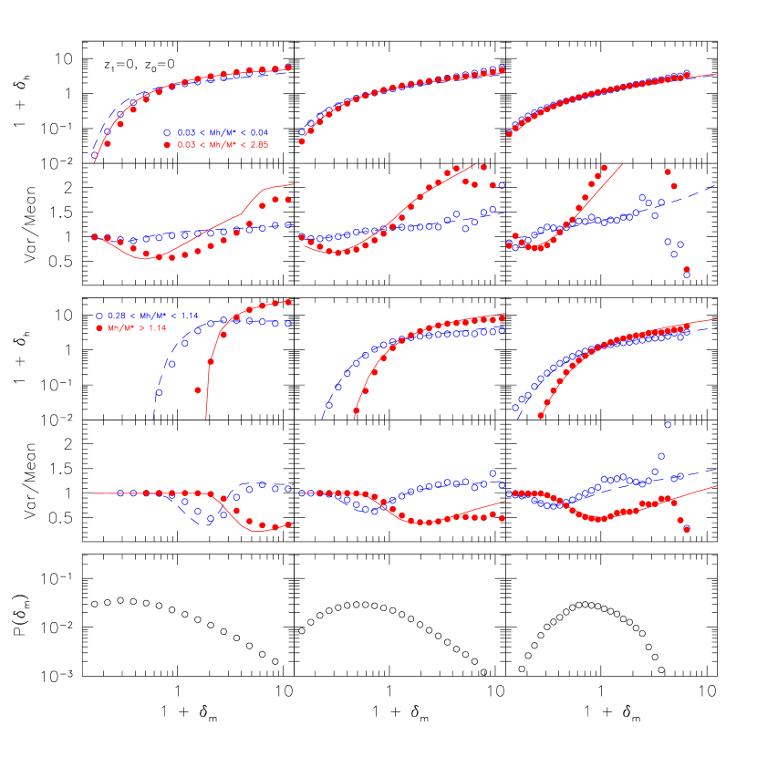
Figure 2: Theoretical predictions from the MW model for the mean and from our proposed phenomenological modification of the (Sheth & Lemson 1999) model for the variance of the bias relation (lines) compared with the corresponding quantities obtained from the GIF $\Lambda$CDM simulations (symbols). The columns correspond, from left to right, to the cell sizes $l=4.4$, $8.8$ and $17.6~{}Mpc/h$. The two upper panels show the mean of the bias relation (upper row in panel) and the ratio between the variance and the mean of the bias relation (lower row in panel) for the ranges of halo masses indicated in the respective labels. The dashed and solid lines show the theoretical predictions corresponding to the numerical data represented by the open and filled circles, respectively. The mass probability function at the respective scales is shown in the lowest panel. The sample corresponds to haloes identified and analyzed at the present epoch.

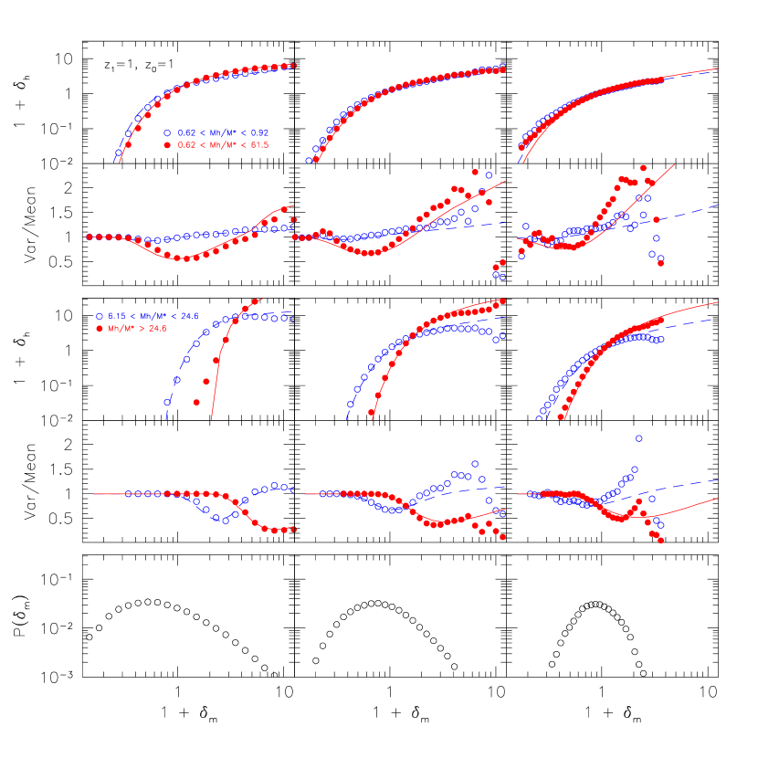
Figure 3: Same results as shown in figure (2) but for haloes identified and analyzed at redshift $z=1$.

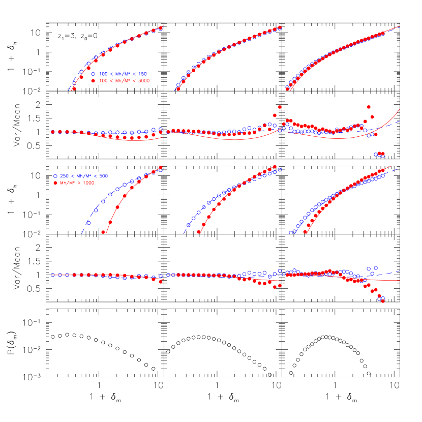
Figure 4: The same as in figure (2) but for the present epoch descendants of haloes already formed at $z=3$.

3.4 Bias Relation for Model Galaxies

We have also estimated the mean and variance of the bias relation between model galaxies, from the GIF simulations, with stellar masses greater than $\sim 2\times 10^{10}h^{-1}M_{\odot}$ and the underlying mass density, with the results shown in Figure 5. Interestingly, the variance/mean ratio in the galaxy-mass bias relation also exhibits significant sub-Poissonian behavior, implying that the effect of volume exclusion is also important for the spatial distribution of galaxies. One possible reason for this is that many of the galaxy-sized haloes may host only one galaxy and the galaxy distribution inherits a considerable fraction of the exclusion effects from the distribution of their host haloes.

If this is true for real galaxies, it has important implications for the interpretations of galaxy clustering, as we will see in Section 4.

3.5 The Count-in-Cell Function of Dark Haloes

As an additional test for the bias model, we use the simulation result for $P_{V}(\delta_{m})$ and the theoretical model for $P_{V}(N_{h}|\delta_{m})$ [i.e. a Gaussian conditional probability function with the mean and variance given by equations (2)-(4)] to reconstruct the counts-in-cells functions for haloes by using equation (4). As we only want to test the model of the bias relation, we do not use theoretical models for $P_{V}(\delta_{m})$, although such models do exist [e.g. the model of Sheth (1998) based on excursion set approach, and the Lognormal model used in Coles & Jones (1991)]. Since the probability functions obtained from the simulations are quite noisy at very high values of $\delta_{m}$ and the model predictions in this regime may fail, we truncate our computations at a given high value of $\delta_{m}$ [$\delta_{m}^{max}=10$ at the scales $l=4.4\ {\rm and}\ l=8.8~{}h^{-1}~{}Mpc$, and $\delta_{m}^{max}=3$ at $l=17.6~{}h^{-1}~{}Mpc$], which correspond to the low-probability tail of the mass probability function, as can be seen clearly in the lower panel in figure (2). For comparison we also reconstruct the halo count-in-cell functions using a Poissonian form for the conditional function, with the mean given by equation (2). In Figure (6) we compare the reconstructed halo count-in-cell functions for present-day haloes containing more than 10 particles with the corresponding functions obtained directly from the simulations. Clearly, the model matches the simulation results remarkably well. The halo count-in-cell functions reconstructed using a Poissonian form for the conditional probability function depart from the corresponding numerical values in the low-probability, high density tail.

The halo count-in-cell functions obtained through this approach can be used to calculate the high-order moments, such as skewness and kurtosis, of halo distributions. This application will be presented in detail in a forthcoming paper.

4 Discussion and Summary

In this paper, we have analyzed in detail the conditional probability function $P_{V}(N|\delta_{m})$ to understand the stochastic nature of halo bias. We have found that in high-resolution $N$-body simulations this function is well represented by a Gaussian model, and that a Poisson model is generally a poor approximation. That means that the galaxy biasing process, as well as the halo biasing process, is not only determined by the local value of the mass density field, but also by other local quantities, such as clumpiness, and by non-local properties, such as large-scale tidal field.

We have shown that a simple, phenomenological model can be constructed for $P_{V}(N|\delta_{m})$. This allows one to construct a theoretical model for the full count-in-cell function for dark haloes. The galaxy distribution in the cosmic density field predicted by semi-analytic models of galaxy formation shows similar stochastic behavior to that of the haloes, implying that galaxy distribution is not a Poisson sampling of the underlying density field.

These results have important implications in the interpretations of galaxy clustering in terms of the underlying density field. For example, the quantity conventionally used to characterize the second moment of counts-in-cells is defined (here for dark halo) as

$$\kappa_{2}(R)={\langle(N-{\overline{n}}V)^{2}\rangle\over({\overline{n}}V)^{2}}-{1\over({\overline{n}}V)},$$ (10)

where the second term on the right-hand side is to subtract Poisson shot noise (e.g. Peebles 1980). With the use of equation (4), it is easy to show that

$$\kappa_{2}(R) = {1\over({\overline{n}}V)^{2}}\int\langle N|\delta_{m}\rangle^{2}P_{V}(\delta_{m})\,d\delta_{m}$$ (11)

$$+ {1\over({\overline{n}}V)^{2}}\int\left[\sigma^{2}-\langle N|\delta_{m}\rangle\right]P_{V}(\delta_{m})\,d\delta_{m}-1\,.$$

Thus, even if haloes trace mass on average, i.e. $\langle N|\delta_{m}\rangle\propto\delta_{m}$, this quantity is not equal to the second moment for the mass, because the second term on the right-hand side is generally non-zero. Furthermore, the non-Poissonian behavior of the bias relation might imply that the (Poisson) shot-noise corrections usually applied at estimating higher-order moments of the galaxy distribution are not completely correct and therefore interpretations of skewness and kurtosis might change considerably, at least at the scales where shot-noise terms are not too small. This issue needs to be investigated in more detail. Thus, in order to infer the properties of the mass distribution in the Universe from statistical measures of the galaxy distribution, it is necessary to understand the stochastic nature of galaxy biasing.

As discussed in Dekel & Lahav (1999), the stochasticity in galaxy biasing not only affects the interpretation of the moments of the galaxy distribution, but also affects the interpretation of other statistical measures of galaxy clustering, such as redshift distortions, the cosmic virial theorem and the cosmic energy equation. With the results shown in the present paper, one can model quantitatively many of these effects.

Figure 5: Mean bias relation and ratio between the variance and the mean of the bias relation of galaxies obtained from the simulations using semi-analytical models of galaxy formation. We show model galaxies at the present epoch (upper panel) and at redshift $1$ (lower panel). The mean and ratio between the variance and the mean of the bias relation are shown in the top and bottom rows in each panel, respectively. At each epoch the cubical cells of side length, from left to right, $l=4.4,~{}8.8,~{}17.6~{}h^{-1}~{}Mpc$ are shown.

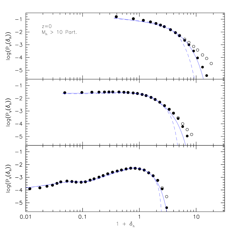
Figure 6: Halo count-in-cell functions for a sample of present day haloes with masses greater than 10 particles. The circles correspond to the probability function obtained from the simulations and the lines to the semi-analytically reconstructed count-in-cell function using spherical collapse approach. The solid and dashed lines show the reconstructed functions using a Gaussian and a Poissonian form for the conditional probability function, respectively. The open circles show the simulated halo count-in-cell functions obtained from the complete mass and conditional probability functions, while the filled circles show the simulated mass count-in-cell functions obtained from the mass and conditional probability functions truncated at high values of the mass density contrast. The boxes correspond, from top to bottom, to the scales $l=4.4,~{}8.8,~{}17.6~{}h^{-1}~{}Mpc$.

References

- Colberg et al. (2000) Colberg J. M., White S. D. M., Yoshida N., MacFarland T. J., Jenkins A., Frenk C. S., Pearce F. R., Evrard A. E., Couchman H. M. P., Efstathiou G., Peacock J. A., Thomas P. A., The Virgo Consortium 2000, MNRAS, 319, 209
- Cole et al. (2000) Cole S., Lacey C. G., Baugh C. M., Frenk C. S., 2000, MNRAS, 319, 168
- Coles & Frenk (1991) Coles P., Frenk C. S., 1991, MNRAS, 253, 727
- Coles & Jones (1991) Coles P., Jones B., 1991, MNRAS, 248, 1
- Dekel & Lahav (1999) Dekel A., Lahav O., 1999, ApJ, 520, 24
- Governato et al. (1999) Governato F., Babul A., Quinn T., Tozzi P., Baugh C. M., Katz N., Lake G., 1999, MNRAS, 307, 949
- Jing et al. (1998) Jing Y. P., Mo H. J., Boerner G., 1998, ApJ, 494, 1
- Kauffmann et al. (1999) Kauffmann G., Colberg J. M., Diaferio A., White S. D. M., 1999, MNRAS, 303, 188
- Lacey & Cole (1994) Lacey C., Cole S., 1994, MNRAS, 271, 676
- Layzer (1956) Layzer D., 1956, AJ, 61, 383+
- Ma & Fry (2000) Ma C. P., Fry J. N., 2000, ApJ, 531, 87
- Mo et al. (1997) Mo H., Jing Y. P., White S. D. M., 1997, MNRAS, 284, 189
- Mo et al. (1996) Mo H. J., Jing Y. P., White S. D. M., 1996, MNRAS, 282, 1096
- Mo & White (1996) Mo H. J., White S. D. M., 1996, MNRAS, 282, 347
- Peacock & Smith (2000) Peacock J. A., Smith R. E., 2000, MNRAS, 318, 1144
- Peebles (1980) Peebles P. J. E., 1980, The Large-Scale Structure of the Universe. Princeton Univ. Press
- Press & Schechter (1974) Press W. H., Schechter P., 1974, ApJ, 187, 425
- Saslaw & Hamilton (1984) Saslaw W. C., Hamilton A., 1984, ApJ, 276, 13
- Scoccimarro et al. (2001) Scoccimarro R., Sheth R. K., Hui L., Jain B., 2001, ApJ, 546, 20
- Seljak (2000) Seljak U., 2000, MNRAS, 318, 203
- Sheth (1998) Sheth R. K., 1998, MNRAS, 300, 1057
- Sheth & Lemson (1999) Sheth R. K., Lemson G., 1999, MNRAS, 304, 767
- Sheth et al. (2001) Sheth R. K., Mo H. J., Tormen G., 2001, MNRAS, 323, 1+
- Sheth & Tormen (1999) Sheth R. K., Tormen G., 1999, MNRAS, 308, 119
- Somerville et al. (2001) Somerville R. S., Lemson G., Sigad Y., Dekel A., Kauffmann G., White S. D. M., 2001, MNRAS, 320, 289
- Somerville & Primack (1999) Somerville R. S., Primack J. R., 1999, MNRAS, 310, 1087
- Szapudi et al. (1999) Szapudi I. ., Quinn T., Stadel J., Lake G., 1999, ApJ, 517, 54
- Taruya & Suto (2000) Taruya A., Suto Y., 2000, ApJ, 542, 559
- White & Frenk (1991) White S. D. M., Frenk C., 1991, ApJ, 379, 52
- White & Rees (1978) White S. D. M., Rees M. J., 1978, MNRAS, 183, 341