The Distance to SN 1999em from the Expanding Photosphere Method

Abstract

We present optical and infrared spectroscopy of the first two months of evolution of the Type II SN 1999em. We combine these data with high-quality optical/infrared photometry beginning only three days after shock breakout, in order to study the performance of the “Expanding Photosphere Method” (EPM) in the determination of distances. With this purpose we develop a technique to measure accurate photospheric velocities by cross-correlating observed and model spectra. The application of this technique to SN 1999em shows that we can reach an average uncertainty of 11% in velocity from an individual spectrum. Our analysis shows that EPM is quite robust to the effects of dust. In particular, the distances derived from the $VI$ filters change by only 7% when the adopted visual extinction in the host galaxy is varied by 0.45 mag. The superb time sampling of the $BVIZJHK$ light-curves of SN 1999em permits us to study the internal consistency of EPM and test the dilution factors computed from atmosphere models for Type II plateau supernovae. We find that, in the first week since explosion, the EPM distances are up to 50% lower than the average, possibly due the presence of circumstellar material. Over the following 65 days, on the other hand, our tests lend strong credence to the atmosphere models, and confirm previous claims that EPM can produce consistent distances without having to craft specific models to each supernova. This is particularly true for the $VI$ filters which yield distances with an internal consistency of 4%. From the whole set of $BVIZJHK$ photometry, we obtain an average distance of 7.5$\pm$0.5 Mpc, where the quoted uncertainty (7%) is a conservative estimate of the internal precision of the method obtained from the analysis of the first 70 days of the supernova evolution.

1 INTRODUCTION

The last ten years have witnessed an enormous progress in our knowledge of the optical properties of supernovae (SNe) of all types. However, comparatively little is still known about these objects in infrared (IR) wavelengths. Light-curves in the $JHK$ bands have been obtained only for a handful events since the pioneering work of Elias et al. (1981, 1985) on Type Ia SNe. Aside from SN 1987A (e.g. Suntzeff & Bouchet 1990), SN 1990E (Schmidt et al. 1993), and SN 1980K (Dwek et al. 1983), virtually nothing is known of the $JHK$ light curves of Type II SNe. The spectroscopic studies have been mostly limited to optical wavelengths (3000-10000 Å) also, and few spectra have been obtained beyond this range Bowers et al. (1997).

Given the rapid technological development of IR light detection over recent years, the next logical step is to expand the SN observations to the broadest possible spectral range. With this idea in mind, in 1999 we started a program to obtain optical and IR photometry and spectroscopy of nearby SNe ($z$$<$0.08), in order to better understanding 1) the nature of SNe, 2) the explosion mechanisms, 3) the relation of SN properties to their stellar environments, and 4) the use of SNe as distance indicators. The “Supernova Optical and Infrared Survey” (SOIRS) uses telescopes at Cerro Tololo Inter-American Observatory (CTIO), the Carnegie Institution of Washington at Las Campanas Observatory (LCO), the European Southern Observatory (ESO) at La Silla and Cerro Paranal, the Steward Observatory (SO) of The University of Arizona, and the Cerro El Roble observatory of the University of Chile. To ensure sufficient targets for the observing runs, we schedule SN search runs with the Maksutov camera at Cerro El Roble Maza et al. (1981), prior to the follow-up runs. With photographic film this camera permits us to sample a wide field of view (5^∘ x 5^∘) down to a limiting magnitude of 18. With this setup the photographic survey finds SNe up to $z$=0.08, which are ideally suited for the follow-up program. We also coordinate the follow-up runs with the Nearby Galaxies Supernova Survey (NGSS) carried out with the Kitt Peak 0.9-m telescope and the wide field mosaic CCD array, which discovers SNe down to a limiting magnitude of $R\sim$21 ($z$$<$0.15) Strolger et al. (1999). We include in our list of targets SNe found at other observatories and reported to the IAU Circulars.

In the course of 1999-2000 the SOIRS program has gathered high-quality observations for $\sim$20 SNe. In this paper we report observations of one of the best-observed objects included in our program, the Type II SN 1999em discovered on 1999 October 29 (JD 2451480.94) in the course of the Lick Observatory Supernova Search (Li, 1999). The supernova occurred in NGC 1637, a spiral galaxy with a heliocentric radial velocity of 717 km s^-1 Haynes et al. (1998). A pre-discovery image of NGC 1637 taken on October 20.45 showed nothing at the position of SN 1999em (with a limiting magnitude of $\sim$19.0), which indicated that the SN had been caught at an early stage. An optical spectrum taken one day later (October 30.34) showed that SN 1999em had the H line P-Cygni profiles characteristic of a Type II event. The blue continuum and the presence of the He I $\lambda$5876 line confirmed that SN 1999em had been found at an early epoch (Jha et al., 1999). Given its proximity and early evolutionary stage, SN 1999em proved to be an excellent target to test the “Expanding Photosphere Method” (EPM, hereafter) in detail, and determine the distance to the host galaxy.

The discovery of SN 1999em occurred right in the middle of a SOIRS observing campaign previously scheduled for 1999 October-December. As soon as the discovery of SN 1999em was reported, we decided to initiate a follow-up program in order to obtain high-quality data for this event. During this observing run we obtained superb optical and IR sampling of the first 180 days of the $UBVRIZJHK$ light-curves, as well as optical/IR spectroscopy for the first 60 days of the evolution of SN 1999em. Except for the sub-luminous/peculiar SN 1987A, this object is the best observed event of the Type II class to date.

All of the photometry for SN 1999em, except for the $Z$-band, was reduced and analyzed by Suntzeff et al. and will be published separately. In Sec. 2.1 we give a brief summary of these observations and describe the main features of the light-curves. Also, we report the $Z$-band photometry of SN 1999em. In Sec. 2.2 we summarize our spectroscopic observations and present the resulting spectra. In Sec. 3 we use the “Expanding Photosphere Method” (EPM) to compute the distance to the host galaxy, after which (Sec. 4) we discuss our results. Finally (Sec. 5), we present the main conclusions of this study. In Appendix A we summarize the basic ideas behind EPM and our implementation to compute distances to SNe II. Appendix B describes the details of computing the synthetic magnitudes required by EPM. Having defined our synthetic photometric system, in Appendix C we proceed to compute the distance correction factors from the SN II atmosphere models published by Eastman, Schmidt, & Kirshner (1996, E96 hereafter). In Appendix D we define the $Z$ photometric system and we list magnitudes for the standards that we used in our observations.

2 OBSERVATIONS AND REDUCTIONS

2.1 Photometry

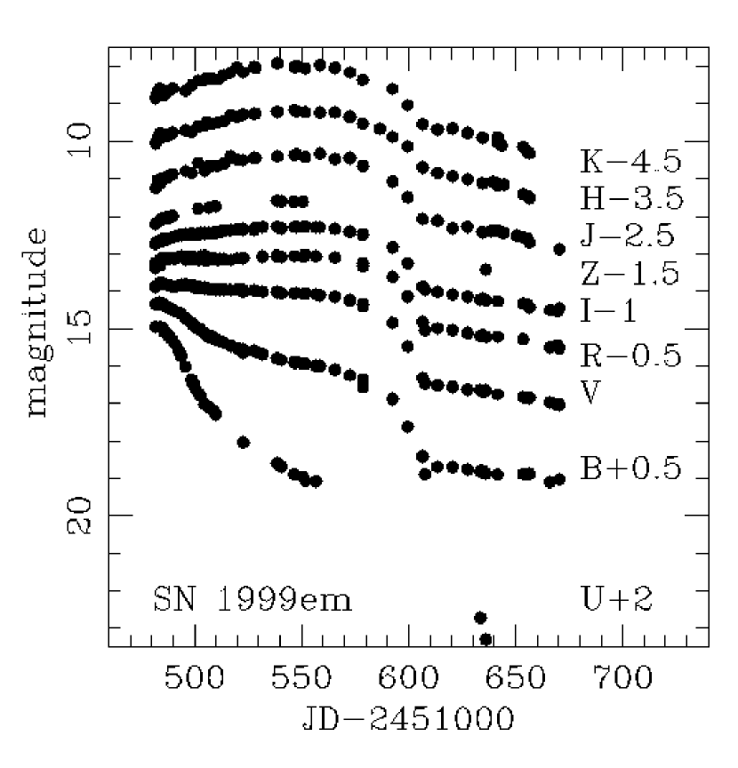
Figure 1: $UBVRIZJHK$ light-curves of SN 1999em.

We obtained extensive optical and IR photometric follow-up of SN 1999em covering 180 days from discovery until the SN went behind the Sun. The data will be presented in a separate paper by Suntzeff et al. (2001). Table 1 lists additional $UBVRI$ observations taken with the CTIO 1.5-m, SO 1.5-m, SO 2.3-m, and ESO NTT telescopes. We include in this table $Z$-band photometry gathered with the CTIO 0.9-m and reduced relative to a photometric sequence properly calibrated with respect to the standards listed in Appendix D. In what follows we adopt a minimum photometric error of 0.015 mag in order to account for photometric uncertainties beyond the photon statistics quoted by Suntzeff et al. Figure 1 presents the light-curves which reveal the exceptional sampling obtained. The $U$ light-curve shows that maximum light occurred just after discovery, on JD 2451482.8 (October 31), followed by a phase of rapid decline during which the SN dimmed by $\sim$4 mag in 70 days. The faintness of the SN made further observations through the $U$ filter difficult. The $B$ light-curve shows that maximum occurred two days later than in $U$, a rapid decline for $\sim$30 days during which the SN dimmed by $\sim$1 mag, a phase of 70 days of slowly-decreasing luminosity (plateau) during which the flux decreased by one additional magnitude, a fast drop in flux by 2.5 mag in only 30 days, and a linear decay in magnitude as of JD 2451610 that signaled the onset of the nebular phase. The $V$ light-curve was characterized by a plateau of nearly-constant brightness that lasted $\sim$100 days (until JD 2451590), followed by a drop of 2 mag in $\sim$30 days, and a linear decline at the slow pace of $\sim$0.01 mag day^-1. The $R$, $I$, $Z$, $J$, $H$, and $K$ light-curves had the same basic features of the $V$ light-curve, except that the SN gradually increased its luminosity during the plateau. The brightening increased with wavelength, and reached 0.5 mag in the $K$ band.

Barbon, Ciatti, & Rosino (1979) divided Type II SNe into two main subclasses according to their photometric behavior in blue light. The observations of SN 1999em clearly show that this object belongs to the “plateau” (SNe II-P) group, the most frequent type of SNe II, as opposed to the “linear” (SNe II-L) class which is characterized by a rapid post-maximum decline in brightness.

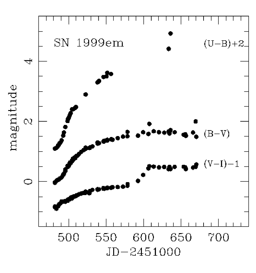
Figure 2: Color curves of SN 1999em.

Figure 2 shows some of the color curves of SN 1999em. They all reveal the reddening of the SN due to the cooling of its atmosphere. In $U-B$ and $B-V$ the reddening was more pronounced due to the many metal lines which depressed the SN flux at the wavelengths sampled by the $U$ and $B$ bands. The $V-I$ color, on the other hand, was less affected by line blanketing and better sampled the continuum emission. The evolution of SN 1999em in this color showed rapid cooling during the first 50 days, after which $V-I$ remained nearly constant for another $\sim$30 days. During this phase, the photosphere was near the hydrogen recombination surface and was then of nearly constant temperature (E96). The end of the plateau phase at JD 2451590 coincided with a sudden reddening of the SN, while the exponential tail was characterized by a nearly constant $V-I$ color.

2.2 Spectroscopy

We obtained optical and IR spectra of SN 1999em with the ESO NTT/EMMI at La Silla and VLT/ISAAC at Cerro Paranal between 1999 November 2 and November 28, and additional optical spectra with the CTIO 1.5-m telescope on October 30 (one day after discovery), and the SO Bok 2.3-m telescope and Boller & Chivens spectrograph on December 16 and December 31. Table 2 presents a journal of the observations.

2.2.1 Optical Spectroscopy

The NTT observations employed three different setups. We used the blue channel of EMMI equipped with a Tek CCD (1024x1024) and grating 5 (158 lines mm^-1) which, in first order, delivered spectra with a dispersion of 3.5 Å pix^-1 and a useful wavelength range between 3300 and 5250 Å. With the red channel, CCD Tek 2048, and grating 13 (150 lines mm^-1) the dispersion was 2.7 Å pix^-1 and the spectral coverage ranged from 4700 through 11000 Å in first order. Since this setup had potential second-order contamination beyond $\sim$6600 Å we decided to take one spectrum with the OG530 filter and a second observation without the filter, in order to provide an overlap with the blue spectrum. Thus, a single-epoch observation usually consisted of three spectra. On two occasions (November 3 and November 14) however, we were unable to obtain the observation with the OG530 filter, so the red end of the spectra were most likely contaminated by second-order blue light (more below).

The observations with EMMI started with calibrations during day time (bias and dome flat-field exposures). The night began with the observation of a spectrophotometric standard [from the list of Hamuy et al. (1994)] through a wide slit of 10 arcsec, after which we observed the SN with a slit of 1 arcsec. We took two exposures per spectral setup, each of the same length (typically 120-180 sec) and always along the parallactic angle. Immediately following this observation we observed a He-Ar lamp, at the same position of the SN and before changing the optical setup in order to ensure an accurate wavelength calibration. At the end of the night we observed a second flux standard.

We carried out all reductions using IRAF. They consisted in subtracting the overscan and bias from every frame. Next, we constructed a flat-field from the quartz-lamp image, duly normalized along the dispersion axis. We proceeded by flat-fielding all of the object frames and extracting 1-D spectra from the 2-D images. We followed the same procedure for the He-Ar frames which we used to derive the wavelength calibration for the SN. We then derived a response curve from the two flux standards, which we applied to the SN spectra in order to get flux calibrated spectra. During this process we also corrected for atmospheric extinction using an average continuum opacity curve scaled for the airmass at which we observed the object, but we did not attempt to remove telluric lines. From the pair of flux-calibrated spectra that we secured for each spectral setup we removed cosmic rays and bad pixels, and obtained a clean spectrum of the SN. The last step consisted in merging the three spectra that sampled different wavelength ranges. To avoid discontinuities in the combined spectrum we grey-shifted the three spectra relative to each other. Finally, we computed the synthetic $V$-band magnitude from the resulting spectrum (following the precepts described in Appendix B) and grey-shifted it so that the flux level matched our observed $V$ magnitude. We checked the spectrophotometric quality of the spectra by computing synthetic magnitudes for the $BRIZ$ bands. This test showed differences between the synthetic and observed magnitudes of up to 0.03 mag in the $B$ and $R$ bands, which implies that the relative spectrophotometry at these wavelengths was very good. The $I$ and $Z$ synthetic magnitudes, on the other hand, disagreed with the observed magnitudes by up to 0.1 mag, particularly when the blocking filter could not be used; second-order contamination was as large as 10% at those wavelengths.

We obtained a spectrum of the SN one day after discovery with the CTIO 1.5-m telescope and the Cassegrain spectrograph, a 1200x800 LORAL CCD, grating 16 (527 lines mm^-1) and 2 arcsec slit, in first order. The resulting spectrum had a dispersion of 5.7 Å pix^-1 and useful wavelength coverage of 3300-9700 Å. Second-order contamination was expected beyond 6600 Å due to first-order 3300 Å light since we did not use a blocking filter. On two nights we employed the SO Bok telescope with the Boller & Chivens spectrograph, a 1200x800 LORAL CCD, and a 300 lines mm^-1 grating which, in first order, produced spectra with a dispersion of 3.6 Å pix^-1. The wavelength coverage was 4900-9300 Å on December 16 and 3500-7100 Å on December 31. We did not include a blocking filter in the optical path, so it could well be that these spectra were affected by second-order contamination beyond 6600 Å. The observing and reduction procedures for the CTIO and SO spectra were the same as those described above for the NTT data.

Figure 3 displays the optical spectra in the rest-frame of the SN, after correcting the observed spectra for the 717 km s^-1 recession velocity of the host galaxy. The strongest SN lines are indicated along with the telluric lines (by the $\oplus$ symbol). The first spectrum, taken on JD 2451481.79 (1 day after discovery), showed a blue continuum with a $BVI$ color temperature of 15,600 K, P-Cygni profiles for the H Balmer lines, and the He I $\lambda$5876 line which is characteristic of SNe II during their hottest phases. The expansion velocity from the minimum of the absorption features was $\sim$10,000 km s^-1 which is typical of SNe II during the initial phases. The presence of the interstellar Na I D lines $\lambda\lambda$5890, 5896 with an equivalent width of $\sim$2 Å  suggested substantial interstellar absorption in the host galaxy. However, there is additional evidence that the SN did not suffer significant extinction (see Sec. 3.3) so we did not attempt to correct for dust the spectra of Figure 3.

As the SN evolved the atmospheric temperature dropped, the He I $\lambda$5876 line disappeared, and several new lines became evident, namely, the Ca II H&K $\lambda\lambda$3934,3968 blend, the Ca II triplet $\lambda\lambda$8498,8542,8662, the Na I D blend, and several lines attributed to Fe II, Sc II, and Ba II. Table 3 summarizes the line identifications, their rest wavelengths [taken from the list of Jeffery & Branch (1990)], and their wavelengths measured from the absorption minimum. We include several lines with unknown identifications in this table. By the time of our last spectrum on JD 2451543.76 (62 days after discovery) the $BVI$ color temperature was only 5,000 K, approximately the recombination temperature of H.

2.2.2 Infrared Spectroscopy

We obtained three IR spectra with the VLT/Antu telescope at Cerro Paranal, between November 2-28. We employed the IR spectro-imager ISAAC Moorwood (1997) in low resolution mode (R$\sim$500), with four different gratings that permitted us to obtain spectra in the $Z$, $J$, $H$, and $K$ bands. We used these gratings in 5^th, 4^th, 3^rd and 2^nd order, respectively, which yielded useful data in the spectral ranges 9840-11360, 11090-13550, 14150-18180, and 18460-25600 Å. The detector was a Hawaii-Rockwell 1024x1024 array.

A typical IR observation started during daytime by taking calibrations. We began taking flat-field images using an internal source of continuum light. We secured multiple on- and off-image pairs with the same slit used during the night (0.6 arcsec). We then took Xe-Ar lamp images (and off-lamp images) with a narrow slit (0.3 arcsec) in order to map geometric distortions. The observations of SN 1999em consisted in a O-S-O-S-O cycle, where O is an on-source image and S is a sky (off-source) frame. Given that the angular size of the host galaxy was comparable to the slit length (2 arcmin), it was not possible to use the classical technique of nodding the source along the slit and it proved necessary to offset the telescope by several minutes of arc to obtain the sky images. At each position we exposed for 200 sec, conveniently split into two 100-sec images in order to remove cosmic rays and bad pixels from the final spectra. After completing the O-S-O-S-O cycle we immediately obtained a pair of on-off arc lamp exposures without moving the telescope or changing optical elements to ensure an accurate wavelength calibration. We then switched to the next grating and repeated the above object-arc procedure until completing the observations with the four setups. For flux calibration we observed a bright solar-analog star, close in the sky to the SN in order to minimize variations in the atmospheric absorptions (Maiolino, Rieke, & Rieke 1996). The selected star was Hip 21488, of spectral type G2V, $V$=8.5, $B-V$=0.6, and located only 12^∘ from the SN (SIMBAD Astronomical Database). In this case we nodded the object between two positions (A and B) along the slit and we took two AB pairs for each grating. To avoid saturating the detector, we took the shortest possible exposures (1.77 sec) allowed by the electronics that controlled the detector. Since the minimum time required before offsetting the telescope was $\sim$60 sec, we took ten exposures at each position which provided an exceedingly good signal-to-noise ratio (S/N) for the flux standard.

The reductions of the IR data began by subtracting the off-lamp images from the on-lamp flat-field frames, median filtering the multiple flat images, and normalizing the resulting frame along the dispersion axis. Then we divided all of the object images by the normalized flat-field. The next step consisted in mapping the geometric distortions using the arc lamp taken with the narrow slit. The emission lines displayed a curvature of a few pixels across the spatial direction of the image. From the narrow-slit arc exposure we obtained sharp emission lines which allowed us to form a 2-D map of the distortions. We then fit a low-order 2-D polynomial to the line tracings, after which we applied a geometric correction to all of the images obtained during the night. Since the sky background is so large in the IR, a small flat-fielding residual or a patchy sky can introduce large background fluctuations. This made it necessary to subtract the sky from the 2-D images before attempting to extract the object spectrum. Given that the IR sky changes on short time-scales, we always used the sky image taken immediately before or after the SN frame. We followed the same procedure for the flux standard. We then extracted 1-D spectra of the SN and the spectrophotometric standard from the sky-subtracted frames, making sure to subtract residual sky from a window adjacent to the object. We also extracted a spectrum of the Xe-Ar frame taken at the same position of the SN, in order to derive a wavelength calibration. We then combined the multiple spectra of the SN and the standard with a ‘minmax’ rejection algorithm that removed deviant pixels from the average at each wavelength.

Flux calibration in the IR is in general quite involved because there are no flux standards at these wavelengths. To get around this problem we adopted the technique described by Maiolino et al. (1996), which consists in dividing the spectrum of interest by a solar-type star to remove the strong telluric IR features, and multiplying the resulting spectrum by the solar spectrum to eliminate the intrinsic features (pseudonoise) introduced by the solar-type star. In its original version this method used a solar spectrum normalized by its continuum slope, so the object’s spectrum was not properly flux calibrated. More recently (http://www.arcetri.astro.it/$\sim$maiolino/solar/solar.html) this technique was modified to incorporate a flux-calibrated semi-empirical spectrum of the Sun, so that the object’s final spectrum is in flux units. The adopted spectrum is a combination of the observed solar line spectrum in the $JHK$ bands Livingston & Wallace (1991) and the Kurucz solar model with parameters $T_{eff}$=5,777 K, log $g$=4.4377, [Fe/H]=0, $V_{microturb}$=1.5 km s^-1 Kurucz (1995). In the Vega magnitude system (described in Appendix B), the solar spectrum has a visual magnitude of -26.752. The remaining broad-band magnitudes are listed in Table 12.

Before using the solar spectrum we convolved it with a kernel function in order to reproduce the spectral resolution of the solar-analog standard Hip 21488, and we scaled it down to the equivalent of $V$=8.5 which corresponds the the observed magnitude of Hip 21488. From the ratio of this solar spectrum and the observed spectrum of Hip 21488 we derived an instrumental response curve which included both the telluric absorption lines and the instrumental sensitivity of ISAAC. Finally, we multiplied the SN spectrum by the response function to obtain the flux-calibrated SN spectrum. This technique worked very well to remove telluric lines. On the other hand, it introduced a small systematic error in the flux calibration of the SN due to departures between the solar spectrum and the actual spectral energy distribution of the solar-analog standard. According to atmosphere models the difference in continuum flux for stars with $T_{eff}$=5,500 and 6,000 K (which correspond to spectral types G8V-F9V, Gray & Corbally 1994) is smaller than 10% in the NIR region. A G2V star like Hip 21488 has the same spectral type of the Sun, so its effective temperature must be close (within $\pm$100 K) to that of the adopted solar model. Hence, the flux difference between the solar-analog standard and the adopted spectrum should be less than 10%. The $B-V$=0.6 color of Hip 21488 suggests little or no reddening so the SN spectra fluxes are probably accurate to 5% or better.

The result of these operations are four spectra covering the $Z$, $J$, $H$, and $K$ bands, which we combined into one final spectrum. Given the significant overlap of the $Z$ and $J$ band spectra, we were able to grey-shift the $Z$ spectrum relative to the $J$ spectrum. Since none of the other spectra overlapped (due to the strong absorption of telluric lines between the $J$, $H$, and $K$ bands), we shifted them individually by computing synthetic magnitudes (see Appendix B) and bringing them into agreement with the observed photometry.

Figure 4 shows the resulting rest-frame spectra of SN 1999em, revealing the exquisite spectral resolution and the superb S/N delivered by ISAAC. The first spectrum, taken four days after discovery, showed a few prominent lines, namely He I $\lambda$10830, P$\alpha$, P$\beta$, B$\gamma$, and B$\delta$, on top of a blue continuum. The second spectrum (20 days after discovery) showed prominent P$\gamma$ and P$\delta$ lines in lieu of the strong He I feature. A few faint lines appeared around 17000 Å, from higher transitions in the Brackett series. The third spectrum, taken 30 days after discovery, confirmed the presence of these faint lines. Three lines could be seen at $\sim$10500 Å , between P$\gamma$ and P$\delta$. It is possible that the feature at 10180 Å was due to the 10327 Å line of the multiplet 2 of Sr II, which was also observed in SN 1987A Elias et al. (1988). The other two lines of the multiplet at 10037 and 10915 Å  were probably blended with P$\delta$ and P$\gamma$, respectively. We cannot provide identifications with confidence for the other two features at 10418 and 10549 Å . Meikle et al. (1989) identified the C I $\lambda$10695 multiplet 1 line in an early-time spectrum of SN 1987A, which might be responsible for the 10549 Å  feature in the SN 1999em spectrum. They also reported the presence of the He I $\lambda$10830 absorption line in late-time spectra of SN 1987A. It is possible then that the 10418 Å feature in SN 1999em could be due to He I. Table 4 summarizes the line identifications, their rest wavelengths and the values measured from the absorption minima.

Given that two of the IR spectra were obtained one day apart from the optical spectra, we were able to combine these observations in Figure 5. This exercise revealed the excellent agreement between the optical and IR fluxes, a result made possible by synthesizing broad-band magnitudes and adjusting the flux scales according to the observed magnitudes. Second-order contamination can be clearly seen in the first-epoch spectrum as a flux excess between 7500-10000 Å.

3 THE APPLICATION OF THE EXPANDING PHOTOSPHERE METHOD TO SN 1999em

EPM involves measuring a photometric angular radius and a spectroscopic physical radius, from which the SN distance can be derived. In this section we apply the method to SN 1999em following such order. In Appendix A we summarize the basic ideas behind EPM.

3.1 The angular radius of SN 1999em

The angular radius, $\theta$, of the SN can be determined from equation A1 by fitting Planck curves [$B_{\lambda}(T_{S})$] to the observed magnitudes. With two wavelengths the solution is exact (two equations and two unknowns). For three or more wavelengths we use the method of least-squares at each epoch to find the color temperature $T_{S}$ and the parameter $\theta\zeta_{S}$ that minimize the quantity

$$\chi^{2}=\sum_{\overline{\lambda}~{}\epsilon~{}S}\frac{[m_{\overline{\lambda}}~{}+5~{}log~{}(\theta\zeta_{S})~{}-~{}b_{\overline{\lambda}}(T_{S})]^{2}}{\sigma_{m}^{2}}.$$ (1)

In this equation $m_{\overline{\lambda}}$ is the SN’s apparent magnitude in a photometric band with central wavelength ${\overline{\lambda}}$, $\sigma_{m}$ is the corresponding photometric error, $b_{\overline{\lambda}}(T_{S})$ is the synthetic magnitude of $\pi B_{\lambda}(T_{S})10^{-0.4A(\lambda)}$ (computed with the precepts described in Appendix B), and $A({\lambda})$ is the dust extinction affecting the SN. Once $\theta\zeta_{S}$ is determined from the $\chi^{2}$ fit, we solve for $\theta$ using the dilution factor $\zeta_{S}$ corresponding to filter subset $S$, which we compute from the color temperature using equation C2.

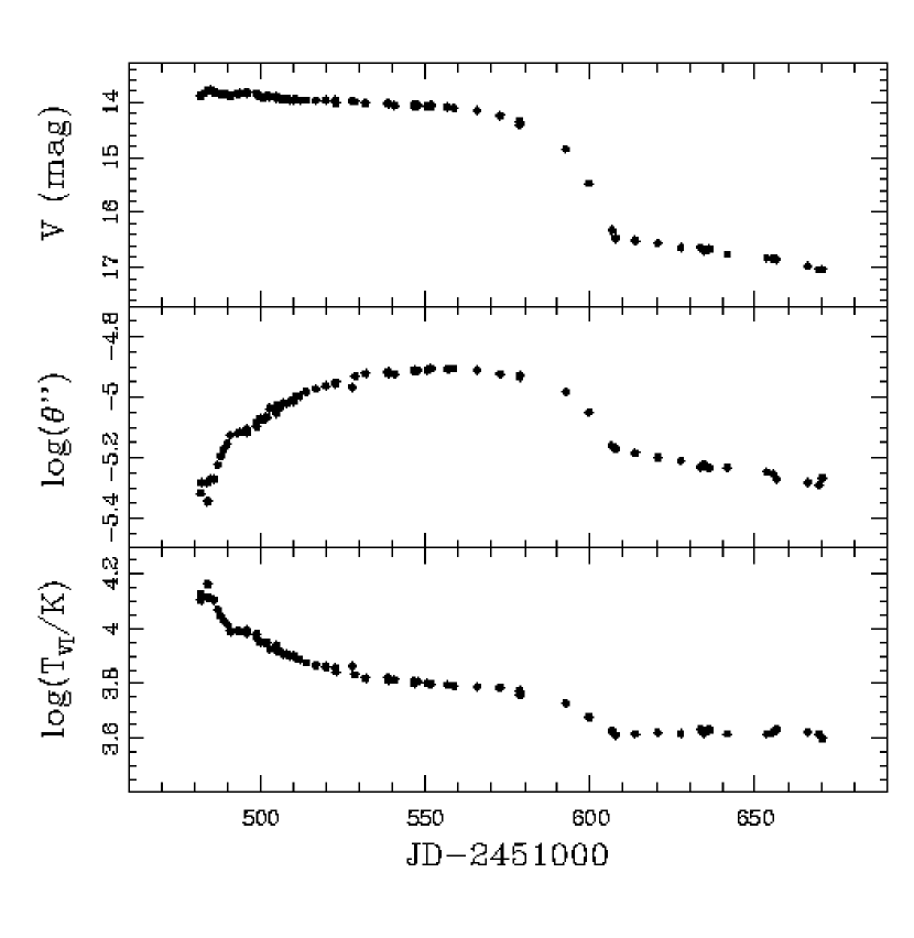
Figure 6: $V$ magnitude, photospheric angular radius, and color temperature of SN 1999em vs. Julian Day.

Using the $VI$ photometry and adopting a foreground extinction of $A_{Gal}(V)$=0.13 (Schlegel, Finkbeiner, & Davis 1998) and $A_{Host}(V)$=0.18 for dust absorption in the host galaxy Baron et al. (2000), we compute $T_{VI}$ and the corresponding angular radius, which are plotted in Figure 6. This figure shows that the initial color temperature was $\sim$13,000 K and that the SN cooled down for nearly 60 days until reaching a value near 6,500 K. The photosphere remained at this temperature for 30 days more until the end of the plateau phase. In the rapid fall off the plateau, the atmosphere cooled to $\sim$4,000 K after which the temperature remained nearly constant. At this stage the SN began the nebular phase and the spectrum was dominated by recombination lines so the color temperature cannot be associated with a thermal process. During the initial cooling period of 60 days the photospheric radius steadily increased as the photosphere was swept outward by the expansion of the ejecta, and then decreased as the wave of recombination moved into the flow with ever-increasing speed. It is this balance between increasing radius and steady cooling which explains the long plateau of nearly constant luminosity (top panel). Following the plateau phase, both the radius and the temperature decreased, leading inevitably to the luminosity drop around day JD 2451580.

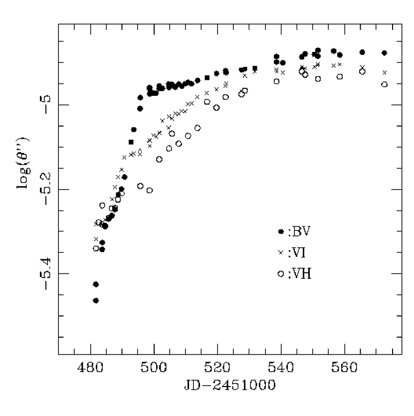
Figure 7: Photospheric angular radius of SN 1999em derived from filter subsets $\{BV,VI,VH\}$, as a function of time.

Since the radiation field forms at a depth which varies with wavelength (depending on the value of the absorptive opacity), the angular radii derived before corrections for the dilution factors are expected to vary significantly depending on the filters employed in the blackbody fits. By contrast, the photosphere is defined as the region of total optical depth $\tau$=2/3, the last scattering surface. Since continuum opacity in the optical and NIR is dominated by electron scattering, the opacity is grey, and the photospheric angular radius is not expected to change with wavelength (E96). We can check this prediction in Figure 7 by comparing the photospheric angular radii derived from filter subsets $\{BV,VI,VH\}$ for the entire plateau phase of SN 1999em. The relative agreement is excellent ($<$5%) over the first 10 days of SN evolution, after which there is a period of $\sim$30 days in which the photospheric radii derived from the three filter subsets disagree by up to 25%. Over the following 60 days the agreement is much better, at the level of 10%. This test reveals the overall good agreement of the photospheric radii determined from different filters and the good performance of the dilution factors.

3.2 The physical radius of SN 1999em

The next step in deriving an EPM distance involves the determination of photospheric velocities from the SN spectra. To date the photospheric velocities have been estimated from the minimum of spectral absorption features (Schmidt et al. 1992, 1994). There are several problems with this approach, however. First, the location of the line minimum shifts toward bluer wavelengths (higher velocity) as the optical depth of the line and the scattering probability increase. This is a prediction of line profile models in homologously expanding scattering atmospheres [see Fig. 3 of Jeffery & Branch (1990), for example], and is also an observational fact as Figure 8 demonstrates. This plot shows the expansion velocities derived from the metal (Sr, Ca, Fe, Na, Si) lines of the spectrum taken on 1999 December 31, as a function of the equivalent width of the line. Even though it proves difficult to measure line strengths due to the lack of a well-defined continuum, the trend is quite evident in the sense that stronger features yield higher velocities. It is well known that hydrogen lines (which are not shown in this plot) yield much higher expansion velocities than the metal lines in SN II spectra due to their high optical depths, but no attention has yet been paid to this effect among the weakest absorptions. This plot shows that it is possible to incur significant errors if we measure expansion velocities from the minima of absorption features, even from the weakest lines. Second, even if we could extrapolate the observed velocities to zero strength, the inferred velocity would correspond to that of the thermalization surface (where the radiation field forms) and not to the photosphere (the last scattering surface). Since the dilution factors computed by E96 correspond to the ratio of the luminosity of the SN model to that of a blackbody with the photospheric radius of such model (see Appendix C), the use of the velocity of the thermalization surface is inappropriate, even though it has been common practice in the past. Third, velocities derived from absorption lines are affected by line blending or possible line misidentifications, both of which can lead to an erroneous estimate of the photospheric velocity.

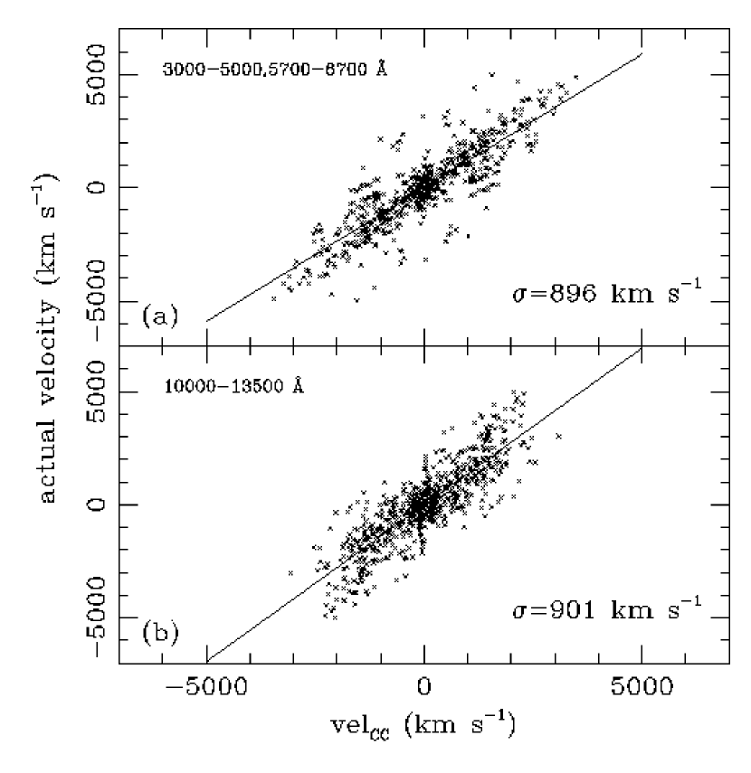
Figure 9: (a) Relative expansion velocities derived from the cross-correlation technique for pairs of model spectra with similar color temperatures, versus the actual relative velocities. The cross-correlation was restricted to the range 3000-5000, 5700-6700 Å. (b) Same as (a) but for the range 10000-13500 Å.

To get around these problems we adopt an approach based on cross-correlating the SN spectrum with the models of E96 (with known photospheric velocities) using the IRAF “fxcor” task. Before applying this technique to the observed spectra, we must test it with the model spectra of E96. In doing so we cross-correlate models with other models having $BVI$ color temperatures within $\pm$1,000 K of each other. For each pair of models we end up with a relative velocity derived from the cross-correlation (CC, hereafter) technique which can then be compared with the actual value. The hope is that the whole set of pairs can be used to derive a relationship between the CC relative velocity and the actual value. We carry out tests separately in the optical and the IR in order to apply this method to spectra observed in different spectral windows. In the optical we select two wavelength ranges (3000-5000, 5700-6700 Å) and a NIR a window between 10000-13500 Å. We end up with these ranges after numerous experiments which show that beyond 13500 Å there are too few spectral lines to help us constraining the expansion velocity. In the optical these tests suggest us to eliminate the red wings of the strong H$\alpha$ and H$\beta$, which have the potential to bias the derivation of expansion velocities from the CC procedure. Figure 9 compares the CC relative velocities and the actual values, both in the optical and NIR, from the whole set of models (except for s15.5.1 and s25.5.1 which are not appropriate for SNe II-P, E96). In both cases we get a reasonable correlation which permits us to convert the velocity offsets measured from cross-correlation into a photospheric velocity. The scatter in these relationships is 900 km s^-1 which provides an estimate of the precision in the derivation of a photospheric velocity from a single model. The data can be adequately modeled with straight lines, both in the optical and IR. Least-squares fits yield slopes of 1.18 in the optical and 1.38 in the NIR, and zero-points of -3 km s^-1 in both cases. This implies that the magnitude of the relative velocity is smaller than the actual value. Overall, this is an encouraging result, although it must be mentioned that the points with the largest scatter in Figure 9 correspond to pairs with the largest temperatures. This means that the precision of the CC technique drops to $\sim$2000 km s^-1 when $T_{BVI}$$>$8,000 K.

Having come up with a method to estimate photospheric expansion velocities we can proceed to derive velocities for SN 1999em. We start by selecting atmosphere models with $BVI$ color temperatures within $\pm$1,000 K of each observed spectrum, after which we cross-correlate the SN spectrum and the subsample of models in the aforementioned wavelength windows. The outcome of this operation is a cross-correlation function (CCF) with a well-defined peak whose location in velocity space gives the relative velocity of the observed and reference spectrum. The height of the CCF is a measure of how well the spectral features of the two spectra match each other. Figure 10 shows examples of the CC technique. Panel (a) compares the optical spectrum obtained on JD 2451501.66 (thick line) with four models of similar color temperature (thin lines), and panel (b) shows the corresponding CCFs. The two models that best match the observed spectrum, p6.60.1 and p6.40.2, are the ones that give the highest CCF peaks. Models s15.43.3 and s15.46.2, on the other hand, provide poorer matches to the observed spectrum and, consequently, the lowest CCF peaks. For each cross-correlation we get a relative velocity which we proceed to correct using the calibrations shown in Figure 9, in order to get the actual relative velocity. Since the photospheric velocities of the models are known, we can derive independent photospheric velocities for each SN spectrum. Table 5 summarizes the velocities derived with this method for all of the spectra of SN 1999em. In this table $v_{CC}$ is the relative velocity determined from the CC method, $v_{model}-v_{SN}$ is the actual relative velocity derived from the calibration provided by the straight lines in Figure 9, and $v_{SN}$ is the photospheric expansion velocity of the SN. Note that, for a given epoch, the expansion velocities derived from different models agree quite well. Table 6 presents the average velocity obtained for each epoch along with the rms value derived from the different models. Note the great agreement in the photospheric velocities determined from optical and IR wavelengths. While the lines used in the different spectral regions form at different depths, the CC technique yields photospheric velocities that do not depend on the wavelength region employed in the cross-correlation, which is the expected behavior for the photosphere. Inspection of Table 6 shows that the scatter in velocity yielded by multiple cross-correlations varies between 5-21%. The errors in the average velocities are probably smaller than the tabulated values because we make use of various models to compute such averages.

For comparison we include in Table 6 velocities determined from the conventional method of measuring the wavelength of weak absorption lines. Following the approach of Schmidt et al. (1994), we list velocities measured from Fe II $\lambda$5018 and Fe II $\lambda$5169 ($v_{Fe}$), and from Sc II $\lambda$5526 and Sc II $\lambda$5658 ($v_{Sc}$). We include also estimates from all metal lines but the strong calcium features ($v_{lines}$). This comparison shows that $v_{lines}$$\sim$$v_{Fe}$$>$$v_{Sc}$. While $v_{Fe}$ and $v_{Sc}$ have low internal errors when considered individually, the average derived from multiple weak lines displays considerable scatter. This demonstrates that the technique of using a few pre-selected weak absorption lines has the potential to produce very different results, so that the internal precision of the Fe or Sc method must reflect the velocity scatter yielded by all lines, which is $\sim$20%. Figure 11 shows a comparison between the velocities derived from measuring the weak metal lines and the CC method. During the first 15 days, line velocities are $\sim$20% lower than the CC velocities, after which this difference becomes negligible. In our last-epoch spectrum, on the other hand, there is a hint that the velocity derived from absorption lines is higher than that obtained from the CC method, although the difference amounts to only $\sim$1$\sigma$.

3.3 The distance to SN 1999em

In this section we use EPM to derive the distance to SN 1999em. In doing so we adopt the foreground extinction $A_{Gal}(V)$=0.13 measured by Schlegel et al. (1998). The presence of interstellar Na I D in the SN spectrum at the wavelength corresponding to the velocity of the host galaxy with an equivalent width of $\sim$2 Å suggests that additional reddening affected the SN. According to the correlation between equivalent width and reddening of Munari & Zwitter (1997), SN 1999em was reddened by $E(B-V)$_host$\sim$1.0$\pm$0.15. This estimate is highly inconsistent with the independent estimate of $E(B-V)$_host$\approx$0.01-0.06 and $E(B-V)$_host$<$0.11 from theoretical modeling of the spectra of SN 1999em (Baron et al. 2000) . This disagreement suggests that the light of SN 1999em was likely absorbed by a gas cloud with relatively large gas to dust ratio, perhaps ejected by the supernova progenitor in an episode of mass loss. This example demonstrates the difficulty of using the equivalent width of interstellar lines to estimate dust extinction due to the uncertainty in the calibration. Another example that illustrates the problem of applying the Galactic calibration of Munari & Zwitter to SNe is the highly reddened Type Ia SN 1986G. The spectra of this SN revealed interstellar Na I D absorption with an equivalent width of 4.1 Å Phillips et al. (1987) which implies $E(B-V)$$\sim$2, yet the reddening yielded by color considerations was $E(B-V)$=0.62 Phillips et al. (1999).

In what follows we examine the sensitivity of EPM to dust for which we adopt a wide range of extinction values between $A_{Host}(V)$=0-0.45 mag. Figure 12 shows the EPM distances derived for eight filter subsets (from $B$ through $K$). This plot reveals that the distance from subset {$BV$} decreases from 7.4 to 6.2 Mpc when the adopted extinction increases from 0 to 0.45 mag. A similar behavior can be appreciated from filters {$BVI$}. From {$VI$} we find that the distance changes only from 7.6 to 7.0 Mpc, i.e., EPM is very insensitive to our choice of $A_{Host}(V)$ when observing with these filters. This trend reverses with subsets including the IR filters, i.e., the distance gets bigger as the adopted extinction increases. This plot shows empirically that the EPM distances are quite robust to the effects of extinction. The other interesting feature of this plot is that these curves show a convergence toward small values of $A_{Host}(V)$, which allows us to constrain the value of the extinction in the host galaxy. In what follows we adopt $A_{Host}(V)$=0.18 which is the most likely value derived by Baron et al. (2000) and, as Figure 12 shows, is also consistent with the EPM analysis.

Tables 7-10 summarize the EPM quantities derived for SN 1999em using eight filter subsets. The photospheric velocities come from the polynomial fit to the velocities obtained from the CC technique (the solid line in Figure 11), to which we assign a statistical uncertainty of 5%. The color temperature $T_{S}$ and the quantity $\theta\zeta_{S}$ correspond to parameters obtained from the $\chi^{2}$ minimizing procedure described in Sec. 3.1 (equation 1), which allows us to estimate statistical uncertainties in the derived parameters from the photometric errors. Also listed in these tables is the dilution factor $\zeta_{S}$ required for the derivation of the $(\theta/v)_{S}$ quantity needed for EPM. In the models of E96, this factor is primarily determined by temperature and, for a given temperature, $\zeta_{S}$ changes only by 5-10% over a large range of other parameters. This is a remarkable result, permitting us to compute $\zeta_{S}$ for SN 1999em without having to craft specific atmospheric models. Using this approximation and the derived color temperature, we compute $\zeta_{S}$ from the polynomial fits to the dilution factors for our photometric system (Appendix C; equation C2). With this approach we expect a component of systematic error ($\sim$5-10%) in $(\theta/v)_{S}$. Since this is not a statistical uncertainty, we do not include it in the error quoted for $(\theta/v)_{S}$ in Tables 7-10.

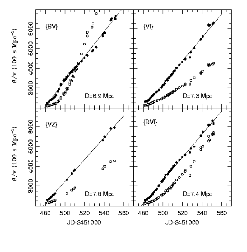
Figure 13: $\theta$/$v$ as a function of time for filter subsets $\{BV,VI,VZ,BVI\}$. Open dots show $\theta$$/v$ uncorrected for dilution factor while filled dots show the parameter corrected with the factors computed by E96. In theory, this quantity should increase linearly with time and the slope of the relation gives the distance (Appendix A). The small departures of these points from the ridge lines demonstrate the good performance of the dilution factors at different times over a broad wavelength range.

Figure 13 shows $\theta$$/v$ as a function of time, for four subsets including filters $B$ through $Z$. The open dots show $\theta/v$ uncorrected for dilution factors while the filled dots show the parameter after correction. In theory, $\theta/v$ should increase linearly with time (except for the very first days after explosion) and the slope of the relation gives the distance (equation A4). Overall, this figure reveals that the dilution factors produce distances with reasonable consistency during a period of 70 days of SN evolution in which the photospheric temperature dropped from 15,000 to 5,000 K, although it is evident that there are systematic departures from linearity. In particular, the earliest points provide evidence that the angular radius is too large relative to the physical size implied by homologous expansion of the photosphere from a point. This suggests that the progenitor’s radius ($R_{0}$) might have a non-negligible contribution to the SN radius in the first observations (obtained a few days after shock breakout). A week after explosion $R_{0}$ becomes negligible, even for the largest red supergiants known ($R_{0}$=300$R_{\odot}$, van Belle et al. 1999), so its effect in the determination of the distance can be ignored. Hence, we proceed now to fit the data with a straight line using equation A4, and in the next section we review the validity of this approximation.

To compute the distance it suffices, in principle, to perform a least-squares fit to the ($\theta_{i}/v_{i}$,$t_{i}$) points. To perform such fit it is necessary to know the uncertainty in each of the $\theta_{i}/v_{i}$ points. In our case this is rendered difficult by our lack of knowledge of the systematic errors in $\zeta_{S}$ which is needed to obtain the $\theta/v$ parameter. By weighting the fits by the errors, the fits are going to be biased significantly to the earlier data which carry a lot of weight. Equal weighting seems to be a more reasonable way to derive an “average” distance. To estimate the uncertainties in the distance and explosion time we employ the bootstrap technique described by Press et al. (1992) which makes use of the data themselves as an estimator of the underlying probability distribution (which we do not know). The method consists in randomly drawing from the parent population a synthetic dataset of the same size as the parent. By drawing points with replacement we end up with a randomly modified dataset, from which we perform a uniform-weight least-squares fit in order to solve for the time of explosion $t_{0}$ and the distance $D$. From a large number (10,000) of simulations we obtain average parameters and estimates of the uncertainties in $t_{0}$ and $D$ from the dispersion among the many bootstrap realizations.

The ridge lines in Figure 13 correspond to the solutions determined from the bootstrap method and the results of the fits are given in Table 11. The range in distance (6.9-7.8 Mpc) derived from observing through these four filter subsets is quite small ($\pm$6%). This shows the good performance of the dilution over the broad wavelength range encompassed by the $BVIZ$ filters. The nominal error yielded by the bootstrap method for the individual subsets ranges between 1-2%, which proves significantly smaller than the 6% distance range encompassed by the four subsets. Most likely, this is a symptom of systematic errors in the dilution factors.

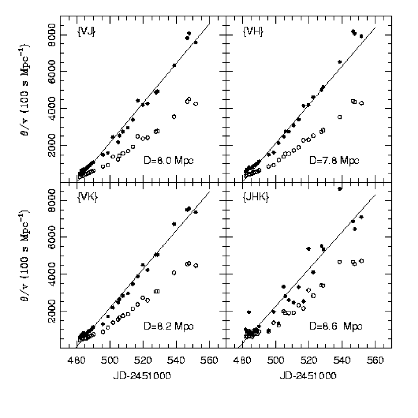
Figure 14: Same as Figure 13, but for filter subsets $\{VJ,VH,VK,JHK\}$.

Figure 14 shows $\theta$$/v$ as a function of time from filter subsets including IR wavelengths. The scatter from the ridge line is somewhat higher than that obtained from optical wavelengths due to the relatively larger photometric errors in the IR. This problem becomes even stronger for the $\{JHK\}$ subset because the errors in the derived color temperatures increase as the Rayleigh-Jeans limit is approached. Despite the larger scatter in the distances derived from IR observations, this plot confirms the internal consistency of the dilution factors computed by E96 from IR wavelengths. The fits to the data are listed in Table 11 which shows that the resulting distances are quite consistent with those derived from optical observations, although the differences are somewhat larger than the formal errors (more below).

We include also in Table 11 a solution derived from a simultaneous least-squares fit to all of the $(\theta/v)_{S}$ values in Tables 7-10. Not surprisingly, the resulting distance of 7.54 Mpc is close to the value of 7.75 Mpc obtained from taking a straight average of the eight individual distances. We prefer the former estimate because it weighs the distances of the individual subsets according to their time sampling of the $(\theta/v)_{S}$ parameter. Also given in Table 11 is the distance of 7.82 Mpc determined from subset $\{BVIJHK\}$. In this case we must restrict the sample of $(\theta/v)_{BVIJHK}$ values to those epochs in which we obtained simultaneous observations with all six filters. Thus, the solution is not weighted by the higher frequency of the optical observations so the result is very close to the value of 7.75 Mpc obtained by averaging the individual distances yielded by the eight subsets. In what follows we adopt the value of 7.54 Mpc which takes into account the better sampling of the optical light curves.

The values derived for the explosion time are listed in Table 11. The average from the eight filter subsets is JD 2451478.8 ($\pm$1 day). This confirms that the SN was caught at a very young stage and that our first photometric and spectroscopic observation was obtained at an age of only three days after shock breakout. This is far earlier than any other SN, except for SN 1987A.

4 DISCUSSION

One of the challenges of EPM involves the determination of photospheric velocities. The spectra of SN 1999em show that the technique of cross-correlating the SN spectra with the models of E96 can produce expansion velocities with an average uncertainty of 11%. This is significantly lower than the 20% precision yielded by the method of measuring velocities from the minimum of weak absorption features (Table 6). The cross-correlation technique is not only more precise, but also more accurate, since the velocity derived from individual lines tend to correspond to the value of the thermalization surface, which expands more slowly than the photosphere (the last scattering surface). A clear advantage of the CC method is that it can be used during the initial hot phases of SN evolution when no weak lines are available. The other advantage of the CC technique is that it permits one to estimate velocities from lower S/N spectra, thus extending the potential of EPM to high redshifts where high-quality spectra are difficult to obtain.

The effects of dust extinction can seriously hamper the determination of distances when using “standard candle” techniques. EPM, on the other hand, is quite robust to the effects of dust absorption as pointed out by E96 and by Schmidt et al. (1992, 1994). While extinction reduces the observed flux, it also makes the photosphere appear cooler and hence less luminous, so that these two effects cancel to a significant degree. The data of SN 1999em provide empirical confirmation that the EPM distance to this SN is not very sensitive to the adopted absorption. We find that while the EPM distances derived from optical colors decrease with increasing $A_{Host}(V)$, this trend reverses when using IR filters (Figure 12). This analysis reveals that, even though IR photometry is less affected by dust, the EPM distances derived from filter subsets including one or more IR filters are not less sensitive to dust than those determined from optical filters alone. This result challenges the suggestion of Schmidt et al. (1992), namely, that one of the advantages of using IR for EPM is that “the uncertainty in a distance due to extinction is less than half that incurred when optical photometry is used”. Our analysis shows that the {VI} and {VZ} subsets have the least sensitivity to the effects of dust. In particular, the distances derived with the {VI} filters vary by a mere 7% when the adopted absorption is varied in a wide range of values between 0-0.45 mag. The other interesting result is that, despite the weak sensitivity of EPM to dust, multi-color observations can be useful for constraining $A_{Host}(V)$.

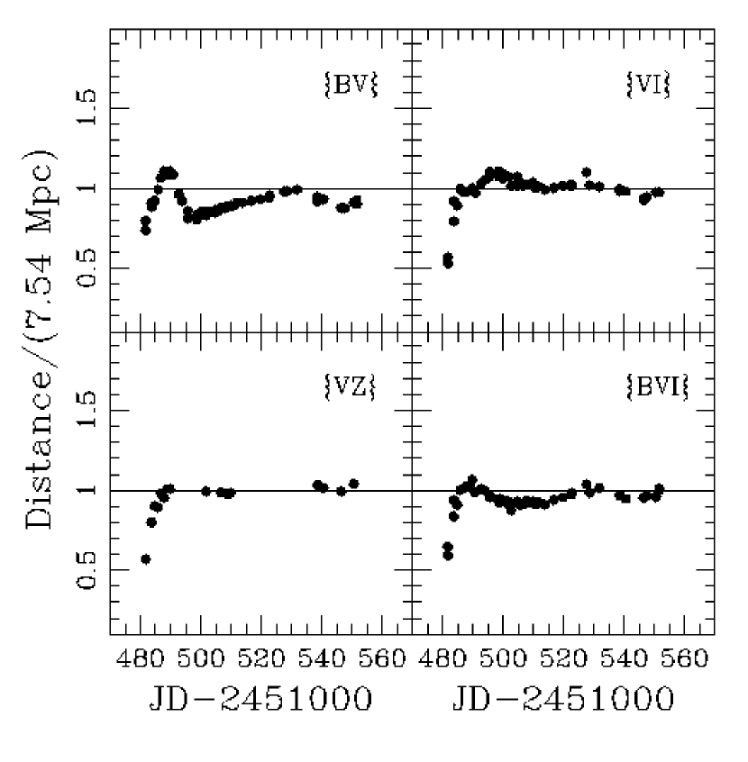
Figure 15: EPM distance as a function of time, for filter subsets $\{BV,VI,VZ,BVI\}$.

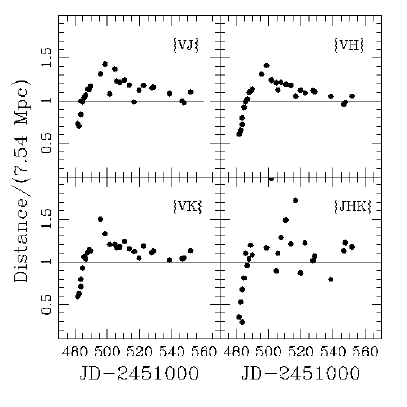
Figure 16: Same as Figure 15, but for filter subsets $\{VJ,VH,VK,JHK\}$.

EPM has the great advantage that observations at different epochs are essentially independent distance measurements. The exceptional data obtained for SN 1999em afford a unique opportunity to perform this valuable internal check and test the dilution factors of E96 over a wide range in temperature and wavelength. Figures 15 and 16 show that the EPM distance (in units of the average value of 7.54 Mpc obtained from the eight filter subsets) varies systematically over time (the error of one point is highly correlated to the error in the next point). This problem is particularly pronounced over the first week since explosion (JD 2451478.8), in which the distances prove even 50% lower than the average owing to the large photometric angular radius relative to the physical size of the SN. There are different possible causes for this discrepancy which we proceed to examine. The high degree of correlation in the errors derived from the different filter subsets suggests that the small linear radius might be due to an underestimate of the photospheric velocity. If this was the case the expansion velocity in the first observation epoch (JD 2451481.79) would have to be 50% higher than the adopted value. This is well beyond the $\sim$5% uncertainty in the CC technique, so we can rule out errors in the photospheric velocities as the source of this discrepancy. Another possible cause for the large initial distance residuals is the neglect of the initial radius $R_{0}$ in the linear size of the SN. To examine this issue in detail, Figure 17 shows how $\theta/v$ changes with time in a log-log scale, for the eight filter subsets. Overplotted are the lines corresponding to homologous expansion (equation A3) for the case of a progenitor with $R_{0}$=0 (solid line) and $R_{0}$=5$\times$10¹³cm (dotted line), which is 2$\times$ larger than the largest supergiant known van Belle et al. (1999). It is evident that the two models are almost identical at later times (when the effects of $R_{0}$ in the SN radius become negligible), and that they both fit the data very well after day 7. The earliest points, on the other hand, all fall on the high side of the lines of homologous expansion. This plot shows that, while the initial radius of the SN progenitor can account for some of the high $\theta/v$ values observed at the earliest epochs, there must be other reasons to explain the relatively large angular size of the SN. We cannot rule out, of course, that the large initial residuals are due to incorrect dilution corrections which would act to increase the derived values of $\theta$. For this to be true, the dilution corrections for all filter subsets should be increased by 2$\times$. It is conceivable that such error could be caused by circumstellar material which could lead to the formation of the photosphere at a much larger radius. This is an interesting possibility that could be clarified with an expanded set of atmosphere models for SNe II.

Leaving aside the origin of the high initial distance residuals it is interesting to ask what is their effect in the derived distance to SN 1999em. For such purpose we employ equation A3 to solve simultaneously for $R_{0}$, $t_{0}$, and $D$. A least-squares fit to the data, however, yields a degenerate and non-physical solution for the three parameters, most likely caused by the large residuals of the earliest points which demand an extremely large $R_{0}$. If, instead, we fix $R_{0}$ to the value of a very large progenitor, 5$\times$10¹³cm, we obtain a modest increase of 4% in the distance. Alternatively, we now ask what would be the distance if we exclude the first observations. Limiting the dataset to epochs later than JD 2451485.7 (one week after explosion), a linear fit yields $D$=7.40$\pm$0.09 Mpc and $t_{0}$=2451479.7$\pm$0.5, which are indistinguishable than the values derived from the entire dataset.

After day 7 (JD 2451485) the scatter in the EPM distances is much lower: 9% in $\{BV\}$, 4% in $\{BVI\}$, 4% in $\{VI\}$, and 4% in $\{VZ\}$. Inspection of Figure 15 shows that the residuals vary systematically over time. If these were caused by the adopted velocity the effect would be the same in the different filter subsets, which is not the case. We believe, instead, that the problem lies in the derived photospheric angular radii. In fact, Figure 7 reveals discrepancies of up to 10% in the values of $\theta$ obtained from different filter subsets. It could well be that these residuals are caused by the use of average dilution factors which, according to E96, have errors between 5-10%. Systematic errors in the photometry could also explain the discrepancies in $\theta$. Although the nominal uncertainties due to photon statistics are $\sim$0.015 mag, the transformation of instrumental magnitudes to the standard system could have significant systematic errors owing to the non-stellar nature of the SN spectrum Hamuy et al. (1990). In the IR the rms in the EPM distances after day 7 are 10% in $\{VJ\}$, 10% in $\{VH\}$, 9% in $\{VK\}$, and 27% in $\{JHK\}$. In theses cases the observational uncertainties are partially responsible for these relatively greater spreads, although it is evident that the EPM distances are systematically higher than the average and that they decrease steadily with time. We believe that this trend could be caused by systematic errors in the dilution factors or the photometry.

The distance residuals shown in Figures 15 and 16 reveal the potential problem of applying EPM to SNe II with small time baseline light curves. To illustrate this point we compute distances for SN 1999em using the data subset comprising the first days of SN evolution (up to JD 2451490), which yields $D(BV)$=10.34, $D(VI)$=9.70, $D(BVI)$=10.24, $D(VZ)$=9.95, $D(VJ)$=13.26, $D(VH)$=13.98, $D(VK)$=14.46, and $D(JHK)$=20.78 Mpc. Note that these distances are much higher than the 7.54 Mpc average value, whereas Figures 15 and 16 show that the EPM distances in the first week are on the low side from the average! This difference turns out to be a consequence of the shallower slope displayed by the early-time points in Figures 13 and Figures 14. A shallower slope implies a greater distance (equation A4), despite the fact that the individual points imply smaller distances owing to their relatively larger photospheric angular radii. This test reveals that a “snapshot” distance based only on a small time baseline light curve is clearly inappropriate. Poorly sampled light curves, on the other hand, do not seem to be a problem. We checked this by randomly drawing three data points from the $\{VI\}$ dataset. From 100 realizations the computed distances fall within 10% of the distance derived from the entire dataset (on average). For five data points the distribution of distances has an rms of 6% around the mean, while for ten points the rms drops to only 4%. This implies that poorly-sampled light curves can yield precise distances, as long as the spacing in time is reasonable.

Schmidt et al. (1992) made the claim that one of the advantages of using IR photometry for EPM is that the $JHK$ bands have fewer spectral features (which can be checked in Figure 5), making it easier to derive a color temperature from broad-band photometry. They also pointed out also that, despite the advantage of there being many fewer lines in the IR, measuring the color temperature from IR photometry is more difficult than in the optical since the spectrum is close to the Rayleigh-Jeans limit. This could be particularly severe if the IR photometry has lower precision than that at optical bands. Our IR data confirm this concern, i.e., the angular radii derived from filters $JHK$ have substantially higher scatter leading thus to a much less (5$\times$) precise distance estimate than that obtained from optical wavelengths. Filter subsets involving a combination of one IR filter and one optical filter do not suffer from the proximity to the Rayleigh-Jeans limit, yet the EPM distances have precisions which are 2$\times$ lower than those including optical filters alone. This lower precision is a symptom of the larger IR photometric errors. Unfortunately, most of the IR photometry of SN 1999em was obtained with the YALO/ANDICAM camera which suffered from significant vignetting that introduced illumination variations $\sim$50% in all of the images (Suntzeff et al. 2001). This made necessary to apply large photometric corrections to the SN and the field standards. Considering these problems, it is not surprising that the internal precision of EPM appears lower from subsets $\{VJ,VH,VK\}$, yet it is encouraging that the IR results are consistent with those obtained from optical wavelengths. For a better assessment of the performance of the dilution factors in the IR it will be necessary to obtain data with smaller observational errors. It is worth mentioning that the initial points (up to JD 2451490) obtained with the LCO 1-m IR camera show a much smaller spread, comparable to optical photometry (1-2%), which demonstrates the potential precision that can be reached with IR photometry. Our guess is that, for a dataset obtained under normal circumstances, $\{VK\}$ would work the best because the errors in temperature are very small for a given level of photometric errors (see Figure 21).

Table 11 shows that the distances yielded by subsets $\{BV,VI,BVI,VZ,VJ,VH,VK,JHK\}$ from the first 70 days of SN evolution lie between 6.9-8.6 Mpc. The lowest value corresponds to that yielded by subset $\{BV\}$, which disagrees from the rest if we consider the formal uncertainty of 1-2% yielded by the bootstrap method. As discussed above, these discrepancies are possibly caused by errors in the dilution corrections. They could be due to metallicity effects which are expected to be relatively stronger in the $B$ band due to line blanketing at these wavelengths. It could well be that the metallicity of SN 1999em was lower than the solar value adopted by E96 (as suggested by Baron et al. 2000), thus increasing its $B$-band observed flux relative to the models and making the distance to appear lower. The largest value in Table 11 is due to $\{JHK\}$ which has a substantial uncertainty of 8% associated to it, mainly due to the lower precision in the YALO IR data and the proximity to the Rayleigh-Jeans limit. The distances derived from $\{VJ,VH,VK\}$ appear 9% higher (1-3$\sigma$) than the those derived from optical wavelengths. We investigate two possible causes for this systematic effect. First, since most of our IR data come from the YALO telescope, whereas the adopted filter functions for the EPM analysis correspond to those used with the LCO IR camera (Appendix B), we repeat here the EPM calculations using the YALO $JHK$ filter tracings. We obtain $D(VJ)$=8.27, $D(VH)$=7.77, $D(VK)$=8.22, $D(JHK)$=7.72 Mpc, which prove insignificantly different than the values listed in Table 11. Second, since the EPM distances shown in Figures 15 and 16 change over time, we examine now the possibility that the optical distances might differ from those derived from $\{VJ,VH,VK\}$ due to the different sampling of the SN evolution. By restricting the optical sample to a subset with the same time sampling of the IR observations we get $D(BV)$=6.81, $D(BVI)$=7.39, $D(VI)$=7.44 Mpc, which are negligibly different than the solutions obtained from the entire optical dataset. These two tests confirm the existence of a systematic difference between optical and IR distances. It will be interesting to investigate whether or not these discrepancies persist from other SNe II with better IR data.

Altogether, Table 11 shows that the internal precision in the average distance must lie between a minimum of 2% (the formal statistical error from an individual filter subset) and a maximum of 7% (the actual scatter obtained from the eight subsets). Adopting the average solution yielded by the eight filter subsets our best estimate for the distance to SN 1999em is $D$_99em=7.5$\pm$0.5 Mpc.

We cannot rule out systematic errors beyond this estimate. Leonard et al. (2000) has recently done a detailed multi-epoch spectropolarimetric study of SN 1999em which suggests a minimum asphericity of $\sim$7% during the plateau phase. Their lower limit could overestimate the distance by 7% for an edge-on view, or lead to an underestimate of 4% for a face-on line-of-sight. From a lower limit it proves difficult to ascertain the actual effect on our distance estimate. It is reassuring, on the other hand, the good agreement between EPM, Tully-Fisher and Cepheid distances found from a sample of 11 galaxies Schmidt et al. (1994), which suggests that the asphericity factor is probably small among SNe II-P. This conclusion is further supported by Leonard et al. who used the distance residuals in the SN II Hubble diagram derived by Schmidt et al. to estimate an average asphericity for SNe II-P of only 10%. This value will be constrained even more as the Hubble diagram is populated with well-measured EPM distances.

One possibility to test the overall accuracy is to compare our EPM distance to other methods. There is a distance estimate to NGC 1637 of 7.8${}^{\rm+1.0}_{-0.9}$ Mpc based on the brightness of red supergiants Sohn & Davidge (1998) which compares with our EPM distance of $D$_99em=7.5$\pm$0.5 Mpc. This galaxy is part of the 21 cm H I line profile catalog of Hanes et al. (1998) which lists a velocity width of 180.2$\pm$1.7 km s^-1 that can be used to derive a Tully-Fisher distance. Giovanelli (2001, private communication) points out that NGC 1637 has an $I$-band extinction-corrected magnitude of 9.37 and an axial ratio of 1.62, which leads to an inclination-corrected velocity width of log $W$=2.33$\pm$0.41. The application of the Tully-Fisher template relation derived by Giovanelli et al. (1997) yields a CMB recession velocity of 669$\pm$116 km s^-1 for NGC 1637 which, when combined with the Cepheid-based value of H₀=69$\pm$5 km s^-1 Mpc^-1 derived by the same authors, leads to a distance of 9.7$\pm$1.7 Mpc. This value is somewhat larger than that derived from our EPM analysis but, it must be kept in mind that the H I velocity width and inclination for NGC 1637 are quite uncertain because of its lopsidedness. Certainly, it would be very useful to have a precise Cepheid distance to NGC 1637, in order to further test the dilution factors of E96 and the EPM result.

The observations of SN 1999em and the EPM analysis of this paper demonstrate that it is possible to achieve EPM distances with internal precisions of 7% from optical observations. We are carrying out further tests of the external precision and accuracy of the method from the study of the Hubble diagram with SNe II well in the Hubble flow. When this study is complete we expect to have a firm assessment of the performance of EPM. If we confirm the results found in this paper, the next step will be the observation of high-$z$ SNe. As we have demonstrated, the cross-correlation technique will significantly extend the reach of EPM to higher redshifts, thus offering the possibility to obtain a determination of the cosmological parameters completely independent from the results yielded by SNe Ia (Riess et al. 1998, Perlmutter et al. 1999).

5 CONCLUSIONS

1) We develop a technique to measure accurate photospheric velocities by cross-correlating SN spectra with the models of E96. The application of this technique to SN 1999em shows that we can reach an average uncertainty of 11% in velocity from an individual spectrum. This approach will significantly extend the reach of EPM to higher redshifts.

2) Using the data of SN 1999em we show that EPM is quite robust to the effects of dust. In particular, the distances derived from the $\{VI\}$ filter subset change by only 7% when the adopted visual extinction in the host galaxy is varied by 0.45 mag. Despite the weak sensitivity of EPM to dust, our analysis reveals that multi-color photometry ($BVIJ$) can be very useful at constraining the value of A${}_{Host}(V)$. In particular we find evidence for small ($A_{Host}(V)$$<$0.2) dust absorption in SN 1999em, in good agreement with the independent estimate of $A_{host}\approx$0.03-0.18 and $A_{host}$$<$0.33 from theoretical modeling of the spectra of this SN (Baron et al. 2000). These estimates are highly inconsistent with the value $A_{host}\sim$3.1$\pm$0.47 implied by the equivalent width of the interstellar Na I D line measured from the SN spectrum.

3) EPM has the advantage that observations at different epochs are essentially independent distance measurements. The superb sampling of the $BVIZJHK$ light-curves of SN 1999em permits us to examine in detail the internal consistency of EPM. Our analysis shows that our first photometric and spectroscopic observation was obtained at an age of only three days after shock breakout, which is far earlier than any other SN, except for SN 1987A. Our tests show that the distances computed with the dilution factors of E96 prove even 50% lower than the average during the first week since explosion. We cannot rule out errors in the dilution factors as the source of the problem. It is conceivable that such error could be caused by circumstellar material which could lead to the formation of the photosphere at a much larger radius. Over the following 65 days, on the other hand, our analysis lends strong credence to the models of E96, and confirms their prediction that the use of average dilution factors can produce consistent distances without having to craft specific models for each SN. The $\{VI\}$ filter subset shows the greatest internal consistency (with an average scatter of only 4%) and the least sensitivity to the adopted dust extinction, making it the most reliable route to cosmic distances. Our tests show that it is necessary to obtain light curves with reasonable spacing in time (once per week) in order to avoid systematic biases introduced by the use of average dilution factors. A few (5-10) points properly spaced over the plateau phase can produce distances with internal precisions of 4-6%.

5) When comparing distances derived from the first 70 days of SN evolution, we find that those determined from $\{VJ,VH,VK\}$ appear to be 9% higher (1-3$\sigma$) than those yielded by the optical filter subsets $\{BV,VI,VZ\}$. Better IR data will be required in the future to ascertain whether this is a problem of this particular dataset or a more general feature of the atmosphere models of E96. The average distance obtained from filter subsets $\{BV,VI,BVI,VZ,VJ,VH,VK,JHK\}$ is $D_{99em}$=7.5$\pm$0.5 Mpc, where the quoted uncertainty (7%) is a conservative estimate of the internal precision based on the rms distance spread yielded by all these filter subsets. This EPM distance compares with the value 7.8${}^{\rm+1.0}_{-0.9}$ Mpc derived by Sohn & Davidge (1998) from the brightness of red supergiants in the host galaxy of SN 1999em. A Tully-Fisher distance of 9.7$\pm$1.7 Mpc has been derived for this galaxy, which proves to be 1.3$\sigma$ larger than the EPM value. A more precise Cepheid distance to the host galaxy of SN 1999em would be very useful in order to test our results.

Appendix A THE EXPANDING PHOTOSPHERE METHOD

The Expanding Photosphere Method involves measuring a photometric angular radius and a spectroscopic physical radius from which a SN distance can be derived. Assuming that continuum radiation arises from a spherically-symmetric photosphere, a photometric measurement of its color and magnitude determines its angular radius $\theta$,

$$\theta={R\over D}=\sqrt{{{f_{\lambda}}\over{\zeta_{\lambda}^{2}\pi B_{\lambda}(T)10^{-0.4A(\lambda)}}}},$$ (A1)

where $R$ is the photospheric radius, $D$ is the distance to the supernova, $B_{\lambda}(T)$ is the Planck function at the color temperature of the blackbody radiation, $f_{\lambda}$ is the apparent flux density, and $A(\lambda)$ is the dust extinction. The factor $\zeta_{\lambda}$ accounts for the fact that a real supernova does not radiate like a blackbody at a unique color temperature. Its role (as defined in Appendix C) is to convert the observed angular radius into the photospheric angular radius, defined as the region of total optical depth $\tau$=2/3 or the last scattering surface. Since the continuum opacity in the optical and NIR is dominated by electron scattering, the opacity is grey, and the photospheric angular radius is independent of wavelength (E96). A measurement of the photospheric radius $R$ can then convert this angular radius to the distance to the supernova. Because supernovae are strong point explosions, they rapidly attain a state of homologous expansion in which the radius at a time $t$ is given by

$$R=R_{0}+v(t-t_{0}),$$ (A2)

where $v$ is the photospheric velocity measured from spectral lines, $t_{0}$ is the time of explosion, and $R_{0}$ is the initial radius of the shell. Combining these equations we get

$$\theta_{i}=\frac{R_{0}+v_{i}(t_{i}-t_{0})}{D},$$ (A3)

where $\theta_{i}$ and $v_{i}$ are the observed quantities measured at time $t_{i}$. Because the expansion is so rapid (typically $\sim 10^{9}$ cm s^-1), $R_{0}$ rapidly becomes insignificant. Even for a large progenitor with $R_{0}$=5$\times$10¹³cm (2$\times$ larger than the largest luminosity class I star known, van Belle et al. 1999), the initial radius is only 10% of the SN radius at an age of five days (and less at later times), so it is safe to use the following approximation for all but the first days,

$$\frac{\theta_{i}}{v_{i}}\approx\frac{(t_{i}-t_{0})}{D}.$$ (A4)

This equation shows that photometric and spectroscopic data at two or more epochs are needed to solve for $D$ and $t_{0}$.

Clearly, the determination of distances relies on our knowledge of $\zeta_{\lambda}$. The SN atmosphere has a large ratio of scattering to absorptive opacity, a ratio which varies with wavelength due to line blanketing and varying continuous absorption. The result is that the photosphere, which lies at a larger radius than the thermalization depth where the color temperature is set, radiates less strongly than a blackbody at that temperature, and the color temperature itself depends upon the photometric bands employed to measure it. $\zeta_{\lambda}$ is known as the “flux dilution correction”, though it takes into account departures from a blackbody SN for all effects.

EPM was first applied to SNe II by Kirshner & Kwan (1974), assuming that SNe II emitted like perfect blackbodies ($\zeta_{\lambda}$=1). Schmidt et al. (1992) corrected this situation by computing dilution factors from SNe II atmosphere models and optical distance correction factors derived empirically from SN 1987A. Using this approach they computed distances to nine nearby SNe, from which they derived a value of the Hubble constant of 60 km s^-1 Mpc^-1. In a subsequent paper Schmidt et al. (1994) used preliminary values of the dilution factors computed by E96 (see below) and high-quality data obtained at CTIO, in order to extend the Hubble diagram to $z$=0.05. From 16 SNe they obtained a value of $H_{0}$=73$\pm$6 km s^-1 Mpc^-1, in good agreement with the Tully-Fisher method.

A major step forward in the knowledge of the dilution factors was achieved by E96 from detailed NLTE models of SNe II-P encompassing a wide range in luminosity, density structure, velocity, and composition. They found that the most important variable determining $\zeta_{\lambda}$ was the effective temperature; for a given temperature, $\zeta_{\lambda}$ changed by only 5-10% over a very large variation in the other parameters.

One great advantage of distances determined by EPM is that they are independent of the “cosmic distance ladder.” Observations at two epochs and a physical model for the supernova atmosphere lead directly to a distance. Moreover, additional observations of the same supernova are essentially independent distance measurements as the properties of the photosphere change over time. This provides a valuable internal consistency check.

Appendix B THE COMPUTATION OF SYNTHETIC MAGNITUDES

The implementation of EPM requires fitting the observed SN magnitudes to those of a blackbody, from which the color temperature and the angular radius of the SN can be obtained. This process involves synthesizing broad-band magnitudes from Planck spectra. It is crucial, therefore, to place the synthetic magnitudes on the same photometric system employed in the observations of the SN.

Since the SN magnitudes are measured with photon detectors, a synthetic magnitude is the convolution of the object’s photon number distribution [$N_{\lambda}=F_{\lambda}~{}\lambda/hc$] with the filter transmission function [S($\lambda$)], i.e.,

$$mag=-2.5~{}log_{10}~{}\int N_{\lambda}~{}A(\lambda)~{}S(\lambda)~{}d\lambda~{}+~{}ZP,$$ (B1)

where ZP is the zero-point for the magnitude scale and $A(\lambda$) is the factor that accounts for the attenuation of the stellar flux due to interstellar dust absorption [in this paper we adopt the extinction law of Cardelli, Clayton, & Mathis (1989) for $R_{V}$=3.1]. For an adequate use of equation B1, S($\lambda$) must include the transparency of the Earth’s atmosphere, the filter transmission, and the detector quantum efficiency (QE). For $BVRI$ we adopt the filter functions $B_{90}$, $V_{90}$, $R_{90}$, $I_{90}$ published by Bessell (1990). However, since these curves are meant for use with energy and not photon distributions (see Appendix in Bessell 1983), we must divide them by $\lambda$ before employing them in equation B1. Also, since these filters do not include the atmospheric telluric lines, we add these features to the $R$ and $I$ filters (in $B$ and $V$ there are no telluric features) using our own atmospheric transmission spectrum. Figure 18 shows the resulting curves. For the $Z$ filter we use the transmission curve of filter 611 and the QE of CCD TEK36 of the NTT/EMMI instrument. We include the telluric lines, but we ignore continuum atmospheric opacity which is very small at these wavelengths. For $JHK$ we use the $J_{S}$, $H$, and $K_{S}$ filter transmissions tabulated by Persson et al. (1998), a nominal NICMOS2 QE, and the IR atmospheric transmission spectrum (kindly provided to us by J.G. Cuby). Figure 19 shows the resulting $ZJHK$ filter functions, along with the corresponding detector QEs.

The ZP in equation B1 must be determined by forcing the synthetic magnitude of a star to match its observed magnitude. We use the spectrophotometric calibration of Vega published by Hayes (1985) in the range 3300-10405 Å and the $V$ magnitude of 0.03 mag measured by Johnson et al. (1966), from which we solve for the ZP in the $V$ band. In principle, we can use the same procedure for $BRI$, but Vega’s photometry in these bands is not very reliable as it was obtained in the old Johnson standard system. To avoid these problems we employ ten stars with excellent spectrophotometry Hamuy et al. (1994) and photometry in the modern Kron-Cousins system (Cousins 1971, 1980, 1984). Before using these standards we remove the telluric lines from the spectra since the filter functions already include these features. With this approach we obtain an average and more reliable zero-point for the synthetic magnitude scale with rms uncertainty of $\sim$0.01 mag. With these ZPs we find that the synthetic magnitudes of Vega are brighter than the observed magnitudes Johnson et al. (1966) by 0.016 mag in $B$, 0.025 in $R$, and 0.023 in $I$ (Table 12), which is not so disappointing considering that this comparison requires transforming the Johnson $RI$ magnitudes to the Kron-Cousins system Taylor (1986).

In our $Z$ photometric system Vega has a magnitude of 0.03. Note that this value is not the result of a measurement but, instead, of defining the zero-point for the $Z$ photometric system to give $(V-Z)$=0 for Vega (Appendix D).

At longer wavelengths, where no continuous spectrophotometric calibration is available for Vega (or any other star), we adopt the solar model of Kurucz with the following parameters: $T_{eff}$=9,400 K, log $g$=3.9, [Fe/H]=-0.5, $V_{microturb}$=0 (see Cohen et al. 1992 for a detailed description of the model and Gray & Corbally 1994 for the calibration of the MK spectral system). After flux scaling this model and bringing it into agreement with the $V$=0.03 magnitude of Vega, the model matches the Hayes calibration at the level of 1% or better over the $BVRI$ range, lending credence to the calibration assumed for longer wavelengths. Figure 20 shows the adopted spectrophotometric calibration for Vega in the optical and IR. To calculate the zero-points in $JHK$, we adopt the magnitude of Vega in the CIT photometric system Elias et al. (1982), namely, 0.00 mag at all wavelengths. The original CIT system comprises stars of 4-7^th magnitude. It has been recently extended by Persson et al. (1998) to fainter standards which are the stars we used for the calibration of the $JHK$ light-curves of SN 1999em.

Table 12 summarizes the zero-points computed with equation B1, and the corresponding magnitudes for Vega in such system. For the proper use of these ZPs it is necessary to express $F_{\lambda}$ in (erg sec^-1 cm^-2 Å^-1), $\lambda$ in (Å), and the physical constants $c$ and $h$ in cgs units. From the ten secondary standards we estimate that the uncertainty in the zero-points is $\sim$0.01 mag in $BVRI$. At longer wavelengths the zero-points are more uncertain since they come from the adopted model energy distribution of Vega, which is probably accurate to better than 5%.

Following E96 we proceed to compute $b_{\overline{\lambda}}(T)$ – the magnitude of $\pi B_{\lambda}(T)$ for a filter with central wavelength $\overline{\lambda}$ – to which we fit a polynomial of the form

$$b_{\overline{\lambda}}(T)=\sum_{i=0}^{5}c_{i}(\lambda)\left\{\frac{10^{4}K}{T}\right\}^{i}$$ (B2)

in the range 4,000 K $<T<$ 25,000 K. We choose this high order so that the residuals in magnitude are always below 0.01 mag. Table 13 gives the resulting coefficients $c_{i}(\lambda)$. From these fits it is straightforward to compute the color temperature from any combination of magnitudes. Figure 21 (top) illustrates some of these temperature-color curves. Note that, as expected, all these curves intersect at $T\sim$10,000 K, which corresponds to the temperature of Vega which has nearly zero colors at all wavelengths. The bottom panel shows the temperature difference between our calibration and that of E96. This comparison reveals that significant differences in color temperatures can be obtained depending on the photometric system adopted. The disagreement is particularly large at high temperatures where a small difference in color translates into a large variation in temperature.

Appendix C THE DILUTION FACTORS IN OUR PHOTOMETRIC SYSTEM

Figure 21 reveals that, in order to use our photometric system, it is not possible to use the dilution factors published by E96 as these were computed in a different photometric system. We proceed now to recompute $\zeta_{\lambda}$ in our photometric system from the model spectra of E96. The calculation consists in fitting the models with blackbody curves $B_{\lambda}(T_{S})$ and solving for color temperature $T_{S}$ and dilution correction factor $\zeta_{S}$, by minimizing the quantity

$$\sum_{\overline{\lambda}~{}\epsilon~{}S}~{}[M_{\overline{\lambda}}+5~{}log~{}(R_{ph}/10~{}pc)~{}+~{}5~{}log~{}\zeta_{S}~{}-~{}b_{\overline{\lambda}}(T_{S})]^{2},$$ (C1)

where $M_{\overline{\lambda}}$ is the broad-band absolute magnitude of the atmosphere model for a filter with central wavelength $\overline{\lambda}$, $R_{ph}$ is the photospheric radius, $b_{\overline{\lambda}}(T_{S})$ is the synthetic magnitude of $\pi B_{\lambda}(T_{S})$, and $S$ is the filter combination used to fit the atmosphere models with blackbody curves, i.e., $S=\{BV\}=\{VI\}=\{BVI\}$, … As explained in Appendix A, the term “photosphere” corresponds to the last scattering surface which is independent of wavelength in the optical and NIR.

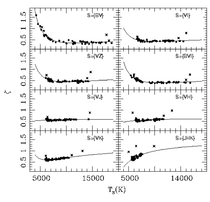
Figure 22: Dilution factors $\zeta$ computed from E96 atmosphere models vs. color temperature derived from eight different filter subsets. The solid lines correspond to a polynomial fit to $\zeta(T_{S})$, from which three deviant models (shown with crosses) are removed.

Figure 22 shows the resulting $\zeta_{S}$ factors for eight filter combinations. The differences between the new dilution factors and those of E96 are less than 5% and, not surprisingly, we recover the result that $\zeta_{S}$ is primarily determined by temperature. For convenience, therefore, we perform polynomial fits to $\zeta_{S}(T_{S})\approx z(T_{S})$, where

$$z(T_{S})=\sum_{i=0}^{2}a_{S,i}\left\{\frac{10^{4}K}{T_{S}}\right\}^{i}.$$ (C2)

Table 14 gives the resulting coefficients $a_{S,i}$ for the nine filter subsets and in Figure 22 we compare these fits to the individual $\zeta_{S}$ factors. Following E96, we remove the peculiar models s15.5.1, s25.5.1, and h10.30.1 (shown with crosses), as they are not appropriate models for SNe II-P.

Appendix D THE $Z$-BAND PHOTOMETRIC SYSTEM

We define the $Z$-band as the product of the transmission of the $Z$ filter (number 611) and the QE of CCD TEK36 of the NTT/EMMI instrument. The resulting bandpass also includes telluric lines (see Figure 19). We employ this filter function to compute synthetic magnitudes from the tertiary spectrophotometric standards published by Hamuy et al. (1994). However, since these spectra contain telluric lines it is necessary first to remove these features. Then we use equation B1 and an adopted ZP of 32.724 that yields a magnitude of 0.03 for Vega. We choose this ZP so that $(V-Z)$=0 for Vega. The resulting synthetic magnitudes for the tertiary standards are listed in Table 15 and this is the system relative to which we calibrated a photometric sequence around SN 1999em. In Hamuy et al. (1994) we showed that synthetic magnitudes in the $I$ band had typical uncertainties of 0.018 mag. Therefore, we believe that the $Z$ magnitudes in Table 15 have errors of 0.02 mag.

Table 1: $UBVRIZ$ Photometry of SN 1999em

JD	$U$	$B$	$V$	$R$	$I$	$Z$	Telescope
-2451000
481.76	$\cdots$	$\cdots$	$\cdots$	$\cdots$	$\cdots$	13.703(015)	CTIO 0.9-m
483.72	$\cdots$	$\cdots$	$\cdots$	$\cdots$	$\cdots$	13.607(015)	CTIO 0.9-m
484.76	$\cdots$	$\cdots$	$\cdots$	$\cdots$	$\cdots$	13.570(015)	CTIO 0.9-m
485.79	$\cdots$	$\cdots$	$\cdots$	$\cdots$	$\cdots$	13.542(015)	CTIO 0.9-m
486.80	$\cdots$	$\cdots$	$\cdots$	$\cdots$	$\cdots$	13.549(015)	CTIO 0.9-m
487.76	$\cdots$	$\cdots$	$\cdots$	$\cdots$	$\cdots$	13.512(015)	CTIO 0.9-m
488.80	$\cdots$	$\cdots$	$\cdots$	$\cdots$	$\cdots$	13.514(015)	CTIO 0.9-m
489.81	$\cdots$	$\cdots$	$\cdots$	$\cdots$	$\cdots$	13.489(015)	CTIO 0.9-m
498.78	14.420(017)	14.357(015)	13.869(015)	13.600(015)	13.483(015)	$\cdots$	CTIO 1.5-m
499.81	14.522(017)	14.414(015)	13.894(015)	13.599(015)	13.482(015)	$\cdots$	CTIO 1.5-m
501.75	$\cdots$	$\cdots$	$\cdots$	$\cdots$	$\cdots$	13.296(015)	CTIO 0.9-m
506.77	$\cdots$	$\cdots$	$\cdots$	$\cdots$	$\cdots$	13.265(015)	CTIO 0.9-m
508.82	$\cdots$	$\cdots$	$\cdots$	$\cdots$	$\cdots$	13.241(015)	CTIO 0.9-m
509.86	$\cdots$	$\cdots$	$\cdots$	$\cdots$	$\cdots$	13.234(015)	CTIO 0.9-m
511.85	$\cdots$	14.833(015)	13.968(015)	13.633(015)	13.414(015)	$\cdots$	SO 2.3-m
522.70	16.043(015)	15.142(015)	14.016(015)	13.618(015)	13.351(015)	$\cdots$	SO 1.5-m
531.76	$\cdots$	15.185(015)	14.011(015)	13.577(015)	13.284(015)	$\cdots$	SO 2.3-m
538.56	$\cdots$	$\cdots$	$\cdots$	$\cdots$	$\cdots$	13.090(015)	CTIO 0.9-m
540.55	$\cdots$	$\cdots$	$\cdots$	$\cdots$	$\cdots$	13.102(015)	CTIO 0.9-m
546.55	$\cdots$	$\cdots$	$\cdots$	$\cdots$	$\cdots$	13.112(015)	CTIO 0.9-m
550.55	$\cdots$	$\cdots$	$\cdots$	$\cdots$	$\cdots$	13.108(015)	CTIO 0.9-m
578.63	$\cdots$	16.060(015)	14.409(015)	13.828(015)	13.492(015)	$\cdots$	SO 1.5-m
607.64	$\cdots$	18.388(040)	16.467(015)	15.541(015)	14.956(015)	$\cdots$	SO 1.5-m
636.04	21.300(400)	18.370(030)	16.658(015)	15.721(015)	15.239(015)	14.924(015)	ESO NTT
665.97	$\cdots$	18.600(035)	16.968(015)	15.999(015)	15.503(025)	$\cdots$	ESO NTT

Table 2: Journal of the Spectroscopic Observations

UT Date	Julian Date	Observatory	Telescope	Wavelength	Dispersion	Weather	Observer(s)
	-2451000			($\mu$)	(Å/pix)
1999 Oct 30	481.79	Tololo	1.5-m	0.33-0.97	5.7	$\cdots$	Smith
1999 Nov 2	484.64	Paranal	VLT/Antu	0.98-2.50	2.9-7.1	Clear	Hamuy,Lidman,Petr
1999 Nov 3	485.67	La Silla	NTT	0.33-1.01	2.7-3.5	Clear?	Maza
1999 Nov 9	491.67	La Silla	NTT	0.33-1.00	2.7-3.5	Clear	Hamuy,Brillant
1999 Nov 14	496.67	La Silla	NTT	0.33-1.01	2.7-3.5	Clear	Hamuy,Doublier
1999 Nov 18	500.64	Paranal	VLT/Antu	0.98-2.54	2.9-7.1	Clear	Service Observing
1999 Nov 19	501.66	La Silla	NTT	0.33-1.01	2.7-3.5	Clear	Hamuy,Doublier
1999 Nov 28	510.63	Paranal	VLT/Antu	0.98-2.53	2.9-7.1	Clear	Hamuy,Lidman,Chadid
1999 Dec 16	528.76	Steward	2.3-m	0.49-0.93	3.6	Clear	Corbally,Omizzolo
1999 Dec 31	543.76	Steward	2.3-m	0.33-0.71	3.6	$\cdots$	Burstein,Li

Table 3: Optical Line Identifications and Observed Wavelengths of Absorption Features of SN 1999em

Identif.	$\lambda_{rest}$	Oct 30	Nov 3	Nov 9	Nov 14	Nov 19	Dec 16	Dec 31
		481.79	485.67	491.67	496.67	501.66	528.76	543.76
$\cdots$	$\cdots$	$\cdots$	$\cdots$	3671	3671	3675	$\cdots$	3683
Ca II K	3934	$\cdots$	$\cdots$	3846	3847	3852	$\cdots$	3868
Ca II H	3968	$\cdots$	$\cdots$	3846	3847	3852	$\cdots$	3868
H$\delta$	4102	$\cdots$	3996	4016	4021	4029	$\cdots$	4025
$\cdots$	$\cdots$	$\cdots$	$\cdots$	$\cdots$	4095	4107	$\cdots$	$\cdots$
Sr II + Ca I + Fe II	4225	$\cdots$	$\cdots$	$\cdots$	$\cdots$	4169	$\cdots$	4178
H$\gamma$	4340	4214	4224	4234	4240	4246	$\cdots$	4260
Ti II	4395	$\cdots$	$\cdots$	$\cdots$	$\cdots$	4318	$\cdots$	4342
$\cdots$	$\cdots$	$\cdots$	$\cdots$	$\cdots$	$\cdots$	$\cdots$	$\cdots$	4412
Ba II + Ti II	4552	$\cdots$	4370	4425	4458	4473	$\cdots$	4500
N II	4623	$\cdots$	$\cdots$	$\cdots$	$\cdots$	$\cdots$	$\cdots$	4588
$\cdots$	$\cdots$	$\cdots$	$\cdots$	$\cdots$	$\cdots$	$\cdots$	$\cdots$	4626
$\cdots$	$\cdots$	$\cdots$	$\cdots$	$\cdots$	$\cdots$	$\cdots$	$\cdots$	4693
H$\beta$	4861	4694	4721	4735	4746	4761	$\cdots$	4763
$\cdots$	$\cdots$	$\cdots$	$\cdots$	$\cdots$	$\cdots$	4836	$\cdots$	4817
Fe II + Ba II	4929	$\cdots$	$\cdots$	$\cdots$	$\cdots$	$\cdots$	$\cdots$	4874
Fe II	5018	$\cdots$	$\cdots$	4911	4920	4934	4965	4969
Fe II + Mg I +Ti II	5185	$\cdots$	$\cdots$	5047	5065	5081	5113	5117
$\cdots$	$\cdots$	$\cdots$	$\cdots$	$\cdots$	$\cdots$	$\cdots$	5178	5182
Fe I	5270	$\cdots$	$\cdots$	5178	5208	5229	5221	5229
$\cdots$	$\cdots$	$\cdots$	$\cdots$	$\cdots$	$\cdots$	$\cdots$	5263	5270
$\cdots$	$\cdots$	$\cdots$	$\cdots$	$\cdots$	$\cdots$	$\cdots$	5373	5376
Sc II + Fe II	5531	$\cdots$	$\cdots$	$\cdots$	$\cdots$	5437	5475	5481
Na I + Sc II	5685	$\cdots$	$\cdots$	$\cdots$	$\cdots$	$\cdots$	5607	5612
He I	5876	5665	5718	$\cdots$	$\cdots$	$\cdots$	$\cdots$	$\cdots$
Na I	5893	$\cdots$	$\cdots$	$\cdots$	$\cdots$	5789	5829	5831
Fe II + Ba II	6146	$\cdots$	$\cdots$	$\cdots$	$\cdots$	6042	6086	6093
Fe II + Sc II	6244	$\cdots$	$\cdots$	$\cdots$	$\cdots$	6144	6184	6194
Si II	6355	$\cdots$	$\cdots$	$\cdots$	$\cdots$	$\cdots$	6316	6319
H$\alpha$	6563	6292	6337	6362	6379	6392	6455	$\cdots$
Ca II	8498+8542+8662	$\cdots$	$\cdots$	$\cdots$	$\cdots$	8344	8380	$\cdots$

Note. — All wavelengths are measured in Å in the SN rest frame.

Table 4: IR Line Identifications and Observed Wavelengths of Absorption Features of SN 1999em

Identif.	$\lambda_{rest}$	Nov 2	Nov 18	Nov 28
		484.64	500.64	510.63
P$\delta$	10049	$\cdots$	9901	9909
$\cdots$	$\cdots$	$\cdots$	$\cdots$	10180
$\cdots$	$\cdots$	$\cdots$	10418	10418
$\cdots$	$\cdots$	$\cdots$	$\cdots$	10549
He I	10830	10503	$\cdots$	$\cdots$
P$\gamma$	10938	$\cdots$	10741	10788
P$\beta$	12818	12473	12573	12627
B$\theta$	16412	$\cdots$	$\cdots$	16219
B$\eta$	16811	$\cdots$	16566	16612
B$\zeta$	17367	$\cdots$	17108	17150
B$\epsilon$	18179	$\cdots$	17884	17949
P$\alpha$	18751	$\cdots$	$\cdots$	$\cdots$
B$\delta$	19445	$\cdots$	$\cdots$	19210
B$\gamma$	21656	$\cdots$	21289	21368

Note. — All wavelengths are measured in Å in the SN rest frame.

Table 5: Expansion Velocities for SN 1999em from Cross-Correlation

JD	model	$v_{model}$	$v_{CC}$	$v_{model}-v_{SN}$	$v_{SN}$
-2451000		(km s-1)	(km s-1)	(km s-1)	(km s-1)
481.79	p12.10.5	10992	-614	-728	11720
481.79	p12.10.6	11002	-591	-700	11702
481.79	p12.10.9	11001	-744	-881	11882
481.79	s15.12.4	11403	720	847	10556
481.79	s15.12.5	11251	401	470	10781
484.64	p9.10.1	11594	-206	-287	11881
484.64	p9.10.2	11564	274	375	11189
484.64	p9.10.3	11329	477	655	10674
484.64	p9.10.4	11375	-366	-508	11883
484.64	p12.10.3	8481	-1656	-2288	10769
484.64	p12.10.5	10992	-84	-119	11111
484.64	p12.10.8	10984	575	791	10194
484.64	p12.10.11	10619	714	982	9637
484.64	s15.12.1	11494	1329	1831	9663
484.64	s15.12.2	11256	262	359	10897
484.64	s15.12.4	11403	647	890	10513
484.64	s15.12.5	11251	253	346	10905
485.67	p9.10.1	11594	467	548	11046
485.67	p9.10.2	11564	454	533	11031
485.67	p9.10.3	11329	240	280	11049
485.67	p9.10.4	11375	114	132	11243
485.67	p12.10.1	11141	875	1030	10112
485.67	p12.10.2	11103	952	1120	9983
485.67	p12.10.3	8481	-538	-638	9119
485.67	p12.10.8	10984	574	674	10310
485.67	p12.10.10	10922	686	806	10116
485.67	p12.10.11	10619	645	758	9861
485.67	s15.12.1	11494	2218	2614	8880
485.67	s15.12.2	11256	1866	2199	9057
485.67	s15.12.3	11461	2344	2763	8698
485.67	s15.19.6	9590	-190	-227	9817
491.67	p6.10.1	12653	2059	2427	10226
491.67	p12.10.4	11058	2061	2429	8629
491.67	s15.19.1	10804	2451	2889	7915
491.67	s15.19.2	10644	2382	2808	7836
491.67	s15.19.3	10276	2449	2887	7389
491.67	s15.19.4	10275	2479	2922	7353
491.67	s15.20.1	10520	2532	2985	7535
491.67	s15.28.2	9654	1665	1962	7692
491.67	s15.28.4	8990	559	657	8333
491.67	s25.30.1	5816	477	560	5256
496.67	s15.28.1	9438	2484	2928	6510
496.67	s15.28.2	9654	2471	2913	6741
496.67	s15.28.3	10230	2599	3064	7166
496.67	s15.28.5	9170	1436	1691	7479
496.67	s25.30.1	5816	384	450	5366
500.64	p6.40.2	8624	1866	2572	6052
500.64	p6.60.1	5409	236	323	5086
500.64	p6.60.2	5170	95	128	5042
500.64	p6.60.3	5384	101	136	5248
500.64	p6.60.4	5263	158	215	5048
500.64	p6.60.6	5409	253	346	5063
500.64	s15.40.1	7040	1834	2528	4512
500.64	s15.43.2	7241	1563	2154	5087
500.64	s15.46.1	6453	1220	1681	4772
500.64	s15.46.2	6707	1404	1935	4772
500.64	s15.60.4	5215	318	436	4779
500.64	s25.60.1	4667	310	425	4242
501.66	p6.40.2	8624	2398	2827	5797
501.66	p6.60.1	5409	200	233	5176
501.66	p6.60.2	5170	154	179	4991
501.66	p6.60.3	5384	464	545	4839
501.66	p6.60.4	5263	293	343	4920
501.66	p6.60.6	5409	185	215	5194
501.66	p9.60.1	4709	-13	-18	4727
501.66	s15.40.1	7040	1830	2156	4884
501.66	s15.43.2	7241	1608	1894	5347
501.66	s15.43.3	6300	1707	2011	4289
501.66	s15.46.1	6453	1169	1376	5077
501.66	s15.46.2	6707	1745	2056	4651
501.66	s15.60.4	5215	709	834	4381
501.66	s25.60.1	4667	-607	-719	5386
510.63	p6.40.3	7686	1860	2564	5122
510.63	p6.60.1	5409	475	653	4757
510.63	p6.60.2	5170	504	693	4477
510.63	p6.60.4	5263	575	791	4473
510.63	p6.60.5	4872	573	788	4084
510.63	p6.60.6	5409	492	676	4733
510.63	p9.60.1	4709	336	461	4248
510.63	p12.60.1	4418	-106	-149	4567
510.63	s15.40.1	7040	2223	3065	3975
510.63	s15.43.1	6476	1494	2059	4417
510.63	s15.43.2	7241	1908	2630	4611
510.63	s15.43.3	6300	1709	2355	3945
510.63	s15.46.1	6453	1621	2234	4219
510.63	s15.46.2	6707	1799	2480	4227
510.63	s15.60.1	3438	-463	-642	4080
510.63	s15.60.2	5794	863	1188	4606
510.63	s15.60.3	3452	-261	-363	3815
510.63	s15.60.4	5215	698	960	4255
510.63	s25.60.1	4667	750	1032	3635
510.63	h10.30.1	3864	-668	-925	4789
510.63	h10.60.1	2786	-453	-628	3414
528.76	p6.40.1	7340	3290	3879	3461
528.76	p6.40.3	7686	3481	4105	3581
528.76	p6.60.5	4872	1595	1879	2993
528.76	s15.60.1	3438	1003	1181	2257
528.76	s15.60.3	3452	837	985	2467
528.76	h10.30.1	3864	711	836	3028
528.76	h10.60.1	2786	140	162	2624
543.76	p6.40.1	7340	3861	4553	2787
543.76	s15.60.1	3439	1430	1684	1755
543.76	s15.60.3	3452	1297	1527	1925
543.76	h10.30.1	3864	1472	1734	2130

Table 6: Expansion Velocities for SN 1999em

JD	$v_{lines}$	$v_{Fe}$	$v_{Sc}$	$v_{CC}$
-2451000	(km s-1)	(km s-1)	(km s-1)	(km s-1)
481.79	$\cdots$	$\cdots$	$\cdots$	11328(611)
484.64	$\cdots$	$\cdots$	$\cdots$	10776(721)
485.67	8067	$\cdots$	$\cdots$	10023(859)
491.67	6997(1451)	6739(483)	$\cdots$	7817(1238)
496.67	5631(1473)	5947(125)	$\cdots$	6652(811)
500.64	$\cdots$	$\cdots$	$\cdots$	4975(442)
501.66	4808(1004)	5065(60)	4831	4976(402)
510.63	$\cdots$	$\cdots$	$\cdots$	4307(415)
528.76	3132(702)	3209(58)	2736(46)	2916(496)
543.76	2972(661)	2973(63)	2441(3)	2149(452)

Table 7: EPM Quantities Derived for SN 1999em from Subsets {BV} and {VI}

JD-	$v_{ph}$	$T_{BV}$	$\theta\zeta_{BV}$	$\zeta_{BV}$	($\theta$/$v$)BV	$T_{VI}$	$\theta\zeta_{VI}$	$\zeta_{VI}$	($\theta$/$v$)VI
2451000	(km s-1)	(K)	(1011cm Mpc-1)		(100 s Mpc-1)	(K)	(1011cm Mpc-1)		(100 s Mpc-1)
481.76	11763	19490(1471)	220(16)	0.431	433(39)	13392(589)	323(15)	0.453	606(41)
481.80	11741	18387(1292)	234(17)	0.420	475(41)	12683(487)	347(14)	0.448	661(43)
483.72	10752	16362(990)	270(18)	0.400	627(52)	12966(512)	348(15)	0.450	719(47)
483.78	10722	16087(1613)	278(30)	0.397	652(77)	14501(1685)	310(38)	0.461	627(84)
484.76	10255	15122(830)	297(19)	0.388	747(60)	12870(504)	356(15)	0.449	773(50)
485.79	9788	14524(759)	305(19)	0.383	813(65)	12683(487)	356(15)	0.448	811(53)
486.80	9354	14278(730)	309(19)	0.381	869(69)	11717(408)	391(15)	0.441	946(60)
487.76	8964	13878(685)	316(19)	0.377	934(73)	11086(359)	415(16)	0.438	1057(66)
488.80	8562	13064(598)	338(20)	0.372	1060(82)	10649(328)	437(16)	0.437	1168(73)
489.81	8194	12709(1119)	347(38)	0.370	1146(139)	10320(709)	454(41)	0.436	1271(132)
490.79	7857	12059(728)	367(29)	0.367	1271(118)	9766(270)	486(17)	0.436	1421(87)
492.79	7224	10467(366)	449(24)	0.371	1675(122)	9804(272)	492(18)	0.436	1563(96)
493.74	6949	9869(322)	490(26)	0.378	1867(135)	9791(271)	496(18)	0.436	1638(101)
495.67	6437	8659(295)	596(35)	0.410	2258(174)	9640(360)	506(26)	0.436	1802(129)
495.74	6419	8086(209)	676(33)	0.438	2401(168)	9882(277)	494(18)	0.436	1766(109)
498.65	5758	7096(182)	849(45)	0.521	2833(207)	9531(291)	517(21)	0.436	2059(134)
498.68	5752	7081(159)	844(40)	0.522	2810(195)	9251(239)	535(19)	0.437	2128(129)
498.78	5731	7385(173)	773(37)	0.491	2749(191)	9229(237)	533(18)	0.437	2126(129)
499.81	5527	7133(161)	816(39)	0.516	2859(198)	8948(221)	552(19)	0.439	2276(138)
500.70	5362	6906(233)	858(60)	0.543	2944(254)	8937(341)	547(31)	0.439	2321(174)
501.71	5187	6388(128)	1023(48)	0.622	3173(218)	8906(219)	560(19)	0.439	2456(149)
501.75	5180	6537(135)	967(46)	0.596	3131(216)	8855(216)	560(19)	0.440	2459(149)
502.67	5031	6486(210)	982(70)	0.605	3229(281)	8449(391)	604(44)	0.444	2702(239)
504.67	4738	5917(183)	1197(87)	0.720	3507(310)	8676(259)	578(26)	0.442	2764(185)
504.74	4728	6093(151)	1109(65)	0.680	3452(265)	8252(185)	621(20)	0.447	2937(176)
505.72	4600	5687(102)	1294(61)	0.781	3601(247)	8296(187)	614(20)	0.446	2991(179)
506.77	4472	5815(106)	1219(57)	0.746	3652(250)	8065(176)	638(21)	0.450	3169(189)
507.80	4356	5488(138)	1399(90)	0.843	3811(311)	8090(177)	636(21)	0.450	3246(194)
508.82	4249	5579(98)	1338(63)	0.814	3870(265)	7983(172)	648(21)	0.452	3371(201)
509.86	4148	5323(95)	1498(74)	0.901	4009(282)	7983(172)	647(21)	0.452	3448(205)
510.75	4068	5252(87)	1556(73)	0.928	4123(282)	7779(162)	680(22)	0.457	3657(217)
511.85	3976	5224(86)	1562(73)	0.939	4185(287)	7696(158)	686(22)	0.459	3760(223)
513.72	3835	5021(80)	1739(81)	1.026	4417(303)	7522(161)	718(25)	0.464	4038(245)
516.71	3645	4770(75)	1985(96)	1.155	4718(327)	7369(144)	742(23)	0.469	4342(256)
519.72	3485	4571(67)	2243(105)	1.276	5043(346)	7263(139)	764(24)	0.473	4635(273)
522.59	3353	4449(63)	2433(114)	1.361	5333(366)	7191(136)	780(24)	0.475	4891(288)
522.70	3348	4338(60)	2555(120)	1.445	5281(363)	6956(126)	809(25)	0.486	4977(292)
527.63	3139	4360(256)	2562(461)	1.427	5720(1067)	7289(349)	754(64)	0.472	5095(501)
528.59	3098	4307(82)	2650(163)	1.470	5819(461)	6799(151)	859(35)	0.494	5617(361)
531.76	2956	4205(57)	2816(133)	1.556	6122(421)	6607(113)	899(27)	0.505	6023(352)
538.56	2584	3981(53)	3328(162)	1.776	7250(506)	6507(129)	920(34)	0.511	6962(433)
538.60	2582	3894(85)	3618(286)	1.875	7475(699)	6618(196)	897(49)	0.504	6895(513)
540.55	2451	3941(71)	3394(216)	1.821	7605(615)	6523(160)	902(43)	0.510	7216(497)
546.55	2176	3792(47)	3851(183)	1.999	8850(611)	6332(103)	956(29)	0.524	8392(489)
546.61	2176	3823(54)	3781(200)	1.960	8865(646)	6436(107)	933(28)	0.516	8311(485)
547.60	2172	3768(53)	3977(211)	2.031	9018(658)	6426(106)	937(28)	0.517	8347(487)
550.55	2159	3733(75)	4058(299)	2.077	9051(806)	6337(161)	953(48)	0.523	8437(600)
551.61	2154	3752(46)	3970(189)	2.051	8988(621)	6260(100)	974(29)	0.529	8547(497)
551.66	2154	3693(45)	4258(203)	2.133	9271(641)	6308(102)	972(29)	0.525	8589(500)

Table 8: EPM Quantities Derived for SN 1999em from Subsets {BVI} and {VZ}

JD-	$v_{ph}$	$T_{BVI}$	$\theta\zeta_{BVI}$	$\zeta_{BVI}$	($\theta$/$v$)BVI	$T_{VZ}$	$\theta\zeta_{VZ}$	$\zeta_{VZ}$	($\theta$/$v$)VZ
2451000	(km s-1)	(K)	(1011cm Mpc-1)		(100 s Mpc-1)	(K)	(1011cm Mpc-1)		(100 s Mpc-1)
481.76	11763	15674(448)	278(8)	0.443	533(31)	12827(409)	339(11)	0.475	607(36)
481.80	11741	14707(364)	301(8)	0.435	589(33)	$\cdots$	$\cdots$	$\cdots$	$\cdots$
483.72	10752	14295(341)	316(8)	0.431	682(39)	12526(388)	362(12)	0.472	713(43)
483.78	10722	15434(1071)	291(22)	0.441	615(55)	$\cdots$	$\cdots$	$\cdots$	$\cdots$
484.76	10255	13794(315)	332(9)	0.427	759(43)	12454(382)	370(12)	0.472	766(46)
485.79	9788	13451(297)	335(9)	0.424	807(45)	11335(309)	409(13)	0.462	904(53)
486.80	9354	12741(263)	358(9)	0.419	913(51)	11335(309)	407(13)	0.462	943(55)
487.76	8964	12181(238)	375(9)	0.416	1007(56)	10543(262)	444(13)	0.457	1084(63)
488.80	8562	11608(213)	397(9)	0.413	1122(62)	10469(258)	447(13)	0.457	1142(66)
489.81	8194	11386(545)	402(25)	0.412	1190(96)	10073(297)	470(16)	0.456	1257(76)
490.79	7857	10378(219)	453(12)	0.412	1398(80)	$\cdots$	$\cdots$	$\cdots$	$\cdots$
492.79	7224	10091(156)	475(10)	0.413	1593(87)	$\cdots$	$\cdots$	$\cdots$	$\cdots$
493.74	6949	9826(147)	494(11)	0.415	1714(93)	$\cdots$	$\cdots$	$\cdots$	$\cdots$
495.67	6437	9135(192)	543(18)	0.422	2001(120)	$\cdots$	$\cdots$	$\cdots$	$\cdots$
495.74	6419	8981(120)	556(12)	0.424	2041(111)	$\cdots$	$\cdots$	$\cdots$	$\cdots$
498.65	5758	8267(127)	626(16)	0.441	2463(139)	$\cdots$	$\cdots$	$\cdots$	$\cdots$
498.68	5752	8132(97)	635(13)	0.446	2476(134)	$\cdots$	$\cdots$	$\cdots$	$\cdots$
498.78	5731	8299(101)	612(12)	0.440	2427(131)	$\cdots$	$\cdots$	$\cdots$	$\cdots$
499.81	5527	8033(94)	638(13)	0.449	2572(139)	$\cdots$	$\cdots$	$\cdots$	$\cdots$
500.70	5362	7919(171)	652(24)	0.453	2680(167)	$\cdots$	$\cdots$	$\cdots$	$\cdots$
501.71	5187	7572(83)	700(14)	0.469	2876(155)	$\cdots$	$\cdots$	$\cdots$	$\cdots$
501.75	5180	7644(85)	686(14)	0.466	2843(153)	8088(144)	650(17)	0.473	2654(149)
502.67	5031	7288(173)	766(35)	0.485	3136(212)	$\cdots$	$\cdots$	$\cdots$	$\cdots$
504.67	4738	7527(141)	713(23)	0.472	3191(191)	$\cdots$	$\cdots$	$\cdots$	$\cdots$
504.74	4728	7340(95)	734(17)	0.482	3222(177)	$\cdots$	$\cdots$	$\cdots$	$\cdots$
505.72	4600	6897(68)	805(16)	0.513	3411(183)	$\cdots$	$\cdots$	$\cdots$	$\cdots$
506.77	4472	6889(68)	807(16)	0.514	3510(188)	7587(125)	710(18)	0.487	3259(183)
507.80	4356	7063(94)	777(18)	0.501	3562(197)	$\cdots$	$\cdots$	$\cdots$	$\cdots$
508.82	4249	6710(64)	841(16)	0.530	3738(200)	7409(119)	739(18)	0.495	3519(197)
509.86	4148	6609(66)	861(17)	0.540	3848(207)	7354(117)	749(19)	0.497	3632(203)
510.75	4068	6426(58)	914(17)	0.559	4018(215)	$\cdots$	$\cdots$	$\cdots$	$\cdots$
511.85	3976	6376(57)	920(17)	0.565	4098(219)	$\cdots$	$\cdots$	$\cdots$	$\cdots$
513.72	3835	6130(57)	1004(21)	0.597	4386(237)	$\cdots$	$\cdots$	$\cdots$	$\cdots$
516.71	3645	5992(52)	1040(20)	0.617	4626(248)	$\cdots$	$\cdots$	$\cdots$	$\cdots$
519.72	3485	5791(47)	1114(21)	0.650	4915(262)	$\cdots$	$\cdots$	$\cdots$	$\cdots$
522.59	3353	5684(45)	1160(22)	0.670	5161(275)	$\cdots$	$\cdots$	$\cdots$	$\cdots$
522.70	3348	5528(43)	1205(22)	0.702	5127(273)	$\cdots$	$\cdots$	$\cdots$	$\cdots$
527.63	3139	6360(221)	961(68)	0.567	5401(468)	$\cdots$	$\cdots$	$\cdots$	$\cdots$
528.59	3098	5567(67)	1245(35)	0.694	5793(333)	$\cdots$	$\cdots$	$\cdots$	$\cdots$
531.76	2956	5316(39)	1329(25)	0.751	5984(319)	$\cdots$	$\cdots$	$\cdots$	$\cdots$
538.56	2584	5030(42)	1519(35)	0.832	7064(388)	6347(85)	969(23)	0.565	6632(367)
538.60	2582	5134(73)	1468(54)	0.801	7101(441)	$\cdots$	$\cdots$	$\cdots$	$\cdots$
540.55	2451	5120(64)	1475(48)	0.805	7479(446)	6272(82)	979(23)	0.573	6977(386)
546.55	2176	4941(34)	1530(28)	0.861	8168(435)	6280(83)	973(23)	0.572	7819(432)
546.61	2176	5123(41)	1424(28)	0.804	8139(438)	$\cdots$	$\cdots$	$\cdots$	$\cdots$
547.60	2172	5083(40)	1448(29)	0.816	8176(440)	$\cdots$	$\cdots$	$\cdots$	$\cdots$
550.55	2159	5002(69)	1559(56)	0.841	8589(530)	6249(84)	982(24)	0.575	7907(439)
551.61	2154	4890(33)	1563(29)	0.878	8262(440)	$\cdots$	$\cdots$	$\cdots$	$\cdots$
551.66	2154	4864(33)	1597(29)	0.887	8359(445)	$\cdots$	$\cdots$	$\cdots$	$\cdots$

Table 9: EPM Quantities Derived for SN 1999em from Subsets {VJ} and {VH}

JD-	$v_{ph}$	$T_{VJ}$	$\theta\zeta_{VJ}$	$\zeta_{VJ}$	($\theta$/$v$)VJ	$T_{VH}$	$\theta\zeta_{VH}$	$\zeta_{VH}$	($\theta$/$v$)VH
2451000	(km s-1)	(K)	(1011cm Mpc-1)		(100 s Mpc-1)	(K)	(1011cm Mpc-1)		(100 s Mpc-1)
481.80	11741	13207(318)	331(8)	0.586	481(27)	11318(192)	400(7)	0.590	578(31)
482.69	11271	10963(348)	421(17)	0.581	643(41)	10338(178)	456(9)	0.583	693(37)
483.76	10732	10993(210)	427(9)	0.581	685(37)	10541(163)	452(8)	0.585	720(38)
483.78	10722	12596(342)	364(10)	0.585	581(33)	9923(207)	498(13)	0.581	800(45)
484.76	10255	11310(224)	418(9)	0.582	700(38)	10706(169)	449(8)	0.586	748(40)
485.73	9815	10714(488)	440(26)	0.580	773(60)	10279(284)	466(17)	0.583	815(50)
486.77	9367	10218(178)	469(9)	0.579	864(47)	9909(142)	489(8)	0.580	900(47)
487.75	8968	10102(173)	471(9)	0.578	909(49)	9836(140)	490(8)	0.580	942(50)
488.76	8577	9645(156)	502(10)	0.577	1015(54)	9525(130)	511(8)	0.577	1033(54)
489.81	8194	9464(188)	514(11)	0.576	1089(59)	9304(155)	527(9)	0.576	1118(59)
495.74	6419	9211(141)	548(10)	0.575	1483(79)	9206(120)	548(9)	0.575	1486(78)
498.68	5752	9305(240)	531(19)	0.576	1602(99)	9252(245)	535(21)	0.575	1618(102)
501.71	5187	7668(93)	719(13)	0.568	2438(129)	8324(96)	624(9)	0.566	2125(111)
504.74	4728	8530(118)	588(11)	0.572	2172(116)	7983(87)	657(10)	0.562	2469(129)
505.72	4600	7943(101)	661(12)	0.570	2524(134)	7646(79)	707(10)	0.558	2752(143)
507.80	4356	7775(96)	681(12)	0.569	2751(146)	7834(129)	673(18)	0.561	2754(156)
510.75	4068	7744(95)	685(12)	0.569	2962(157)	7653(79)	699(10)	0.558	3079(160)
513.72	3835	7418(89)	737(13)	0.567	3389(180)	7475(119)	727(19)	0.556	3406(193)
516.71	3645	6643(68)	906(15)	0.562	4428(233)	6953(64)	828(12)	0.549	4140(215)
519.72	3485	6980(76)	823(14)	0.564	4189(221)	7067(71)	804(13)	0.550	4190(219)
522.59	3353	7056(77)	808(14)	0.565	4271(225)	6885(63)	848(12)	0.548	4616(239)
527.63	3139	6804(95)	861(17)	0.563	4874(261)	6809(82)	860(13)	0.547	5011(262)
528.59	3098	6793(71)	860(14)	0.563	4935(260)	6740(60)	874(12)	0.545	5172(268)
538.60	2582	6549(80)	917(16)	0.561	6329(336)	6557(68)	914(13)	0.542	6529(340)
546.61	2176	6375(62)	952(15)	0.560	7818(411)	6352(52)	959(13)	0.539	8182(424)
547.60	2172	6286(60)	981(16)	0.559	8084(425)	6399(53)	945(13)	0.540	8063(417)
551.66	2154	6491(64)	916(15)	0.561	7585(399)	6463(55)	924(12)	0.541	7933(411)

Table 10: EPM Quantities Derived for SN 1999em from Subsets {VK} and {JHK}

JD-	$v_{ph}$	$T_{VK}$	$\theta\zeta_{VK}$	$\zeta_{VK}$	($\theta$/$v$)VK	$T_{JHK}$	$\theta\zeta_{JHK}$	$\zeta_{JHK}$	($\theta$/$v$)JHK
2451000	(km s-1)	(K)	(1011cm Mpc-1)		(100 s Mpc-1)	(K)	(1011cm Mpc-1)		(100 s Mpc-1)
481.80	11741	9944(130)	477(7)	0.698	583(30)	5640(164)	727(22)	0.628	987(57)
482.69	11271	9165(209)	543(18)	0.673	716(43)	6337(484)	693(50)	0.721	852(75)
483.76	10732	9451(116)	528(8)	0.682	722(38)	6574(232)	681(22)	0.749	848(51)
483.78	10722	8970(166)	579(15)	0.667	810(45)	4732(167)	970(41)	0.465	1947(128)
484.76	10255	9607(142)	523(10)	0.687	743(40)	6736(278)	666(26)	0.766	848(54)
485.73	9815	9642(405)	511(31)	0.688	757(59)	7532(1186)	601(83)	0.842	728(107)
486.77	9367	9079(106)	557(8)	0.670	888(46)	6716(244)	689(23)	0.764	962(58)
487.75	8968	9014(105)	558(8)	0.668	932(48)	6731(245)	684(23)	0.766	996(60)
488.76	8577	8850(107)	572(9)	0.663	1006(53)	7118(294)	662(25)	0.805	959(60)
489.81	8194	8563(117)	601(9)	0.654	1121(58)	6592(234)	721(24)	0.751	1172(70)
495.74	6419	9094(130)	559(10)	0.670	1298(69)	8814(520)	569(28)	0.934	949(66)
498.68	5752	8276(147)	639(18)	0.645	1722(98)	6160(435)	789(54)	0.700	1960(166)
501.71	5187	7705(81)	712(11)	0.629	2184(114)	8580(458)	635(28)	0.919	1332(89)
504.74	4728	7520(74)	730(10)	0.624	2472(129)	5447(160)	939(29)	0.598	3323(195)
505.72	4600	7379(81)	754(13)	0.621	2640(140)	6020(220)	880(32)	0.682	2807(174)
507.80	4356	7298(106)	764(19)	0.619	2834(158)	6417(329)	827(43)	0.731	2597(188)
510.75	4068	7388(132)	746(23)	0.621	2951(174)	6825(363)	776(40)	0.776	2461(176)
513.72	3835	7024(87)	816(17)	0.614	3468(189)	6177(286)	890(42)	0.702	3306(228)
516.71	3645	6809(56)	863(11)	0.610	3879(200)	7613(323)	782(29)	0.848	2529(157)
519.72	3485	6495(50)	951(11)	0.607	4495(231)	5356(146)	1093(31)	0.583	5384(311)
522.59	3353	6815(68)	865(14)	0.610	4228(223)	6077(225)	949(35)	0.689	4109(256)
527.63	3139	6439(67)	963(13)	0.607	5056(262)	5555(163)	1069(32)	0.615	5539(324)
528.59	3098	6469(53)	950(13)	0.607	5054(262)	5659(175)	1047(33)	0.631	5360(317)
538.60	2582	6127(54)	1055(13)	0.607	6733(347)	5116(132)	1206(34)	0.541	8636(494)
546.61	2176	6261(64)	989(19)	0.606	7495(401)	6004(235)	1016(40)	0.679	6871(439)
547.60	2172	6240(49)	997(13)	0.606	7570(392)	6207(215)	988(33)	0.706	6451(389)
551.66	2154	6339(48)	962(12)	0.606	7368(379)	5892(181)	1016(31)	0.664	7104(416)

Table 11: Distance and Explosion Time for SN 1999em

Filter	$D$	$t_{0}$
Subsets	(Mpc)	(JD-2451000)
{BV}	6.91$\pm$0.09	478.3$\pm$0.4
{BVI}	7.40$\pm$0.08	477.9$\pm$0.3
{VI}	7.31$\pm$0.10	479.6$\pm$0.4
{VZ}	7.79$\pm$0.10	477.6$\pm$0.3
{VJ}	8.01$\pm$0.29	479.9$\pm$0.8
{VH}	7.82$\pm$0.28	479.8$\pm$0.9
{VK}	8.22$\pm$0.23	479.1$\pm$0.8
{JHK}	8.56$\pm$0.69	477.5$\pm$2.1
All(8)	7.54$\pm$0.08	478.8$\pm$0.5
{BVIJHK}	7.82$\pm$0.15	478.9$\pm$0.5

Table 12: Photometric Zero-points and Synthetic Magnitudes for Vega and the Sun

	$B$	$V$	$R$	$I$	$Z$	$J_{S}$	$H$	$K_{S}$
Zero-point	35.287	34.855	35.060	34.563	32.724	32.230	32.098	32.175
Vega	0.014	0.030	0.042	0.052	0.030	0.00	0.00	0.00
Sun	-26.083	-26.752	-27.120	-27.451	-27.592	-27.918	-28.243	-28.285

Table 13: Fits to $b_{\overline{\lambda}}(T)$

$i$	c${}_{i}(B)$	c${}_{i}(V)$	c${}_{i}(R)$	c${}_{i}(I)$	c${}_{i}(Z)$	c${}_{i}(J_{S})$	c${}_{i}(H)$	c${}_{i}(K_{S})$
0	-45.144	-44.766	-44.597	-44.345	-44.232	-43.913	-43.767	-43.638
1	7.159	6.793	6.628	6.347	6.262	6.022	5.878	5.737
2	-4.301	-4.523	-4.693	-4.732	-4.810	-4.859	-4.914	-4.881
3	2.639	2.695	2.770	2.739	2.778	2.772	2.797	2.757
4	-0.811	-0.809	-0.831	-0.811	-0.825	-0.819	-0.829	-0.813
5	0.098	0.096	0.099	0.096	0.098	0.097	0.098	0.096

Table 14: Fits to $\zeta(T_{S})$

$S$	$a_{0}$	$a_{1}$	$a_{2}$	$\sigma$
$\{BV\}$	0.7557	-0.8997	0.5199	0.048
$\{BVI\}$	0.7336	-0.6942	0.3740	0.027
$\{VI\}$	0.7013	-0.5304	0.2646	0.029
$\{VZ\}$	0.8185	-0.7137	0.3510	0.031
$\{VJ\}$	0.6104	-0.0323	0.0000	0.025
$\{VH\}$	0.6548	-0.0737	0.0000	0.031
$\{VK\}$	1.2865	-0.8571	0.2700	0.051
$\{JHK\}$	1.4787	-0.4799	0.0000	0.046
$\{BVIJHK\}$	1.1551	-0.9790	0.3913	0.024

Table 15: Standard Stars for the $Z$-band

$Star$	$Z$
	$\pm$0.020
LTT 377	10.523
LTT 1020	10.648
EG 21	11.619
LTT 1788	12.369
LTT 2415	11.526
Hiltner 600	10.132
L745-46A	12.670
LTT 3218	11.652
LTT 3864	11.374
LTT 4364	11.181
Feige 56	11.154
LTT 4816	13.792
CD -32	10.041
LTT 6248	10.966
EG 274	11.359
LTT 7379	9.376
LTT 7987	12.437
LTT 9239	11.144
Feige 110	12.249
LTT 9491	14.071

Figure 3: Optical spectroscopic evolution of SN 1999em in AB magnitudes. Julian Day (-2451000) is indicated for each spectrum. Some of the strongest lines are labeled. The $\oplus$ symbols show the main telluric features.

Figure 4: IR spectroscopic evolution of SN 1999em in AB magnitudes. The most prominent features are labeled. Julian Day (-2451000) is indicated for each spectrum.

Figure 5: Combined optical and IR spectra of SN 1999em in AB magnitudes. The IR spectra spectra were obtained one day before the optical observation and the mean Julian Day (-2451000) is indicated next to each spectrum. The flux excess between 7500-10000 Å in the first-epoch spectrum is due to second-order blue light contamination.

Figure 8: Expansion velocity derived from the minimum of spectral metal absorptions in the December 31 spectrum vs. the equivalent width of the absorption.

Figure 10: (a) Optical spectrum taken on JD 2451501.66 (thick line) compared to four models with similar color temperature (thin lines). The horizontal bars show the wavelength ranges (3000-5000, 5700-6700 Å) used in the derivation of relative velocities from the cross correlation technique. (b) Cross correlation function between the observed spectrum and the four models shown above. The two curves with the highest peaks correspond to models p6.60.1 and p6.40.2, both of which match well the observed spectrum. The two lower curves correspond to models s15.43.3 and s15.46.2 which provide a poorer match to the observed spectrum.

Figure 11: Expansion velocity of SN 1999em vs. Julian Day, derived from the cross-correlation technique (solid dots) and the minimum of the spectral absorptions (open dots). The solid and dashed lines represent polynomial fits to the solid and open points, respectively.

Figure 12: EPM distance derived from different filter subsets, as a function of the adopted visual extinction in the host galaxy.

Figure 17: $\theta$/$v$ as a function of time since explosion (JD 2451478.8) for filter subsets $\{BV,VI,VZ,BVI,VJ,VH,VK,JHK\}$. The solid line shows the regression line for $R_{0}$=0, while the dotted line corresponds to the fit obtained with $R_{0}$= 5$\times$10¹³cm (714 R_⊙).

Figure 18: $BVRI$ filters functions of Bessell (1990) meant for use with energy distributions (dotted curves). With solid lines are shown the curves modified for use with photon distributions, to which we added the telluric lines.

Figure 19: $Z$, $J_{S}$, $H$, $K_{S}$ filters functions. Also shown are the QE of TEK36 and NICMOS2 that we employed to construct these functions.

Figure 20: Adopted spectrophotometric calibration for Vega. In the optical ($\lambda$ $\leq$ 10,500 Å) the calibration is from Hayes (1985), and at longer wavelengths we adopted the Kurucz spectrum with parameters $T_{eff}$=9,400 K, log $g$=3.9, [Fe/H]=-0.5, $V_{microturb}$=0.

Figure 21: (a) Relation between color temperature and four different colors in our photometric system. (b) Difference in color temperature between our calibration and that of E96.

References

- Barbon et al. (1979) Barbon, R., Ciatti, F., & Rosino, L. 1979, A&A, 72, 287
- Baron et al. (2000) Baron, E., et al. 2000, ApJ, 545, 444
- Bessell (1983) Bessell, M. S. 1983, PASP, 95, 480
- Bessell (1990) Bessell, M. S. 1990, PASP, 102, 1181
- Bowers et al. (1997) Bowers, E. J. C., Meikle, W. P. S., Geballe, T. R., Walton, N. A., Pinto, P. A., Dhillon, V. S., Howell, S. B., & Harrop-Allin, M. K. 1997, MNRAS, 290, 663
- Cardelli et al. (1989) Cardelli, J. A., Clayton, G. C., & Mathis, J. S. 1989, ApJ, 345, 245
- Cohen et al. (1992) Cohen, M., Walker, R. G., Barlow, M. J., & Deacon, J. R. 1992, AJ, 104, 1650
- Cousins (1971) Cousins, A. W. J. 1971, R. Obs. Ann. No 7
- Cousins (1980) Cousins, A. W. J. 1980, SAAO Circ. 1, 234
- Cousins (1984) Cousins, A. W. J. 1984, SAAO Circ. 8, 69
- Dwek et al. (1983) Dwek, E. et al. 1983, ApJ, 274, 168
- Eastman et al. (1996) Eastman, R. G., Schmidt, B. P., & Kirshner, R. 1996, ApJ, 466, 911 (E96)
- Elias et al. (1981) Elias, J. H., Frogel, J. A., Hackwell, J. A., & Persson, S. E. 1981, ApJ, 251, L13
- Elias et al. (1982) Elias, J. H., Frogel, J. A., Matthews, K., & Neugebauer, G. 1982, AJ, 87, 1029
- Elias et al. (1985) Elias, J. H., Matthews, K., Neugebauer, G., & Persson, S. E. 1985, ApJ, 296, 379
- Elias et al. (1988) Elias, J. H., Gregory, B., Phillips, M. M., Williams, R. E., Graham, J. R., Meikle, W. P. S., Schwartz, R. D., & Wilking, B. 1988, ApJ, 331, L9
- Giovanelli et al. (1997) Giovanelli, R., Haynes, M. P, da Costa, L. N., Freudling, W., Salzer, J. J., & Wegner, G. 1997, ApJ, 477, L1
- Gray & Corbally (1994) Gray, R. O., & Corbally, C. J. 1994, AJ, 107, 742
- Hamuy et al. (1990) Hamuy, M., Suntzeff, N. B., Bravo, J., & Phillips, M. M. 1990, PASP, 102, 888
- Hamuy et al. (1994) Hamuy, M., Suntzeff, N. B., Heathcote, S. R., Walker, A. R., Gigoux, P., & Phillips, M. M. 1994, PASP, 106, 566
- Hayes (1985) Hayes, D. S. 1985, in Calibration of Fundamental Stellar Quantities, ed. D. S. Hayes, L. E. Pasinetti, & A. G. Philip (Dordrecht: Reidel), 225
- Haynes et al. (1998) Haynes, M. P., van Zee, L., Hogg, D. E., Roberts, M. S., & Maddalena, R. J., 1998, AJ, 115, 62
- Jeffery & Branch (1990) Jeffery, D. J., & Branch, D. 1990, in Jerusalem Winter School for Theoretical Physics. Supernovae, Volume 6, ed. J. C. Wheeler, T. Piran, & S. Weinberg (World Scientific Publishing Co., Singapore; Teaneck, N.J.), 149
- Jha et al. (1999) Jha, S., Challis, P., Garnavich, P., & Kirshner, R. 1999, IAUC 7296
- Johnson et al. (1966) Johnson, H. L., Iriarte, B., Mitchell, R. I., & Wisniewskj, W. Z. 1966, Comm. Lunar Plan. Lab., 4, 99
- Kirshner & Kwan (1974) Kirshner, R. P., & Kwan, J. 1974, ApJ, 193, 27
- Kurucz (1995) Kurucz, H. L. 1995, in ASP Conf. Ser. 81, Laboratory and Astronomical High-Resolution Spectra, ed. A. J. Sauval, R. Blomme, & N. Grevesse (San Francisco:ASP), 17
- Leonard et al. (2000) Leonard, D. C., Filippenko, A. V., Ardila, D. R., & Brotherton, M. S. 2000, ApJ, submitted (astro-ph/0009285)
- Li (1999) Li, W. D. 1999, IAUC 7294
- Livingston & Wallace (1991) Livingston, W., & Wallace, L. 1991, “An atlas of the solar spectrum in the infrared from 1850 to 9000 cm-1”, NSO Technical Report #91-001, (Tucson: National Solar Observatory)
- Maiolino et al. (1996) Maiolino, R., Rieke, G. H., & Rieke, M. J. 1996, AJ, 111, 537
- Maza et al. (1981) Maza, J., Wischnjewsky, M., Torres, C., González, I., Costa, E., & Wroblewski, H. 1981, PASP, 93, 239
- Meikle et al. (1989) Meikle, W. P. S., Allen, D. A., Spyromilio, J., & Varani, G.-F. 1989, MNRAS, 238, 193
- Moorwood (1997) Moorwood, A. F. 1997, in Proc. SPIE, Vol. 2871, 1146
- Munari & Zwitter (1997) Munari, U., & Zwitter, T. 1997, A&A, 318, 269
- Perlmutter et al. (1999) Perlmutter, S., et al. 1999, ApJ, 517, 565
- Persson et al. (1998) Persson, S. E., Murphy, D. C., Krzeminski, W., Roth, M., & Rieke, M. J. 1998, AJ, 116, 2475
- Phillips et al. (1987) Phillips, M. M., et al. 1987, PASP, 99, 592
- Phillips et al. (1999) Phillips, M. M, Lira, P., Suntzeff, N. B., Schommer, R. A., Hamuy, M., & Maza, J. 1999, AJ, 118, 1766
- Press et al. (1992) Press, W. H., Teukolsky, S. A., Vetterling, W. T., & Flannery, B. P. 1992, Numerical Recipes in Fortran, (2nd ed; Cambridge: Cambridge University Press), 686
- Riess et al. (1998) Riess, A. G., et al. 1998, AJ, 116, 1009
- Schlegel et al. (1998) Schlegel, D. J., Finkbeiner, D. P., & Davis, M. 1998, ApJ, 500, 525
- Schmidt et al. (1992) Schmidt, B. P., Kirshner, R. P., & Eastman, R. G. 1992, ApJ, 395, 366
- Schmidt et al. (1993) Schmidt, B. P., et al. 1993, AJ, 105, 2236
- Schmidt et al. (1994) Schmidt, B. P., et al. 1994, ApJ, 432, 42
- Sohn & Davidge (1998) Sohn, Y. -J, & Davidge, T. J. 1998, AJ, 115, 130
- Strolger et al. (1999) Strolger, L. G., et al. 1999, AAS, 195, 3801
- Suntzeff & Bouchet (1990) Suntzeff, N. B., & Bouchet, P. 1990, AJ, 99, 650
- Suntzeff et al. (2001) Suntzeff, N. B., et al. 2001, in preparation
- Taylor (1986) Taylor, B. J. 1986, ApJS, 60, 577
- van Belle et al. (1999) van Belle, G.T., et al. 1999, AJ, 117, 521