The Location of CMB Peaks in a Universe with Dark Energy

Abstract

The locations of the peaks of the CMB spectrum are sensitive indicators of cosmological parameters, yet there is no known analytic formula which accurately describes their dependence on them. We parametrize the location of the peaks as $l_{m}=l_{A}(m-\varphi_{m})$, where $l_{A}$ is the analytically calculable acoustic scale and $m$ labels the peak number. Fitting formulae for the phase shifts $\varphi_{m}$ for the first three peaks and the first trough are given. It is shown that in a wide range of parameter space, the acoustic scale $l_{A}$ can be retrieved from actual CMB measurements of the first three peaks within one percent accuracy. This can be used to speed up likelihood analysis. We describe how the peak shifts can be used to distinguish between different models of dark energy.

1 Introduction

The locations of the peaks and troughs of the CMB anisotropy spectrum can serve as a sensitive probe of cosmological parameters [1, 2, 3, 4, 5, 6].

There are however many processes which contribute to the final anisotropies, and these must be calculated from systems of coupled partial differential equations [7]. As such it is not possible a priori to derive an accurate analytic formula for the peak locations. There exists a numerically-obtained estimate of the location of the first peak [8] for a universe with no cosmological constant, namely $l_{1}\sim 200\ \Omega_{m}^{-1/2}$. This was recently extended to universes with $\Lambda\neq 0$, by perturbing around the $\Lambda=0$ value [9], but holding all other parameters fixed. In this work, we calculate the locations of the first three peaks as a function of several cosmological parameters, including universes with a large dark energy component. We show how these results can be used to extract cosmological information about, for instance the history of quintessence, from just a handful of CMB data points and also to speed up multi-parameter likelihood analysis.

Before last scattering, the photons and baryons are tightly bound by Compton scattering and behave as a fluid. The oscillations of this fluid, occuring as a result of the balance between the gravitational interactions and the photon pressure, lead to the familiar spectrum of peaks and troughs in the averaged temperature anisotropy spectrum which we measure today. The odd peaks correspond to maximum compression of the fluid, the even ones to rarefaction [10]. In an idealised model of the fluid, there is an analytic relation for the location of the $m$-th peak: $l_{m}\approx m\,l_{A}$ [11, 12] where $l_{A}$ is the acoustic scale which may be calculated analytically [6] and depends on both pre- and post-recombination physics as well as the geometry of the universe.

$\Omega_{m}$	$\Omega_{\Lambda}$	$l_{1}$ (estim.)	$l_{1}$ (numeric.)	$\%$ error
0.4	0.6	296	219	35
1.0	0.0	269	205	31

Table 1: Values of the location of the first peak $l_{1}$ estimated by $l_{1}\approx l_{A}$ and calculated numerically via CMBFAST [7]. The intuitive model clearly does not describe the location of the first peak well, though the spacings between other peaks is better. The above values were calculated assuming $h=0.65$, $\Omega_{b}=0.05$, $n=1$ and $a_{\rm ls}=1100^{-1}$.

The simple relation $l_{m}\approx m\,l_{A}$ however does not hold very well for the first peak (see Table 1) although it is better for higher peaks [2]. Driving effects from the decay of the gravitational potential as well as contributions from the Doppler shift of the oscillating fluid introduce a shift in the spectrum. In order to compensate for this, we parametrize the location of the peaks and troughs as in [11] by

$$l_{m}\equiv l_{A}\left(m-\varphi_{m}\right)\equiv l_{A}\left(m-\bar{\varphi}-\delta\varphi_{m}\right).$$ (1)

For convenience, we define $\bar{\varphi}\equiv\varphi_{1}$ to be the overall peak shift, and $\delta\varphi_{m}\equiv\varphi_{m}-\bar{\varphi}$ the relative shift of the $m$-th peak relative to the first. The reason for this parametrization is that the phase shifts of the peaks are determined predominantly by pre-recombination physics, and are independent of the geometry of the Universe. In particular, the ratio of the locations of the first and $m$-th peaks

$$\frac{l_{m}}{l_{1}}=\frac{l_{A}}{l_{A}}\frac{\left(m-\bar{\varphi}-\delta\varphi_{m}\right)}{\left(1-\bar{\varphi}\right)}=1+\frac{m-1-\delta\varphi_{m}}{1-\bar{\varphi}},$$ (2)

probes mostly pre-recombination physics and so can be used to extract information on the amount of dark energy present before last scattering [6].

If we knew how the phase shifts depended on cosmological parameters, it would be possible to extract $l_{A}$ from the measured CMB spectrum. Since any given cosmological model predicts a certain value of $l_{A}$, this is a simple way of distinguishing between different models – in particular it has been shown [6] that different quintessence models with the same energy density and equation of state today can have significantly different values of $l_{A}$. Finally, having extracted $l_{A}$ from observations, we could speed up likelihood analysis by being able to discard models not leading to the right value of the acoustic scale before a single perturbation equation has to be solved.

In a recent paper [11], a fitting formula for $\bar{\varphi}$ was given

$$\bar{\varphi}\approx 0.267\left(\frac{r_{\star}}{0.3}\right)^{0.1},$$ (3)

for the values $n=1$, $\Omega_{b}h^{2}=0.02$. In this formula, $r_{\star}$ is the ratio of radiation to matter at last scattering

$$r_{\star}=\rho_{r}(z_{\star})/\rho_{m}(z_{\star})=0.042\left(\Omega_{m}h^{2}\right)^{-1}\left(z_{\star}/10^{3}\right).$$ (4)

Equation (3) however, is valid only for the given values of spectral index, Hubble parameter and baryon density. It does not include the dependence of the peak location on the amount of quintessence present at last scattering, and is valid only for the first peak $l_{1}$. In this paper, we give fitting formulae (see Appendix A) for the shifts of the first three peaks and the first trough and describe how one can use them to extract cosmological information from future CMB experiments.

Symbol	Range
$\Omega_{\textrm{0}}^{m}$	$[0.2,\,0.6]$
$\Omega_{b}h^{2}$	$[0.005,\,0.04]$
$\overline{\Omega}_{\textrm{ls}}^{\phi}$	$[0,\,0.23]$
$h$	$[0.55,\,0.80]$
$n$	$[0.8,\,1.2]$

Table 2: Parameter ranges used in this work.

Our first task in computing fitting formulae for the peak locations is to decide which cosmological parameters to fit to. The dependence on the baryon density and the Hubble parameter is sensitive only to the product $\Omega_{b}h^{2}$, and so we do not seek to fit for them separately. We further take $r_{\star}$ defined in Equation (4) and the spectral index $n$ as parameters. For the quintessence dependence, we use the effective average density component before last scattering $\overline{\Omega}_{\textrm{ls}}^{\phi}$ defined as in [6]

$${\overline{\Omega}_{\textrm{ls}}^{\phi}}\equiv\tau_{\rm ls}^{-1}\int_{0}^{\tau_{\rm ls}}\Omega_{\textrm{}}^{\phi}(\tau)\textrm{d}\tau.$$ (5)

We recall that the peak shifts are sensitive mainly to pre-recombination physics and so we do not need to use the value of $\Omega^{\phi}$ today as a parameter. Of course the acoustic scale $l_{A}$ does depend on today’s quintessence component – we give a relation for $l_{A}$ in Section 3. We will thus seek to find the dependence of $(\bar{\varphi},\delta\varphi_{m})$ on the cosmological parameter set $\left(\Omega_{b}h^{2},r^{*},n,\overline{\Omega}_{\rm ls}^{\phi}\right)$. In performing these calculations, we restricted each of the cosmological parameters used to lie within a certain interval, which in each case is over- rather than under-cautious. The ranges of parameter values chosen are displayed in Table 2. To gain intuition for the fitting formulae, we plot curves for the shift of the first and the second peak as well as the relative shifts of the first trough and the second peak in Figure 1(a).

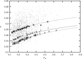
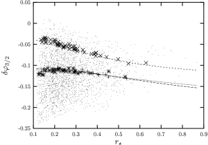
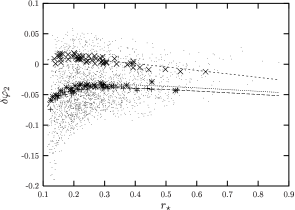
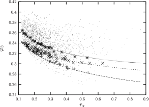
(a)

Figure 1: The overall shift $\bar{\varphi}$ (a) and the relative shifts of the first trough (b) and the second peak (c). Also given is the overall shift of the third peak (d). In all figures, the long dashed, dotted and the dashed lines represent the fitting formulae for the parameters $\left(\Omega_{b}h^{2},r^{*},n,\overline{\Omega}_{\rm ls}^{\phi}\right)=(0.02,\,r_{\star},\,1,\,0)$, $(0.02,\,r_{\star},\,1,\,0.1)$ and $(0.01,\,r_{\star},\,1,\,0)$ respectively. The large symbols show the data corresponding to these curves. The errors quoted in Appendix A are calculated from the spread of these symbols relative to the curves. The sprinkled dots represent thousands of models selected at random from the parameter space given in Table 2, and indicate the ranges of values taken on by $\bar{\varphi}$ etc. for these models.

In Sections 2 and 3 we describe a systematic procedure for extracting the acoustic scale $l_{A}$ from the location of the first three peaks. Section 4 introduces a quantity $\kappa$ which is useful as it depends only on two of our four parameters. The model (in)dependence of the fitting formulae is discussed in Section 5. Finally, our fitting formulae are given in Appendix A.

2 Retrieving the shifts from CMB measurements

With future high precision measurements of the MAP and PLANCK satellites, we expect that the position of the first three peaks and troughs will be determined to high accuracy. From these few data points, it is possible to extract valuable information on the cosmological parameters. We have observed, during our computation of CMB spectra for thousands of universes, that the overall shift of the third peak $\varphi_{3}$ (i.e. $\varphi_{3}$ $=\bar{\varphi}+\delta\varphi_{3}$) is a relatively insensitive quantity. In the parameter range we used (see Table 2) we found that $\varphi_{3}=0.341\pm 0.024$. In using $\varphi_{3}=0.341$ we introduce slight (at most one percent) systematic deviations in our estimate, because an increase of $\overline{\Omega}_{\textrm{ls}}^{\phi}$ typically increases $\varphi_{3}$ (see Fig. 1(a)). We will partially correct for these effects by improving our estimate for $\varphi_{3}$, via the procedure described below.

We start by extracting our first estimate of the overall phase shift, from the measured locations of the first and third peaks

$$\bar{\varphi}=1-(3-\varphi_{3})\frac{l_{1}}{l_{3}}\approx 1-2.66\frac{l_{1}}{l_{3}}.$$ (6)

Comparing this estimate with the value calculated from numerical simulations, we find $\Delta\bar{\varphi}=0.006$. Having a handle on the overall phase shift, it is now simple to infer the relative shifts $\delta\varphi_{m}$ of the remaining troughs and peaks. From equation (2) we get the relation

$$\delta\varphi_{m}=(m-1)-\left(\frac{l_{m}}{l_{1}}-1\right)\left(1-\bar{\varphi}\right).$$ (7)

The error of this estimate is

$$\Delta\left(\delta\varphi_{m}\right)=\left(\frac{l_{m}}{l_{1}}-1\right)\Delta\bar{\varphi}.$$ (8)

Having a first (and already quite accurate) estimate of the shifts, we now correct for the systematic effects described above. Taking the cosmological parameter set we wish to maximise over (i.e. Table 2), we calculate for each model universe the phase shifts of the first three peaks using the fitting formulae given in Appendix A. We then discard those models for which any phase shift deviates significantly (say $>2$-$\sigma$) from the data-inferred values. This leaves an improved cosmological parameter set, for which the average value of $\varphi_{3}$ is calculated (see Table 3). This improved $\varphi_{3}$ can then be used to re-calculate the phase shifts from Equations (6) and (7).

$\overline{\Omega}_{\textrm{ls}}^{\phi}$ ($\%$)		$\langle\varphi_{3}^{\rm num}\rangle$	$\langle\varphi_{3}^{\rm improved}\rangle$
0 -	2	0.313	0.326
10 -	12	0.340	0.337
18 -	20	0.362	0.348

Table 3: Binned average $\varphi_{3}$ of the numerical simulation and the improved deduction.

3 Estimating $l_{A}$

Using the improved value for $\varphi_{3}$ from the previous section, we can extract to very good accuracy the acoustic scale $l_{A}$ – the quantity which determines the overall spacing of CMB peaks:

$$l_{A}=\frac{l_{3}}{3-\varphi_{3}}$$ (9)

In fact, the deviation of the value of $l_{A}$ estimated from this formula and the numerically-obtained value is small, with a $1$-$\sigma$ error of $0.8\%$ (see also Table 4). This is a very valuable result, for the value of $l_{A}$ can be simply computed for any given quintessence (or indeed any other) cosmology. For flat universes it is given by [6]

$$l_{A}=\pi\bar{c}_{s}^{-1}\Bigg{[}\frac{F(\Omega_{\textrm{0}}^{\phi},\overline{w}_{0})}{\sqrt{1-{\overline{\Omega}_{\textrm{ls}}^{\phi}}}}\Bigg{\{}\sqrt{a_{\rm ls}+\frac{\Omega_{\textrm{0}}^{r}}{1-\Omega_{\textrm{0}}^{\phi}}}\\ -\sqrt{\frac{\Omega_{\textrm{0}}^{r}}{1-\Omega_{\textrm{0}}^{\phi}}}\Bigg{\}}^{-1}-1\Bigg{]},$$ (10)

with

$$F(\Omega_{\textrm{0}}^{\phi},\overline{w}_{0})=\frac{1}{2}\int_{0}^{1}\textrm{d}a\Bigg{(}a+\frac{\Omega_{\textrm{0}}^{\phi}}{1-\Omega_{\textrm{0}}^{\phi}}\,a^{(1-3\overline{w}_{0})}\\ +\frac{\Omega_{\textrm{0}}^{r}(1-a)}{1-\Omega_{\textrm{0}}^{\phi}}\Bigg{)}^{-1/2},$$ (11)

where $\Omega_{\textrm{0}}^{r},\Omega_{\textrm{0}}^{\phi}$ are today’s radiation and quintessence components, $a_{\rm ls}$ is the scale factor at last scattering (if $a_{0}=1$) and $\bar{c}_{s}$ is the average sound speed before last scattering:

$$\bar{c}_{s}\equiv\tau_{\rm ls}^{-1}\int_{0}^{\tau_{\rm ls}}{\rm d}\tau\left[3+(9/4)(\rho^{\rm b}(t)/\rho^{\gamma}(t))\right]^{-1/2}.$$ (12)

The effective equation of state, $\overline{w}_{0}$ is the $\Omega^{\phi}$-weighted average over conformal time

$$\overline{w}_{0}=\int_{0}^{\tau_{0}}\Omega_{\textrm{}}^{\phi}(\tau)w(\tau)\textrm{d}\tau\times\left(\int_{0}^{\tau_{0}}\Omega_{\textrm{}}^{\phi}(\tau)\textrm{d}\tau\right)^{-1}.$$ (13)

In particular, different quintessence models with the same energy density and equation of state today can have significantly different values of $l_{A}$. In this way stringent bounds on cosmological models can be imposed just by comparing the $l_{A}$ value of specific models.

4 Insensitive Quantities

The phase shifts depend on the cosmological parameters $\left(\Omega_{b}h^{2},r^{*},n,\overline{\Omega}_{\rm ls}^{\phi}\right)$. Of course, if it were possible to find a linear combination of phase shifts which is insensitive to some of these parameters and thus reduce the dimensionality of our parameter space, it would greatly help in extracting cosmological information. To this end, we note an anti-correlation between $\bar{\varphi}$ and $\delta\varphi_{3}$ – empirically, we have found that the quantity

$$\kappa\equiv\bar{\varphi}+\frac{2}{5}\delta\varphi_{3}$$ (14)

is practically insensitive to $r_{\star}$ and $\Omega_{b}h^{2}$, and depends only on $n$ and $\overline{\Omega}_{\textrm{ls}}^{\phi}$. In fact, it is to very good approximation given by the fit

$$\kappa=\left(0.277+0.284\overline{\Omega}_{\textrm{ls}}^{\phi}\right)(1.3-0.3n),$$ (15)

with $\Delta\kappa^{\rm fit}\approx 0.0024$ being the deviation of the fit from the numerically-simulated values (see Fig. 2). Following the procedure in Section 2, we can deduce $\kappa$ from the measured values of the peak locations. Within our parameter range, $\kappa$ is then determined with error $\Delta\kappa^{\rm deduc.}=0.013$.

Figure 2: The quantity $\kappa$ as a function of $r_{\star}$. It is practically insensitive to $r_{\star}$ and $\Omega_{b}h^{2}$ for most of the initial conditions considered. The dots represent fifty thousand models with parameters in the ranges given in Table 2 The $+$’s and $\times$’s represent models with $\overline{\Omega}_{\textrm{ls}}^{\phi}$ = 0 and 0.22 respectively, for $n=1$, and all values of other input parameters.

In the parameter space we have considered, the value of $\kappa$ varies between $0.26$ and $0.36$. Hence to 1-$\sigma$ confidence level, about three quarters of our two-dimensional $(n,\overline{\Omega}_{\textrm{ls}}^{\phi})$ parameter space can be excluded for any given $\kappa$. For instance, without quintessence, the value of $\kappa$ lies between $0.26$ and $0.29$ for $n\in[0.8,1.2]$. The measurement by MAP or PLANCK of a value of $\kappa>0.29$ would therefore be a strong hint of a dark energy component playing a role at last scattering.

5 Model dependence

The fitting formulae were obtained using a standard exponential potential [13] for the quintessence component. Because the shifts are almost independent of post recombination physics, we expect the results to be approximately correct for any realization of quintessence, i.e. all potentials. One should however be cautious with models that are qualitatively extremely different from the exponential potential before last scattering, as for example the Ratra-Peebles inverse power law [14] with substantial $\overline{\Omega}_{\textrm{ls}}^{\phi}$. In these models there is a sharp increase in $\Omega_{\textrm{}}^{\phi}$ during recombination, whereas the quintessence content for the exponential potential is fairly constant at this epoch.

The inverse power law is characterized by its potential $V^{\rm IPL}=A/\varphi^{\alpha}$. Models with $\alpha\gtrapprox 2$ are phenomenologically disfavoured [15]. We use these models only as cross checks for the fitting formulae.

In terms of phase shifts, one finds that the sensitive relative shifts of the first trough and the second peak differ substantially for the two models (see Table 4). However, $\bar{\varphi}$ and $\kappa$ are seen to be more robust and the deduced value of $l_{A}$ is accurate to within one percent in every case.

$\overline{\Omega}_{\textrm{ls}}^{\phi}$ ($\%$)	$l_{1}$	$l_{3/2}$	$l_{2}$	$l_{3}$	$l_{A}$	$\bar{\varphi}$	$\delta\varphi_{3/2}$	$\delta\varphi_{2}$	$\kappa$
Leaping kinetic term
3	214	396	521	788	293	0.269	-0.121	-0.045	0.287
					294	0.271	-0.119	-0.041	0.292
13	210	396	522	799	301	0.301	-0.120	-0.038	0.317
					301	0.301	-0.120	-0.038	0.318
22	208	397	524	808	307	0.324	-0.116	-0.030	0.341
					305	0.320	-0.120	-0.035	0.333
Ratra Peebles inverse power law
$5\times 10^{-3}$	199	366	480	724	269	0.259	-0.119	-0.043	0.278
					270	0.261	-0.117	-0.038	0.284
10	178	339	443	674	251	0.294	-0.140	-0.054	0.304
					253	0.298	-0.138	-0.050	0.312
22	172	338	444	683	258	0.333	-0.144	-0.057	0.340
					258	0.334	-0.145	-0.057	0.340

Table 4: The peak locations and the phase shifts of leaping kinetic term [16] and Ratra Peebles inverse power law [14] models for $\Omega_{b}h^{2}=0.021,\ \Omega_{\textrm{0}}^{\phi}=0.6,\ h=0.65,\ n=1$ and varying $\overline{\Omega}_{\textrm{ls}}^{\phi}$. The inverse power law models correspond to $\alpha=6,\,22$ and $40$ respectivly. The first row of each model gives the CMBFAST-obtained values of the locations of the peaks and the phase shifts as well as $l_{A}$ and $\kappa$. The second row gives the values deduced using the method described in Section 2.

6 Conclusions

In this paper we have shown that within a wide range of parameters, one can accurately deduce the acoustic scale $l_{A}$, as well as the shifts of the peaks and troughs provided the locations of the first three peaks are measured. Not only will this enable faster testing in likelihood analysis by providing a filter before any fluctuation equations are solved, but it could also in principle lead to a detection of quintessence – measuring a non-zero value of the dark energy at last scattering (e.g by computing the quantity $\kappa$ described in Section 4) would distinguish it from a cosmological constant, whose contribution to the energy density of the Universe would become significant only very recently.

Appendix A Fitting formulae

We present here our fitting formulae for the overall phase shift $\bar{\varphi}$, followed by the relative shifts of the first trough ($\delta\varphi_{3/2}$) and the second ($\delta\varphi_{2}$) and third ($\delta\varphi_{3}$) peaks. In each case we also give an estimate of the accuracy of the formulae.

A.1 Overall phase shift $\bar{\varphi}$

For the overall phase shift $\bar{\varphi}$ (i.e. the phase shift of the first peak) we find the formula

$$\bar{\varphi}=(1.466-0.466n)\left[a_{1}r_{\star}^{a_{2}}+0.291\overline{\Omega}_{\textrm{ls}}^{\phi}\right],$$ (16)

where $a_{1}$ and $a_{2}$ are given by

$$a_{1} = 0.286+0.626\left(\Omega_{b}h^{2}\right)$$ (17)

$$a_{2} = 0.1786-6.308\,\Omega_{b}h^{2}+174.9\left(\Omega_{b}h^{2}\right)^{2}$$ (19)

$$-1168\left(\Omega_{b}h^{2}\right)^{3}.$$

It contains the main dependence of any shift $\varphi_{m}$ on $\overline{\Omega}_{\textrm{ls}}^{\phi}$. The 1-$\sigma$ error for $\bar{\varphi}$ is

$$\Delta\bar{\varphi}=0.0031$$ (20)

A.2 Relative shift of first trough $\delta\varphi_{3/2}$

The relative shift of the first trough is a very sensitive quantity spanning a wide range of values. It can very well be used to restrict the allowed parameter space for cosmological models. We have

$$\delta\varphi_{3/2}=b_{0}+b_{1}r_{\star}^{1/3}\exp(b_{2}r_{\star})+0.158\,(n-1),$$ (21)

with

$$b_{0} = -0.086-0.079\,\overline{\Omega}_{\textrm{ls}}^{\phi}-\left(2.22-18.1\overline{\Omega}_{\textrm{ls}}^{\phi}\right)\Omega_{b}h^{2}$$ (22)

$$-\left[140+403\overline{\Omega}_{\textrm{ls}}^{\phi}\right]\left(\Omega_{b}h^{2}\right)^{2}$$

$$b_{1} = 0.39-0.98\,\overline{\Omega}_{\textrm{ls}}^{\phi}-\left(18.1-29.2\overline{\Omega}_{\textrm{ls}}^{\phi}\right)\Omega_{b}h^{2}$$ (24)

$$+440\left(\Omega_{b}h^{2}\right)^{2}$$

$$b_{2} = -0.57-3.8\exp\left\{-2365.0\left(\Omega_{b}h^{2}\right)^{2}\right\}.$$ (25)

For the one standard-deviation error we have

$$\Delta\delta\varphi_{3/2}=0.0039.$$ (26)

A.3 Relative shift of second peak $\delta\varphi_{2}$

The relative shift of the second peak is a very sensitive quantity. It is thus not surprising to find a strong dependence of $\delta\varphi_{2}$ on the parameters. We have

$$\delta\varphi_{2}=c_{0}-c_{1}r_{\star}-c_{2}r_{\star}^{-c_{3}}+0.05\,(n-1),$$ (27)

with

$$c_{0} = -0.1+\left(0.213-0.123\,\overline{\Omega}_{\textrm{ls}}^{\phi}\right)$$ (29)

$$\times\exp\left\{-\left(52-63.6\,\overline{\Omega}_{\textrm{ls}}^{\phi}\right)\Omega_{b}h^{2}\right\}$$

$$c_{1} = 0.063\,\exp\left\{-3500\left(\Omega_{b}h^{2}\right)^{2}\right\}+0.015$$ (30)

$$c_{2} = 6\times 10^{-6}+0.137\left(\Omega_{b}h^{2}-0.07\right)^{2}$$ (31)

$$c_{3} = 0.8+2.3\,\overline{\Omega}_{\textrm{ls}}^{\phi}+\left(70-126\,\overline{\Omega}_{\textrm{ls}}^{\phi}\right)\Omega_{b}h^{2}.$$ (32)

The error of this approximation is

$$\Delta\delta\varphi_{2}=0.0044.$$ (33)

A.4 Relative shift of third peak $\delta\varphi_{3}$

For the third peak, we find

$$\delta\varphi_{3}=10-d_{1}r_{\star}^{d_{2}}+0.08\,(n-1),$$ (34)

with

$$d_{1} = 9.97+\left(3.3-3\Omega_{\textrm{ls}}^{\phi}\right)\Omega_{b}h^{2}$$ (35)

$$d_{2} = 0.0016-0.0067\,\Omega_{\textrm{ls}}^{\phi}+\left(0.196-0.22\,\Omega_{\textrm{ls}}^{\phi}\right)\Omega_{b}h^{2}$$ (36)

$$+\frac{(2.25+2.77\,\Omega_{\textrm{ls}}^{\phi})\times 10^{-5}}{\Omega_{b}h^{2}},$$

and error given by

$$\Delta\delta\varphi_{3}=0.0052.$$ (37)

A.5 Overall shift of third peak $\varphi_{3}$

For completeness, we give a fit for $\varphi_{3}$ which in principle could be obtained by adding $\bar{\varphi}$ and $\delta\varphi_{3}$. However, a one-step-fit yields better errors here. Our formula is

$$\varphi_{3}=e_{1}\left(1+e_{3}r_{\star}\right)r_{\star}^{e_{2}}+e_{4}-0.037\,(n-1),$$ (38)

with

$$e_{1} = 0.302-2.112\,\Omega_{b}h^{2}+0.15\exp\left\{-384\Omega_{b}h^{2}\right\}$$ (39)

$$e_{2} = -0.04-4.5\,\Omega_{b}h^{2}$$ (40)

$$e_{3} = \left(-0.118+44.7\,\Omega_{b}h^{2}\right)\overline{\Omega}_{\textrm{ls}}^{\phi}$$ (41)

$$e_{4} = \left(0.214\exp\left\{-48\Omega_{b}h^{2}\right\}+0.106\right)\overline{\Omega}_{\textrm{ls}}^{\phi},$$ (42)

and error

$$\Delta\varphi_{3}=0.0017.$$ (43)

References

• [1] Huey, G., Wang, L., Dave, R., Caldwell, R. R., Steinhardt, P. J., 1999, Phys.Β Rev.Β D, 59, 063005 [astro-ph/9804285]
• [2] Hu, W., White, M., 1996, in Proceedings of 31st Rencontres de Moriond: Microwave Background Anisotropies, Les Arcs, France, 16-23 March 1996 (Editions Frontieres) [astro-ph/9606140]
• [3] Amendola, L., 2000, Phys.Β Rev.Β D, 62, 043511 [astro-ph/9908023]
• [4] Brax, P., Martin, J., Riazuelo, A., 2000, Phys.Β Rev.Β D, 62, 103505 [astro-ph/0005428]
• [5] Coble, K., Dodelson, S., Frieman, J. A., 1997, Phys.Β Rev.Β D, 55, 1851 [astro-ph/9608122].
• [6] Doran, M., Lilley, M. J., Schwindt. J., Wetterich, C., 2000, ApJ in press [astro-ph/0012139].
• [7] Seljak, U., Zaldarriaga, M., 1996, ApJ, 469, 437 [astro-ph/9603033]
• [8] Kamionkowski, M., Spergel, D. N., Sugiyama, N., 1994, ApJ, 426, L57 [astro-ph/9401003]
• [9] Weinberg, S., 2000, Phys.Β Rev.Β D, 62, 127302 [astro-ph/0006276]
• [10] Hu, W., Sugiyama, N., Silk, J., 1997, Nat, 386, 37 [astro-ph/9604166]
• [11] Hu, W., Fukugita, M., Zaldarriaga, M., Tegmark, M., 2000, astro-ph/0006436
• [12] Hu, W., Sugiyama, N., 1995, ApJ, 444, 489
• [13] Wetterich, C., 1988, Nucl.Β Phys.Β B, 302, 668
• [14] Peebles, P. J. E., Ratra, B., 1988, ApJ, 325, L17
• [15] A.Β Balbi, C.Β Baccigalupi, S.Β Matarrese, F.Β Perrotta and N.Β Vittorio, Astrophys.Β J.Β  547 (2001) L89
• [16] Hebecker, A., Wetterich, C., 2001, Phys.Β Lett.Β B, 497, 281 [hep-ph/0008205]