UTTG-05-01

Conference Summary
20th Texas Symposium on Relativistic Astrophysics

Steven Weinberg Department of Physics, University of Texas at Austin
weinberg@physics.utexas.edu

Abstract

This is the written version of the summary talk given at the 20th Texas Symposium on Relativistic Astrophysics in Austin, Texas, on December 15, 2000. After a brief summary of some of the highlights at the conference, comments are offered on three special topics: theories with large additional spatial dimensions, the cosmological constant problems, and the analysis of fluctuations in the cosmic microwave background.

I OVERVIEW

Speaking as a particle physicist, an outsider, I have to say that my chief reaction after a week of listening to talks at this meeting is one of envy. You astrophysicists are blessed with enlightening data in an abundance that particle physicists haven’t seen since the 1970s. And although you still face many mysteries, theory is increasingly converging with observation.

For instance, as discussed by Shri Kulkarni, it now seems clear that gamma ray bursters are at cosmological distances, producing over $10^{50}$ ergs in particle kinetic energies alone in a minute or so, making them the most spectacular objects in the sky. Tsvi Piran described a fireball model for the gamma ray bursters, in which gamma rays are produced by relativistic particles accelerated by shocks within material that is ejected ultra-relativisticaly from a central source. One can think of various mechanisms for the hidden central source, but even without a specific model for the source, the fireball model does a good job of accounting for what is observed.

According to this fireball model, gamma rays from the bursters are strongly beamed. Peter Höflich presented evidence that core collapse supernova are also highly aspherical. Both conclusions may be good news for gravitational wave astronomers — only aspherical explosions can generate gravitational waves.

Spectacular things seem to be turning up all over. Amy Barger told us how X-ray observations are revealing many active galactic nuclei in what had previously seemed like ordinary galaxies, and John Kormendy reported evidence that the events that produce galactic bulges or elliptical galaxies are the same as those that produce black holes in galactic centers.

Astrophysics is currently the beneficiary of massive surveys that are providing or will soon provide a flood of important data. We heard from John Peacock about the 2dF Galaxy Redshift Survey, from Bruce Margon about the Sloan Digital Sky Survey, and from George Ricker about the HETE x-ray and $\gamma$ - ray satellite mission. Together with cosmic microwave background observations, about which more later, there seems to be a general consistency with the big bang cosmology, with about 30% of the critical mass furnished by cold dark matter, and about $70\%$ furnished by negative-pressure vacuum energy.

This is not to say that there are no puzzles. Alan Watson reported on the long-standing puzzles of understanding how the highest energy cosmic rays are generated and how they manage to get to earth through the cosmic microwave background. There are also persistent problems in matching the cold dark matter model to observations of the mass distribution in galaxies. Ben Moore cast some doubt on whether cold dark matter really leads to the missing “cuspy cores” of galaxy haloes, and he concentrated instead on a different problem: cold dark matter models give much more matter in satellites of galaxies than is observed. He suggests that the missing satellites may really be there, and that they have not been observed because they have not formed stars. The reionization processes discussed here by Paul Shapiro may be responsible for the failure of star formation.

Our knowledge of the dark matter mass distribution within galaxies is receiving important contributions from observations of the lensing of quasar images by intervening galaxies, discussed by Genevieve Soucail. There have been hopes of using surveys of gravitational lenses to distinguish among cosmological models, but I have the impression that the study of galactic lenses will turn out to be more important in learning about the lensing galaxies themselves. Andrew Gould reported that microlensing observations have ruled out the dark matter being massive compact halo objects with masses in the range $10^{-7}M_{\odot}$ to $10^{-3}M_{\odot}$ .

It would of course be a great advance if cold dark matter particles could be directly detected. We heard a lively debate about whether weakly interacting massive dark matter particles have already been detected, between Rita Bernabei (pro) and Blas Cabrera (con). It would be foolhardy for a theorist to try to judge this issue, but at least one gathers that, if the dark matter is composed of WIMPs, then they can be detected.

I have now completed my 10 minute general summary of the conference. There were other excellent plenary talks, and I have not mentioned any of the parallel talks, but what can you do in 10 minutes? In the remaining 35 minutes, I want to take up some special topics, on which I will have a few comments of my own.

II LARGE EXTRA DIMENSIONS

It is an old idea that the four spacetime dimensions in which we live are embedded in a higher dimensional spacetime, with the extra dimensions rolled up in some sort of compact manifold with radius $R$ . This would have profound cosmological consequences: the compactification of the extra dimensions could be the most important event in the history of the universe, and such theories would contain vast numbers of new types of particle.

In the original version of this theory any field would have normal modes that would be observed in four dimensions as an infinite tower of ‘Kaluza–Klein recurrences,’ particles carrying the quantum numbers of the fields, with masses given by multiples of $1/R$ . It had generally been supposed that $R$ would be of the order of the Planck length, or perhaps 10 to 100 times larger, of the order of the inverse energy $M$ at which the strong and electroweak coupling constants are unified. Even setting this preconception aside, it had seemed that in any case $R$ would have to be smaller than $10^{-16}\;{\rm cm}\approx(100\;{\rm GeV})^{-1}$ , in order that the Kaluza–Klein recurrences of the particles of the standard model would be heavy enough to have escaped detection.

The possibilities for higher dimensional theories became much richer with the increasing attention given to the idea that the spacetime in which we live does not merely appear four-dimensional — our three-space may be a truly three-dimensional surface that is embedded in a higher dimensional space. (This is the picture of higher dimensions that was vividly described in Edwin Abbott’s 1884 novel Flatland, and has more recently become an important part of string theory, starting with Polchinski’s work on D-branes[1].) This idea opens up the possibility that some fields may depend only on position on the four-dimensional spacetime surface, while others ‘live in the bulk’ — that is, they depend on position in the full higher-dimensional space. Only the fields that live in the bulk would have Kaluza–Klein recurrences.

Craig Hogan here discussed the recently proposed idea that the compactification scale $R$ may actually be much larger than $10^{-16}$ cm, with no Kaluza–Klein recurrences for the particles of the standard model because the standard model fields depend only on position in the four-dimensional spacetime in which we live[2]. According to this idea, it is only the gravitational field that depends on position in the higher dimensional space, and so it is only the graviton that has has Kaluza–Klein recurrences, which at ordinary energies would interact too weakly to have been observed. The long range forces produced by exchange of these massive gravitons would be small enough to have escaped detection in measurements of gravitational forces between laboratory masses as long as $R<1$ mm. (There are stronger astrophysical and cosmological bounds on $R$ , arising from limits on the production of graviton recurrences in supernovas[3] and in the early universe[4].)

In any such theory with large compactification radius $R$ the Planck mass scale of the higher dimensional theory of gravitation would be very much less than the Planck mass scale in our four dimensional spacetime. In a world with $4+N$ spacetime dimensions the gravitational constant $G_{4+N}$ (the reciprocal of the coefficient of the term $\int d^{4+N}x\,\sqrt{g}\,g_{\mu\nu}R^{\mu\nu}$ in the action) has dimensionality $[{\rm mass}]^{-2-N}$ , so we would expect it to be given in terms of some fundamental higher dimensional Planck mass scale $M_{*}$ by $G_{4+N}\approx M_{*}^{-2-N}$ . Dimensional analysis then tells us that the gravitational constant $G$ in four spacetime dimensions must be given by

G\approx M_{*}^{-2-N}R^{-N}\;.

(1)

The usual assumption in theories with extra dimensions has been that $R\approx M_{*}^{-1}$ , in which case $G\approx M_{*}^{-2}$ , and $M_{*}$ would have to be about $10^{19}$ GeV. But if we take $N=1$ and $R\approx$ 1 mm, then $1/R\approx 10^{-13}$ GeV, and $M_{*}\approx 10^{8}$ GeV. With $N=2$ and $R\approx$ 1 mm, $M_{*}\approx 300$ GeV. This is the most attractive aspect of theories with large extra dimensions: they can reduce or eliminate what had seemed like a huge gap between the characteristic energy scale of electroweak symmetry breaking and the fundamental energy scale at which gravitation becomes a strong interaction.

Theories with large extra dimensions are very ingenious, and they may even be correct, but I am not enthusiastic about them, for they give up the one solid accomplishment of previous theories that attempt to go beyond the standard model: the renormalization group equations of the original standard model showed that there is an energy, around $10^{15}$ GeV, where the three independent gauge coupling constants become nearly equal[5]. In the supersymmetric version of the standard model the convergence of the couplings with each other becomes more precise[6], and the energy scale $M_{U}$ of this unification moves up to about $2\times 10^{16}$ GeV [7], which is less than would be expected in string theories of gravitation by a factor of only about 20. (This is also a plausible energy scale for the violation of lepton number conservation that may be showing up in the neutrino oscillation experiments discussed here by Masayuki Nakahata.) The Kaluza–Klein tower of graviton recurrences does nothing to change the running of the strong and electroweak coupling constants, and since the higher dimensional Planck mass $M_{*}$ is very much less than $10^{15}$ GeV in theories with large extra dimensions (this, after all, is the point of these theories), it appears that in these theories the standard model gauge couplings are not unified at the fundamental mass scale $M_{*}$ . Of course, they might be unified at some higher energy, but we have no way to calculate what happens in these theories at any energy higher than $M_{*}$ .

In his talk here Hogan mentioned that Dienes, Dudas, and Gherghetta[8] have proposed a way out of this problem. I looked up their papers, and found that they modify the renormalization group equations for the gauge couplings of the standard model by allowing the gauge and Higgs fields (and perhaps some fermion fields) to depend on position in the higher dimensional space, along with the gravitational field. Of course, then they have to avoid conflict with experiment by taking $1/R$ greater than 100 GeV. The Kaluza-Klein recurrences of the gauge bosons greatly increase the rate at which the coupling constants of the standard model run, but with little change in their unification. To put this quantitatively, Dienes et al. find the bare (Wilsonian) couplings evaluated with a cut-off $\Lambda$ are

\frac{4\pi}{g_{i}^{2}(\Lambda)}=\frac{4\pi}{g_{i}^{2}(m_{Z})}-\frac{b_{i}}{2\pi}\ln\frac{\Lambda}{m_{Z}}+\frac{\bar{b}_{i}}{2\pi}\ln\Lambda R-\frac{\bar{b}_{i}X_{N}}{2\pi N}\left[(\Lambda R)^{N}-1\right]\;,

(2)

where $g_{1}$ and $g_{2}$ are defined as usual in terms of the electron charge $e$ and the electroweak mixing angle $\theta$ by $g^{2}_{1}=e^{2}/\sin^{2}\theta$ and $g^{2}_{2}=5e^{2}/3\cos^{2}\theta$ ; $g_{3}$ is the coupling constant of quantum chromodynamics; and $X_{N}$ is a number of order unity. The constants $(b_{1},b_{2},b_{3})$ are the factors $(33/5,1,-3)$ appearing in the renormalization group equation of the supersymmetric standard model with two Higgs doublets, while the constants $(\bar{b}_{1},\bar{b}_{2},\bar{b}_{3})$ are the corresponding factors $(3/5,-3,-6)$ in the renormalization group equations for $\Lambda$ above the compactification scale $1/R$ (with a possible constant added to each of the $\bar{b}_{i}$ , proportional to the number of chiral fermions that live in the bulk). Dienes et al. remark that the standard model couplings still come close to converging to a common value, because the ratios of the differences of the $\bar{b}_{i}$ are not very different from the ratios of the differences of the $b_{i}$ . I would like to put this more quantitatively, by asking what value of $\sin^{2}\theta$ is needed in order for the couplings to become exactly equal at some value of $\Lambda$ . In the supersymmetric standard model, this is

\sin^{2}\theta=\frac{3(b_{3}-b_{2})+5(b_{2}-b_{1})e^{2}/g_{3}^{2}}{8b_{3}-3b_{2}-5b_{1}}=\frac{1}{5}+\frac{7}{15}\frac{e^{2}}{g_{3}^{2}}=0.231\;,

(3)

in excellent agreement with the measured value $0.23117\pm 0.00016$ . (Here $e$ and $g_{3}$ are taken as measured at $m_{Z}$ , in which case $e^{2}/4\pi=1/128$ and $g_{3}^{2}/4\pi=0.118$ .) If all the running of the couplings were at scales greater than $1/R$ , then $\sin^{2}\theta$ would be given by Eq. (3), but with $b_{i}$ replaced with $\bar{b}_{i}$ :

\sin^{2}\theta=\frac{3(\bar{b}_{3}-\bar{b}_{2})+5(\bar{b}_{2}-\bar{b}_{1})e^{2}/g_{3}^{2}}{8\bar{b}_{3}-3\bar{b}_{2}-5\bar{b}_{1}}=\frac{3}{14}+\frac{3}{7}\frac{e^{2}}{g_{3}^{2}}=0.243\;.

(4)

This is not bad, but nevertheless outside experimental bounds. (It would be necessary to consider higher-order contributions in the renormalization group equations and threshold effects to be sure that there is really a discrepancy here.) In order not to spoil the prediction for $\sin^{2}\theta$ , $1/R$ would have to be considerably larger than 1 TeV, so that much of the running of the coupling constants would occur at scales below $1/R$ , where the renormalization group equations are those of the supersymmetric standard model.

In any case, the running of the couplings is so rapid above the compactification scale $1/R$ that the couplings become equal (to the extent that they do become equal) at an energy not far above $1/R$ . The $4+N$ dimensional Planck scale $M_{*}$ given by Eq. (1) is very much greater than this. Taking $1/R$ greater than 1 TeV, Eq. (1) would give $M_{*}$ greater than $10^{13}$ GeV for $N=1$ . Even for $N=7$ , we would have $M_{*}$ greater than $10^{6}$ GeV. Thus theories of this sort save the unification of couplings at the cost of reintroducing a large gap between the higher-dimensional Planck scale $M_{*}$ and the electroweak scale.

III VACUUM ENERGY

There are now two problems surrounding the energy of empty space[9]. The first is the old problem, why the vacuum energy density is so much smaller than any one of a number of individual contributions. For instance, it is smaller than the energy density in quantum fluctuations of the gravitational field at wavelengths above the Planck length by a factor of about $10^{-122}$ and it is smaller than the latent heat associated with the breakdown of chiral symmetry in the strong interactions by a factor about $10^{-50}$ . All these contributions can be cancelled by just adding an appropriate cosmological constant in the gravitational field equations; the problem is why there should be such a fantastically well-adjusted cancellation. The second, newer, problem is why the vacuum energy density that seems to be showing up in supernova studies of the redshift-distance relation (reviewed in a parallel session by Nick Suntzeff and Saul Perlmutter) is of the same order of magnitude (apparently larger by a factor about 2) as the matter density at the present time. There are five broad classes of attempts to solve one or both of these problems:

1) Cancellation Mechanisms
It has occurred to many theorists that the gravitational effect of vacuum energy might be wiped out by the dynamics of a scalar field, which automatically adjusts itself to minimize the spacetime curvature. So far, this has never worked. Some recent attempts were described by Andre Linde in a parallel session.

2) Deep Symmetries
There are several symmetries that could account for a vanishing vacuum energy, if they were not broken. One is scale invariance; another is supersymmetry. The problem is to see how to preserve the vanishing of the vacuum energy despite the breakdown of the symmetry. No one knows how to do this.

3) Quintessence
It is increasingly popular to consider the possibility that the vacuum energy is not constant, but evolves with the universe[10]. For instance, a real scalar field $\phi$ with Lagrangian density $-\partial_{\mu}\phi\partial^{\mu}\phi/2-V(\phi)$ if spatially homogeneous contributes a vacuum energy density and a pressure

\rho=\frac{1}{2}\dot{\phi}^{2}+V(\phi)\;,~{}~{}~{}~{}~{}~{}~{}p=\frac{1}{2}\dot{\phi}^{2}-V(\phi)\;,

(5)

so the condition $\rho+3p<0$ for an accelerating expansion is satisfied if the field $\phi$ is evolving sufficiently slowly so that $\dot{\phi}^{2}<V(\phi)$ .

It must be said from the outset that, in themselves, quintessence theories do not help with the first problem mentioned above — they do not explain why $V(\phi)$ does not contain an additive constant of the order of $(10^{19}{\rm GeV})^{4}$ . It is true that superstring theories naturally lead to “modular” scalar fields $\phi$ for which $V(\phi)$ does vanish as $\phi\rightarrow\infty$ , in which case the vacuum becomes supersymmetric. It might be hoped that the vacuum energy is small now, because the scalar field is well on its way toward this limit. The trouble is that the vacuum now is nowhere near supersymmetric, so that in these theories we would expect a present vacuum energy of the order of the fourth power of the supersymmetry-breaking scale, or at least $(1\;{\rm TeV})^{4}$ .

On the other hand, such theories may help with the second problem, if the quintessence energy is somehow related to the energy in matter and radiation, because the present moment is not so many $e$ -foldings of cosmic expansion (about 10, in fact) from the turning point in cosmic history when the radiation energy density (including neutrinos) fell below the matter energy density. Paul Steinhardt here described a model in which the quintessence energy density was less than the radiation energy density by a constant factor $r$ , as long as radiation dominated over matter[11]. (It is necessary that $r$ be considerably less than unity, in order that quintessence should not appreciably increase the expansion rate during the era of nucleosynthesis, increasing the present helium abundance above the observed value.) Then when the radiation energy density fell below the matter energy density at a cross-over redshift $z_{C}\approx 3000$ the quintessence energy dropped sharply by a factor of order $r^{2}$ , and has remained roughly constant since then. Since the cross-over between radiation and matter dominance the matter energy density has decreased by a factor $z_{C}^{-3}$ , so the ratio of the quintessence energy density and the matter energy density now should be of order $r^{2}\times r\times z_{C}^{3}=(z_{C}r)^{3}$ . For the quintessence and matter energies to be about equal now, $r$ must be equal to about $1/z_{C}\approx 3\times 10^{-4}$ . Steinhardt tells me that when these calculations are done carefully, the required ratio $r$ of quintessence to radiation energy density at early times is about $10^{-2}$ , rather than $3\times 10^{-4}$ . But whatever the value of $r$ that makes the quintessence energy comparable to the matter energy density now, it requires some fairly fine tuning: changing $r$ by a factor $10$ would change the ratio of the present values of the quintessence energy density and the matter energy density by a factor $10^{3}$ .

4) Brane Solutions

Several authors have found solutions of brane theories of the Randall–Sundrum kind[2] in which our four-dimensional spacetime is flat, despite the presence of a large cosmological constant in the higher dimensional gravitational Lagrangian[12]. These solutions contained an unacceptable essential singularity off the brane, but there are models in which this can be avoided[13]. I don’t believe that there is anything unique in these solutions, so that instead of having to fine tune parameters in the Lagrangian one has to fine tune initial conditions. Also, it is not clear why the effective cosmological constant has to be zero now, rather than before the spontaneous breakdown of the chiral symmetry of quantum chromodynamics, when the latent heat associated with this phase transition would have given the vacuum an energy density $(1\;{\rm GeV})^{4}$ .

5) Anthropic Principle
Why is the temperature on earth in the narrow range where water is liquid? One answer is that otherwise we wouldn’t be here. This answer makes sense only because there are many planets in the universe, with a wide range of surface temperatures. Because there are so many planets, it is natural that some of them should have liquid water, and of course it is just these planets on which there would be anyone to wonder about the temperature. In the same way, if our big bang is just one of many big bangs, with a wide range of vacuum energies, then it is natural that some of these big bangs should have a vacuum energy in the narrow range where galaxies can form, and of course it is just these big bangs in which there could be astronomers and physicists wondering about the vacuum energy. To be specific, a constant vacuum energy if negative would have to be greater than about $-10^{-120}m_{\rm Planck}^{4}$ , in order for the universe not to collapse before life has had time to develop[14], and if positive it would have to be less than about $+10^{-118}m_{\rm Planck}^{4}$ , in order for galaxies to have had a chance to form before the matter energy density fell too far below the vacuum energy density[15]. As far as I know, this is at present the only way of understanding the small value of the vacuum energy. But of course it makes sense only if the big bang in which we live is one of an ensemble of many big bangs with a wide range of values of the cosmological constant. There are various ways that this might be realized:

: (a) Wormholes or other quantum gravitational effects may cause the wave function of the universe to break up into different incoherent terms, corresponding to various possible universes with different values for what are usually called the constants of nature, perhaps including the cosmological constant[16].
: (b) Various versions of “new” inflation lead to a continual production of big bangs[17], perhaps with different values of the vacuum energy. For instance, if there is a scalar field that takes different initial values in the different big bangs, and if it has a sufficiently flat potential, then its energy appears like a cosmological constant, which takes different values in different big bangs[18].
: (c) As the universe evolves the vacuum energy may drop discontinuously to lower and lower discrete values. One way for this to happen is for the vacuum energy to be a function of a scalar field, with many local minima, so that as the universe evolves the vacuum energy keeps dropping discontinuously to lower and lower local minima[19]. Another possibility[20] with similar consequences is based on the introduction of an antisymmetric gauge potential $A_{\mu\nu\lambda}$ , which enters in the Lagrangian density in a term proportional to $F^{\mu\nu\lambda\kappa}F_{\mu\nu\lambda\kappa}$ , where $F_{\mu\nu\lambda\kappa}$ is $\partial_{\kappa}A_{\mu\nu\lambda}$ with antisymmetrized indices. Instead of a scalar field tunneling from one minimum of a potential to another, the vacuum energy evolves through the formation of membranes, across which there is a discontinuity in the value of Lorentz-invariant gauge fields $F_{\mu\nu\lambda\kappa}=F\epsilon_{\mu\nu\lambda\kappa}$ . To allow an anthropic explanation of the smallness of the vacuum energy, it is essential that the metastable values of the vacuum energy be very close together. Several models of this sort have been proposed recently[21].

Under any of these alternatives, we have not only an upper bound[15] on the vacuum energy density, given by the matter energy density at the time of formation of the earliest galaxies, but also a plausible expectation, which Vilenkin calls the principle of mediocrity[22], that the vacuum energy density found by typical astronomers will be comparable to the mass density at the time when most galaxies condense, since any larger vacuum energy density would reduce the number of galaxies formed, and there is no reason why the vacuum energy density should be much smaller. The observed vacuum energy density is somewhat smaller than this, but not very much smaller. This can be put quantitatively[23]: under the assumption[24] that the a priori probability distribution of the vacuum energy is approximately constant within the narrow range within which galaxies can form, the probability that an astronomer in any of the big bangs would find a value of $\Omega_{\Lambda}$ as small as $0.7$ ranges from 5% to 12%, depending on various assumptions about the initial fluctuations. In this calculation the fractional fluctuation in the cosmic mass density at recombination is assumed to take the value observed in our big bang, since the vacuum energy would have a negligible effect on physical processes at and before recombination. There are also interesting calculations along these lines in which the rms value of density fluctuations at recombination is allowed to vary independently of the vacuum energy[25].

IV COSMIC MICROWAVE BACKGROUND ANISOTROPIES

Perhaps the most remarkable improvement in cosmological knowledge over the past decade has been in studies of the cosmic microwave background. Since COBE, there is for the first time a cosmological parameter — the radiation temperature — that is known to three significant figures. More recently, since the BOOMERANG and MAXIMA experiments reviewed here by Paolo de Bernardis, our knowledge of small angular scale anisotropies has become good enough to set useful limits on other cosmological parameters, such as the present spatial curvature.

Unfortunately, this has produced a frustrating situation for those of us who are not specialists in the theory of the cosmic microwave background. We see papers in which experimental results for the strengths $C_{\ell}$ of the $\ell$ th multipole in the temperature correlation function are compared with computer generated plots of $C_{\ell}$ versus $\ell$ for various values of the cosmological parameters, without the non-specialist reader being able to understand why the theoretical plots of $C_{\ell}$ versus $\ell$ look the way they do, or why they depend on cosmological parameters the way they do. I want to take the opportunity here to advertise a formalism[26] that I think helps in understanding the main features of the observed anisotropies, and how they depend on various cosmological assumptions.

One can show under very general assumptions that the fractional variation from the mean of the cosmic microwave background temperature observed in a direction $\hat{n}$ takes the form

\frac{\Delta T(\hat{n})}{T}=\int d^{3}k\,\epsilon_{\bf k}\,e^{id_{A}{\bf k}\cdot\hat{n}}\,\left[F(k)+i\,\hat{n}\cdot\hat{k}\,G(k)\right]\;,

(6)

where $d_{A}$ is the angular diameter distance of the surface of last scattering

d_{A}=\frac{1}{\Omega_{C}^{1/2}H_{0}(1+z_{L})}\sinh\left[\Omega_{C}^{1/2}\int_{\frac{1}{1+z_{L}}}^{1}\frac{dx}{\sqrt{\Omega_{\Lambda}x^{4}+\Omega_{C}x^{2}+\Omega_{M}x}}\right]\;,

(7)

(with $z_{L}\simeq 1100$ and $\Omega_{C}\equiv 1-\Omega_{M}-\Omega_{V}$ ); ${\bf k}^{2}\epsilon_{\bf k}$ is proportional to the Fourier transform of the fluctuation in the energy density at early times (with ${\bf k}$ the physical wave number vector at the nominal moment of last scattering, so that $d_{A}{\bf k}$ in the argument of the exponential is essentially independent of how this moment is defined); and $F(k)$ and $G(k)$ are a pair of form factors that incorporate all relevant information about acoustic oscillations up to the time of last scattering, with $F(k)$ arising from intrinsic temperature fluctuations and the Sachs–Wolfe effect, and $G(k)$ arising from the Doppler effect. Given the form factors, one can find the coefficients $C_{\ell}$ for $\ell\gg 1$ by a single integration

\ell(\ell+1)C_{\ell}\rightarrow\frac{8\pi^{2}\ell^{3}}{d_{A}^{3}}\int_{1}^{\infty}d\beta\,{\cal P}(\ell\beta/d_{A})\left[\frac{\beta F^{2}(\ell\beta/d_{A})}{\sqrt{\beta^{2}-1}}+\frac{\sqrt{\beta^{2}-1}\,G^{2}(\ell\beta/d_{A})}{\beta}\right]\;.

(8)

where ${\cal P}(k)$ is the power spectral function, defined by

\left\langle\epsilon_{\bf k}\,\epsilon_{\bf k^{\prime}}\right\rangle=\delta^{3}({\bf k}+{\bf k^{\prime}})\,{\cal P}(k)\;.

(9)

(The first term in the square brackets in Eq. (8) appeared in a calculation by Bond and Efstathiou[27]; I think the second is new.)

As you can see from the $F^{2}(k)$ term in Eq. (8), for $\ell\gg 1$ the main contribution to $C_{\ell}$ of the Sachs–Wolfe effect and intrinsic temperature fluctuations comes from wave numbers close to $d_{A}/\ell$ , but this well-known result is not a good approximation for the Doppler effect form factor $G(k)$ . Since it is the form factors rather than $C_{\ell}$ that really reflect what was going on before-recombination, it is important to try to measure them more directly, as for instance through interferometric measurements of the temperature correlation function, of the sort described in a parallel session by K. Y. Lo et al. and B. S. Mason et al.

The Harrison–Zel’dovich spectrum suggested by theories of new inflation[28] is ${\cal P}(k)=Bk^{-3}$ , with $B$ a constant. In this case Eq. (8) gives a formula for $C_{\ell}$ that is valid for $\ell\gg 1$ and $\ell\ll d_{A}/d_{H}$ (where $d_{H}\ll d_{A}$ is the horizon distance at the time of last scattering):

\ell(\ell+1)C_{\ell}\rightarrow 8\pi^{2}BF_{0}^{2}\left\{1-\frac{\ell^{2}}{d_{A}^{2}}\left[d^{2}\,\left(\ln\left(\frac{\bar{d}\,\ell}{2d_{A}}\right)-C\right)-d^{\prime 2}\right]+\dots\right\}\;,

(10)

where $C$ is the Euler constant $C\equiv-\Gamma^{\prime}(1)=0.57722$ , and $d$ and $d^{\prime}$ are a pair of characteristic lengths of order $d_{H}$ :

d^{2}\equiv\frac{2F_{0}F_{2}+G_{1}^{2}}{F^{2}_{0}}\;,~{}~{}~{}~{}~{}~{}d^{\prime 2}\equiv\frac{3F_{0}F_{2}+\frac{1}{2}G_{1}^{2}}{F^{2}_{0}}\;,

(11)

expressed in terms of coefficients in a power series expansion of the form factors:

F(k)=F_{0}+F_{2}\,k^{2}+\cdots\;,~{}~{}~{}~{}~{}~{}~{}~{}G(k)=G_{1}k+G_{3}k^{3}+\cdots\;.

(12)

(This formula applies even when $\ell$ is not much larger than unity, except for $\ell=0$ and $\ell=1$ [29], provided we replace $\ell^{2}$ with $\ell(\ell+1)$ and $\ln\ell$ with $\sum_{r=1}^{\ell}1/r+C$ .) The quantity $\bar{d}$ in the logarithm is another length of order $d_{H}$ , this one given by a much more complicated expression involving the form factors at all wave numbers, but since $d_{H}\ll d_{A}$ the precise value of $\ln(\bar{d}/2d_{A})$ does not depend sensitively on the precise value of $\bar{d}$ .

One advantage of this formalism is that it provides a nice separation between the three different kinds of effect that influence the observed temperature fluctuation, that arise in three different eras: the power spectral function ${\cal P}(k)$ characterizes the origin of the fluctuations, perhaps in the era of inflation; the form factors $F(k)$ and $G(k)$ characterize acoustic fluctuations up to the time of last scattering; and the angular diameter distance $d_{A}$ depends on the propagation of light since then. This allows us to see easily what depends on what parameters. The form factors $F(k)$ and $G(k)$ depend strongly on $\Omega_{B}h^{2}$ (through the effect of baryons on the sound speed) and more weakly on $\Omega_{M}h^{2}$ (through the effect of radiation on the expansion rate before the time of last scattering), but since the curvature and vacuum energy were negligible at and before last scattering, $F(k)$ and $G(k)$ are essentially independent of the present curvature and of $\Omega_{\Lambda}$ . The power spectral function ${\cal P}(k)$ is expected to be independent of all these parameters. On the other hand, $d_{A}$ is affected by whatever governed the paths of light rays since the time of last scattering, so it depends strongly on $\Omega_{M}$ , $\Omega_{\Lambda}$ , and the spatial curvature, but it is essentially independent of $\Omega_{B}$ . In quintessence theories $d_{A}$ would be given by a formula different from (7), but ${\cal P}(k)$ and the form factors would be essentially unchanged as long as the quintessence energy density was a small part of the total energy density at and before the time of last scattering. In particular, Eq. (8) shows that $\ell(\ell+1)C_{\ell}$ for $\ell\gg 1$ depends on $\ell$ and $d_{A}$ only through the ratio $\ell/d_{A}$ , so changes in $\Omega_{\Lambda}$ or the introduction of quintessence would lead to a re-scaling of all the $\ell$ -values of the peaks in the plots of $\ell(\ell+1)C_{\ell}$ versus $\ell$ , but would have little effect on their height.

Refer to caption — Figure 1: Plots of the ratio of the multipole strength parameter $\ell(\ell+1)C_{\ell}$ to its value at small $\ell$ , versus $\ell d_{H}/d_{A}$ , where $d_{H}$ is the horizon size at the time of last scattering and $d_{A}$ is the angular diameter distance of the surface of last scattering. The curves are for $\Omega_{B}h^{2}$ ranging (from top to bottom) over the values 0.03, 0.02, 0.01, and 0, corresponding to $\xi$ taking the values 0.81, 0.54, 0.27, and 0. The solid curves are calculated using the WKB approximation; dashed lines indicate an extrapolation to the known value at small $\ell d_{H}/d_{A}$ .

Another advantage of this formalism is that, although $C_{\ell}$ must be calculated by a numerical integration, it is possible to give approximate analytic expressions for the form factors in terms of elementary functions, at least in the approximation that the dark matter dominates the gravitational field for a significant length of time before last scattering. (There have been numerous earlier analytic calculations of the temperature fluctuations[30], and their results may all be put in the form (6), but my point here is that this form is general, not depending on the particular approximations used.) In this approximation the form factors for very small wave numbers are

	$\displaystyle F(k)$	$\displaystyle\rightarrow$	$\displaystyle 1-3k^{2}t_{L}^{2}/2-3[-\xi^{-1}+\xi^{2}\ln(1+\xi)]k^{4}t_{L}^{4}/4+\dots\;,$		(13)
	$\displaystyle G(k)$	$\displaystyle\rightarrow$	$\displaystyle 3kt_{L}-3k^{3}t_{L}^{3}/2(1+\xi)+\dots\;,$		(14)

while for wave numbers large enough to allow the use of the WKB approximation the form factors are

F(k)=(1+2\xi/k^{2}t_{L}^{2})^{-1}\left[-3\xi+2\xi/k^{2}t_{L}^{2}+(1+\xi)^{-1/4}e^{-k^{2}d_{\Delta}^{2}}\cos(kd_{H})\right]\;,

(15)

and

G(k)=\sqrt{3}\,(1+2\xi/k^{2}t_{L}^{2})^{-1}(1+\xi)^{-3/4}e^{-k^{2}d_{\Delta}^{2}}\sin(kd_{H})\;.

(16)

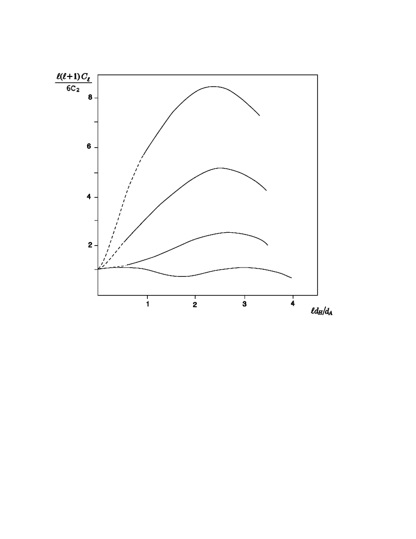
Here $t_{L}$ is the time of last scattering; $\xi=27\Omega_{B}h^{2}$ is $3/4$ the ratio of the baryon to photon energy densities at this time; $d_{H}$ is the acoustic horizon size at this time; and $d_{\Delta}$ is a damping length, typically less than $d_{H}$ . Using these results in Eq. (8) gives the curves for $\ell(\ell+1)C_{\ell}/6C_{2}$ versus $\ell d_{H}/d_{A}$ shown in Figure 1, in the approximation that damping and the term $2\xi/k^{2}t_{L}^{2}$ may be neglected near the peak. In this approximation the scalar form factor $F(k)$ has a peak at $k_{1}=\pi/d_{H}$ for any value of $\Omega_{B}h^{2}$ , but the peak in $\ell(\ell+1)C_{\ell}$ does not appear (as is often said) at $\ell=k_{1}d_{A}=\pi d_{A}/d_{H}$ ; instead, $\ell d_{H}/d_{A}$ at the peak ranges from 3.0 to 2.6, depending on the value of $\Omega_{B}h^{2}$ .

We see even from these crude calculations how sensitive is the height of the first peak in $\ell(\ell+1)C_{\ell}/6C_{2}$ to the baryon density parameter $\Omega_{B}h^{2}$ . (The experimental value[31] for the height of this peak is about 6.) Right now, there is some worry about the fact that the value of $\Omega_{B}h^{2}$ inferred from the ratio of the heights of the second and first peaks is larger than that inferred from considerations of cosmological nucleosynthesis. Perhaps it would be worth trying to estimate $\Omega_{B}h^{2}$ by comparing theory and experiment for the ratio of $\ell(\ell+1)C_{\ell}$ at the first peak to its value for small $\ell$ , discarding the data at the second peak where the statistics are worse and complicated damping effects make the theory more complicated.¹¹1At the meeting someone in the audience said that this has been done, but that was in the early days, not I think with the more detailed information now available.

ACKNOWLEDGMENTS

I am grateful to Willy Fischler, Hugo Martel, Paul Shapiro, and Craig Wheeler for their help in preparing this report. This research was supported in part by a grant from the Welch Foundation and by National Science Foundation Grants PHY 9511632 and PHY 0071512.

REFERENCES