Timescale Stretch Parameterization of Type Ia Supernova $B$-band Light Curves

Abstract

$R$-band intensity measurements along the light curve of Type Ia supernovae discovered by the Supernova Cosmology Project (SCP) are fitted in brightness to templates allowing a free parameter the time-axis width factor $w\equiv s\times(1+z)$. The data points are then individually aligned in the time-axis, normalized and $K$-corrected back to the rest frame, after which the nearly 1300 normalized intensity measurements are found to lie on a well-determined common rest-frame $B$-band curve which we call the “composite curve”. The same procedure is applied to 18 low-redshift Calán/Tololo SNe with $z<0.11$; these nearly 300 $B$-band photometry points are found to lie on the composite curve equally well. The SCP search technique produces several measurements before maximum light for each supernova. We demonstrate that the linear stretch factor, $s$, which parameterizes the light-curve timescale appears independent of $z$, and applies equally well to the declining and rising parts of the light curve. In fact, the $B$ band template that best fits this composite curve fits the individual supernova photometry data when stretched by a factor $s$ with $\chi^{2}/DoF$ $\approx$ 1, thus as well as any parameterization can, given the current data sets. The measurement of the date of explosion, however, is model dependent and not tightly constrained by the current data. We also demonstrate the $1+z$ light-curve time-axis broadening expected from cosmological expansion. This argues strongly against alternative explanations, such as tired light, for the redshift of distant objects.

1 Introduction

In systematic searches over the last 12 years the Supernova Cosmology Project (SCP) has discovered and studied over 100 supernovae, most of which have been spectroscopically identified as Type Ia supernovae (SNe Ia) at redshifts up to $z=1.20$. Forty-two of these events have so far been used for measurements of the cosmological parameters $\Omega_{M}$ and $\Omega_{\Lambda}$ (Perlmutter et al. (1999), hereafter “P99”; see also Perlmutter et al. 1995 and 1997, hereafter “P95” and “P97”). See also Riess et al. 1998 who used sixteen high redshift SNe in a parallel study of the cosmological parameters. An important element of these studies has been the recognition of homogeneity within a one parameter family of SN Ia light curves.

Several approaches have been used to characterize the SN Ia light-curve family. Phillips (1993) first suggested that the range of SNe Ia light curves might be grouped into a single family of curves parameterized by their initial rate of decline (see also the earlier suggestions of Pskovskii (1977, 1984)). Phillips (1993) and Hamuy et al. (1995) further observed that the absolute magnitudes of SNe Ia at maximum light were tightly correlated with this decline rate in the $B$-band light curve — brighter SNe Ia have wider, slower declining light curves. Riess, Press, & Kirshner (1995, 1996) introduced an alternative characterization of this range of light curves, in which a scaled “correction template” is added or subtracted from a standard template, effectively widening or narrowing the shoulders of the light curve and thus varying its timescale. In our analyses (P95, P97, P99) we instead parameterized the timescale of the SN Ia light curve by a simple “stretch factor”, $s$, which linearly stretches or contracts the time axis of a template light curve around the date of maximum light, and thus affects both the rising and declining part of the light curve for each supernova. All three methods of characterizing the light curve shape or timescale have been used to calibrate the peak magnitudes.

In this paper, we use the dataset of supernovae studied in P99 to examine the empirical behavior of SN Ia light curves, and show that this single parameter, the stretch factor $s$, can effectively describe almost all of the diverse range of $B$-band light curve shapes over the peak weeks. The stretch factor method was originally introduced and tested (P95) without the benefit of either detailed or early data. We can now test whether it applies to the entire curve, rather than just the post-maximum decline and determine the scatter about this scaled curve.

This paper is organized as follows. In Sect. 2 we present the set of supernova and the data used in this analysis. In Sect. 3 we use fits to a pre-existing template light curve to cross-compare our data from each supernova and to produce a single composite plot of all the data together. We use the dataset of the composite plot to test the validity of our light-curve model and of the stretch parameter. In Sect. 4, we test the hypothesis that redshift is due to cosmological expansion by studying the predicted $(1+z)$ broadening of the light curves and we look for evidence for possible supernova evolution. Finally in Sect. 5, we present a general discussion.

2 Data

A paper based on our first seven SNe gives the details of our photometric and spectroscopic measurements, as well as the analysis methods (P97; see also P99). Most of the objects were followed photo-metrically for over a year. Except for a few SNe discovered before 1995, most spectra were obtained at an early enough epoch at the Keck 10-m telescopes to observe both the characteristic Type Ia SN spectrum and the host galaxy spectrum. Redshifts were determined primarily from narrow emission and absorption lines in the host galaxy spectra. In this paper we are mainly concerned with 35 of the 42 fully-analyzed SNe reported in P99 which are listed in Table 2. The redshifts for this 35-supernova subset, $0.30\leq z\leq 0.70$, are such that “cross-filter $K$ corrections” are made from the observed Kron-Cousins $R$ to the rest-frame $B$ band (Kim, Goobar, & Perlmutter, 1996; Nugent, Kim & Perlmutter, 2001), for which lower-redshift data are available for comparison. Of the 42 SNe, 7 are omitted here as follows: Two $z<0.3$ and three $z>0.7$ supernovae, which have to be $K$-corrected to the $V$ and $U$ bands respectively, are not included here. One distinctly faint outlier, SN1997O, about 1.5 magnitudes fainter than the average, is also omitted. We have checked that it makes no significant difference whether this SN is included or not. SN1994G is omitted because of sparse and late $R$ photometry; it was observed primarily in the $I$-band. We consider one of the supernovae included in this study, SN1994H, to be unlikely to be Type Ia, based on our more recent analyses (P99, and Nugent, Kim & Perlmutter (2001)). It was included here for cross-comparison with the analyses of P97 and P99 (in which it was excluded from the primary analyses); we have checked that its light curve mimics a Type Ia SN quite well, and that including it in this study makes no significant difference. The lower-redshift sample used here consists of 18 SNe selected from the 29 SNe of the Calán/Tololo set (Hamuy et al., 1995, 1996), based on the criterion that they were discovered prior to 5 days after maximum light. This homogeneous sample is chosen since it is the low redshift sample used in P99 which required SNe in the Hubble flow ( beyond $z\approx 0.02$) for comparison with the high redshift sample. We have also examined an additional set of 18 SNe which satisfy the criterion of discovery prior to 5 days after maximum, as discussed below.

The SCP search strategy (P95) ensures early points by obtaining a set of several baseline “reference images” a few days after new moon, and another set of several “search images” about three weeks later. This ensures almost two weeks of dark time after discovery, for spectroscopic and photometric follow-up. Supernova candidates are found by differencing the pairs of images. The supernova may or may not be present, but in any case is much fainter on the reference set; this is established from archival references or references obtained a year later. The procedure yields one, or even two, image sets for most SNe on the early rising light curve.

3 Reduction to a Standard $B$-band Light Curve

In the data analysis as described in P97 and P99, each SN’s flux light-curve points are fitted to a $R$-band template light curve using the nonlinear fitting program MINUIT (James & Roos, 1994). For $R$-band photometric data the function

$$I(t)/I_{max}=f_{R}\Big{(}(t-t_{\rm max})/s(1+z)\Big{)}+b$$ (1)

is fitted to the data by adjusting the intensity $I_{max}$ at maximum light, the time of maximum $t_{\rm max}$, the stretch factor $s$, so that the width factor $w\equiv s(1+z)$ scales the template time axis, and a baseline level, $b$ whose amplitude is found to be $<0.02$ and allows for small corrections in the background galaxy subtraction.

The function $f_{R}$ is generated from a $B$-band template (in magnitude) ($F_{B}(t)$) $K$-corrected to the $R$-band for the given redshift, $z$, converted to flux and renormalized to unity at light maximum: $f_{R}(0)=1$. We use as a template “SCP1997”, the same used in P97 and P99, and given in flux in Table 3 (Leibundgut, 1988). SPC1997 was based on empirical fits by Leibundgut (shown in column 2 of Table 2 in flux ) , tabulated for $-5\leq t\leq 110$ days Leibundgut (1988), and then extended by us with updated data to both late and early times. The constant slope in magnitude $dm_{B}/dt=0.0166$/day for days 50–110 was extrapolated to even later times. A piecewise quadratic curve was adjusted to give a reasonable fit to the data for 8 nearby Type Ia SNe for $-15\leq t\leq-5$ days, and the slope defined by the two earliest points in magnitude ($-0.5041$/day) was extrapolated to earlier times. This linear extrapolation in magnitude is exponential in flux. Only a handful of measurements were available for $t<-10$ days, and the earliest behavior rested on single measurements of SN1994ae at $-12.9$ days and SN1994D at $-14.8$ days in the observer system. This template was used for our cosmology analysis (P97, P99). Note that since all fits to data were performed starting with this template, this template has a stretch factor of $s=1$ by definition.

The results of the fits are shown in Table 2 which gives the redshift, $z$, the measured width factor, $w$, in the observer system and the corresponding stretch factor, $s$, as well as the the measurement errors, $\sigma_{w}$ and $\sigma_{s}$, and the $\chi^{2}/DoF$ for the MINUIT fits. Table 2 gives the same information for the Calán/Tololo low-redshift data.

The systematic uncertainty in the time-dependent $K$ corrections, recalculated for P99, are estimated as $<0.02$ magnitudes for the light-curve phases later than $\simeq-14$ days. An effect we need to consider in determining the early time light-curve behavior is how uncertainties in the $K$-corrections at these early epochs propagate into uncertainties on the $K$-corrected $B$-band fluxes. In particular, we need to examine all the points which occur prior to day $-14$ with respect to maximum light. Later than this epoch we have the necessary spectroscopy of a variety of SNe Ia to perform accurate $K$-corrections. Prior to this we have tied all the $K$-corrections to our knowledge of the spectral energy distribution (SED) of SNe Ia at this earliest epoch.

At a redshift of $z\approx 0.5$, the uncertainty in the $K$-corrections as a function of epoch is negligible due to the nice alignment of the $B$- and $R$-band filters (Kim, Goobar, & Perlmutter, 1996). For SNe Ia at redshifts below this value (to $z=0.3$, our nominal cutoff for SN Ia included in this study) the $B$-to-$R$ $K$-correction ($K_{BR}$) involves knowledge of SED redward of the $B$-band filter. For SNe Ia beyond this redshift (to $z=0.7$, our other cutoff) $K_{BR}$ relies on our understanding of the $U$-band behavior of SNe Ia. For a simple and very conservative test, we can gain an understanding of the uncertainties by looking at the $K$-corrections at these two extreme redshifts, which involve the greatest extrapolation and hence would produce the largest error.

For $z=0.3$ and day $-14$ we find $K_{BR}=0.51$ for a SN Ia from a spectral analysis. This value corresponds to the value that a $\approx$ 15,000 K blackbody would give at this redshift. From the models of Höflich (1995), Nugent et al. (1997a) and Lentz et al. (2000), we can see that in the optical spectra redward of 4000Å, at the earliest epochs after explosion, SNe Ia closely approximate blackbodies with a very minimal contribution from the lines ($<10\%$ ) to the overall SED. The exact temperature is not critical in going from 15,000 K to 100,000 K. Using a 100,000 K blackbody as a model of the earliest epoch for a SN Ia, (a gross overestimate of its temperature since the $\gamma$-rays from the decay of ⁵⁶Ni have not had enough time to propagate out and heat up the atmosphere) $K_{BR}$ only changes by 0.07 magnitudes This is well below the the difference that can be distinguished by the data sets at these very early epochs. Only one SN Ia above a redshift of 0.6 (where the $K$-corrections start to involve a decent amount of extrapolation), SN1995at, contributes to the early light curve prior to day $-14$. SN1995at was observed at day $-16.3$ and was at $z=0.655$. The effect of this single photometry point on our calculations is negligible. In addition, all of the models mentioned above, show very little difference in the overall SED over the epochs $-14$ to $-16.3$ days.

3.1 A Composite Light-curve

We now introduce the concept of a “composite light curve”, constructed by linearly compressing or expanding the time axis for each SN such that all the low-$z$ and high-$z$ data points can be plotted on a single curve. To study the light-curve data in this composite form, a further step is added to the procedure of P97 and P99: After the time of maximum $t_{max}$ and the stretch factor for each SN is obtained from the fit, the individual $R$-band data points are $K$-corrected back to points in the equivalent rest-frame $B$ band.

Figure 1 presents all photometry points in composite light curves for the template “Parab-18” which is an improved template over SCP1997, as discussed below. The left-hand figures (a), (c), and (e) show a data point for each night’s observation of each supernova, whereas the right-hand figures (b), (d), and (f) show one-day averages over all supernovae. The K-corrected SCP points for SNe with $0.30\leq z\leq 0.70$ are shown as solid red circles. Shown as blue squares are $K$-corrected points ($K_{BB}$) for the 18 SNe from the Calán/Tololo study in the $B$-band (Hamuy et al. (1996)) with $z<0.11$. Figures 1 (a) and (b) show the $B$-band photometry points in the observer system displaced to $t=0$ at light maximum, and normalized to unit intensity at $t=0$. There are no corrections for stretch or width; times of observation relative to maximum light are used. In Figures 1(c) and (d) we have transformed the time axis from the observer frame to the rest frame by dividing by the appropriate $1+z$ for each data point of each of the SNe. Finally, in Figures 1(e) and (f) for each supernova we also divide the time scale for each point by the fitted stretch factor $s$. By this stage essentially all of the dispersion has been removed, and the corrected points for both the SCP and Calán/Tololo data fall on a common curve at the level of the measurement uncertainty, of typically $2-4\%$. It is remarkable that application of this single stretch timescale parameter results in such a homogeneous composite curve.

3.2 The Templates

While we used the exponential rise in our fits to $s$, $t_{max},$ $I_{max}$ and $b$ with the SCP1997 light-curve template, in reality there must be a definite explosion date $t_{exp}$. To find an improved early template for the composite light curve we use a parabolic approximation to the initial light curve, and determine its two parameters, explosion date $t_{exp}$ and timescale parameter $a$, by calculating a least-squares fit of the function $I(t)/I(0)=a(t-t_{exp})^{2}$ to the UN-averaged stretch-corrected composite flux data (which, unlike magnitudes, have Gaussian errors). (Since the fits were to the stretch-corrected composite data, the actual explosion day of any individual supernova is $t_{0}=s\times t_{exp}$.) We determined that fitting the early-time parabola to the later-time exponential template (matching both the value and first derivative) was not very sensitive to the join date in the epoch around -10 days.

Using this additional form for the early part of the light curve, we can compare the combined composite light curve of Figures 1(f) with three forms of the template $F_{B}(t)$:

1. The SCP1997 template: This light-curve template (listed in Table 3 ) begins with a linear rise in magnitude (exponential in flux); it was used in P97 and P99. The width factor and stretch factor values given in Tables 1 and 2 come from fits to this template and are supplementary to Tables 1 and 2 in P99 .

2. The “Parab-18” template: This light-curve template (listed in Table 3 ) begins with a parabolic rise in flux; its explosion date at $-17.6$ days is based on a parabolic fit to the composite data (starting from the SCP1997 template). A cubic spline fit to the data beyond the “join date” at $-10$ days improves the template fit as compared to SCP1997 (or Leibundgut), in particular near -5 days. This template thus gives the best fit to the SCP data, although the fit to Parab-20 (see next item) is nearly as good. Whenever so stated the analyses in this paper are based on this template.

3. The “Parab-20” template: This light-curve template (listed in Table 3) also begins with a parabolic rise in flux, but with an explosion date at $-20.0$ days based on the recent early data of Riess et al. (1999a). At later times, after day $-10$, it is the same as Parab-18, and thus differs by only a small amount from the SCP1997 template. This template also gives an acceptable fit to the composite data, as also found by Aldering, Knop, and Nugent (2000; hereafter AKN2000).

Figure 2 a based on Parab-18, shows that this template accounts well for all the data points in our composite sample. Both the SCP and the Calán/Tololo data scatter about this template with a dispersion that is expected from their measurement uncertainties. From the residual plots of Figure 2 (b) and (d) it is clear that this day-by-day uncertainty is less than $2-4\%$ (0.02–0.04 mag) for almost the entire period from day $-10$ to day 40. The $\chi^{2}$ distributions for the residuals is given in Table 4 (Parab-18) for the 35 SCP SNe in 5 day intervals from -25 to 40 days and, in the last line, for this entire interval.

A good fit to the data is also obtained for Parab-20, corresponding to $t_{exp}=-20$ days, for which we give the residual plot in Figure 2(d) and the $\chi^{2}$ distributions for the residuals in Table 5. Fitting the data to this new template, Parab-20, results in the fitting program MINUIT slightly re-adjusting stretch $s$, intensity at maximum light $I_{max}$ and the time of maximum $t_{max}$ for each SN. The average change in $m_{B}^{effective}$ from the values found using the SCP1997 template, for the 35 SCP SNe, is $-0.005$. The corresponding average change in $m_{B}^{effective}$ for the 18 Calán/Tololo SNe is $-0.014$. Thus the net change in difference between low and high redshift $m_{B}^{effective}$ is 0.009. This is the only quantity that enters into the cosmological measurements via the distance modulus. The rising part of the curve for both templates Parab-18 and Parab-20 fits our data equally well with only a negligible change in the overall $\chi^{2}/DoF$ from 0.905 to 0.906 for the epoch -25 to 40 days. Either of the above templates are an improvement over SCP1997 for which we obtain $\chi^{2}/DoF=0.966$ (see Table 7). However within the accuracy of our data, any of the 3 templates is perfectly acceptable. Note that the composite light curve depends in fine detail on the template used to fit and then match the peak and stretch of each individual SN’s light curve.

For the Parab-18 template we found $a=0.0085\pm 0.0010$ and $t_{exp}=-17.6\pm 0.5$ days; a preliminary value of $-17.5\pm 0.4$ was presented in the conference reports of Groom (1998) and Goldhaber (1998a,1998b). However it is important to reckognize that these uncertainties reflected only the error in mapping the fixed composite light curve to a parabola after fitting with an assumed template (and thus did not include errors which depend on the shape of the early portion of the template used). Since the fits are sensitive to the early portion of the light curve, the total uncertainty on $t_{exp}$ is much larger.

For comparison with AKN2000 we have analyzed the same more restrictive set of 30 SCP SNe with $0.35\leq z\leq 0.65$ and leaving out SN1997aj. A simple $\chi^{2}$ study of these SNe, fitting them to a series of parabolic-rise templates as a function of explosion dates, yields higher statistical uncertainties $t_{exp}=-(17.8_{-1.0}^{+1.9}~{}statistical)$ corresponding to a 1$\sigma$ range of $-19.7$ to $-16.8$ days. This statistical uncertainty is consistent with the more comprehensive analysis of AKN2000, which accounted for the full multidimensional probability distribution as well as upper limits on several systematic uncertainties, and found $t_{exp}=-(18.3_{-1.2}^{+1.2}~{}statistical~{}_{-1.9}^{+3.6}~{}systematic)$ at $t_{join}=-10$ days. Note that the exact shape of the early portion of the light curve does not significantly affect the values or uncertainties of the cosmology results of P99 (see AKN2000 as well as our results above).

Only future data will be able to tell whether all type Ia SNe can be adequately described by $s$ only or whether some variation in $t_{exp}$ will also be needed. This will require very early SN detection, corresponding K-corrections, and spectra as is envisioned for the satellite project SNAP, currently under design.

Table 6 gives the corresponding data for the 18 Calán/Tololo SNe from -10 to 40 days. Since there is no significant data before -10 days, Parab-18 and Parab-20 coincide in this case. For these data the first two epochs give a rather high $\chi^{2}/DoF$ of $\sim 2$. We note that at these two epochs the data come primarily from only two SNe; of these only SN1992bc has a poor overall $\chi^{2}$ ( see Table 2) and in particular is responsible for the high $\chi^{2}$ values at the two epochs. To improve the understanding of the early epochs we have also studied 18 additional low redshift SNe which are however not discovered in a homogeneous search and are not all in the Hubble flow. These SNe consist of 16 of the 22 SNe given by Riess et al. (1999), which fulfill the criterion of being discovered prior to 5 days after maximum light, as well as SN1990N from Lira et al. (1998) and SN1998bu from Suntzeff et al. (1999) as extended to earlier times (before $-10$ days ) by Riess et al (1999a). This low redshift sample fits the Parab-20 template from -15 to 40 days with a $\chi^{2}/DoF$ of 1.015, thus agreeing well with the 18 Calán/Tololo SNe in the overlap region. This study of the second set of 18 SNe will be presented in a future publication.

3.3 The Universality of the Stretch Factor

The stretch factor applies both to the rising and to the falling part of the light curve. A qualitative impression of this can be obtained from a comparison of Figures 1(c) and (e) as well as (d) and (f). To obtain a quantitative result we took two approaches. In Table 8 we show the $\chi^{2}$ distribution for the case in which only $1+z$ but not $s$ has been factored out of the observer frame distribution, this corresponds to Figures 1 (c) and (d). Here we note large $\chi^{2}$ values both before and after maximum light, indicating that ignoring $s$ affects both distributions. Secondly we have taken the individual photometry points, of the composite curve and split them into two groups at epoch $t=0$. We then fitted each half with MINUIT to determine a stretch. This gave $s=1.03\pm 0.04$ with $\chi^{2}=352$ for 366 DoF for the epoch $<t_{max}$ and $s=1.00\pm 0.02$ with $\chi^{2}=894$ for 996 DoF for the epoch $>t_{max}$. The period $>t_{max}$ encompassed all the photometry points out to over 1 year. The equality of $s$, within statistical errors, for the two groups shows that the same value of $s$ applies to both.

As can be noted from Tables 4 and 6 as well as Figure 2 (b) and (c) the factor $s$ combined with the factor $1+z$ brings all the 35 SCP SNe and the 18 Calán/Tololo SNe in agreement with a single curve from -25 to over 25 days as well as can possibly be determined with the present datasets. The stretch factor parameterization appears to work quite well at least out to day 40, although the high-redshift data is less constraining at these late dates, and there is evidence of at least two low-redshift supernova that may vary from the template at these later epochs (see AKN2000).

4 Test of Cosmological Light Curve Broadening and Check for SN Evolution

These data also produce compelling evidence that the observed explosion of the supernova itself is slowed by the factor $1+z$. This provides independent evidence for cosmological expansion as the explanation of redshifts. Although this hypothesis has proven to be consistent with observation for over half a century, persistent doubts are still occasionally expressed (e.g. Marič et al. (1977); Chow (1977); La Violette (1986); Arp (1987); Arp et al. (1990, 1994); Narlikar & Arp (1993)). Surprisingly, until recently very few direct tests of this expansion have been performed. A test by Sandage & Perelmutter (1991), who calculated the surface brightness of brightest cluster galaxies over a range of redshifts, showed compelling evidence for expansion but did not reach a definitive conclusion due to possible systematic errors. An argument has also been made that some gamma ray bursts (GRBs) should be at cosmological distances because of the observation that for the “longer GRBs” the length of the bursts was inversely correlated to the brightness of the GRBs (Piran, 1992; Norris et al., 1995). The discovery of GRBs at cosmological distances strengthens this argument (see for example Metzger et al. (1997)); however since the intrinsic length of a given GRB is unknown, this remains a qualitative argument (Lee et al., 2000).

Using supernova light curves to test the cosmological expansion was first suggested by Wilson (1939) (see also Rust (1974)). Over the last decade it has become clear that Type Ia SNe, found nearby and at cosmological distances, provide superb and precise clocks for such tests. We presented the first clear observation of the $1+z$ light curve broadening, based on our first seven high $z$ Type Ia SNe (Goldhaber et al., 1995). Leibundgut et al. (1996) later also gave evidence for the effect, using a single high-$z$ supernova. More recently, Riess et al. (1997) showed evidence that the spectral features of Type Ia SNe can be timed sufficiently well to measure the time interval between two spectra taken 10 days apart in the observer system. Applying this method to one supernova gave results consistent with $1+z$ light-curve broadening at the 96.4% confidence level. With the current dataset, we can now demonstrate the light-curve broadening with a larger, statistically significant sample.

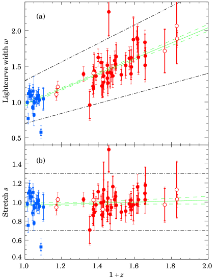
Figure 3: (a) The observed light-curve width factor $w$ vs $1+z$. The blue squares correspond to the Calán/Tololo SNe, the solid red circles are for the subset of 35 SCP SNe used in this paper. The open red circles are for the remainder of the 42 SCP fully-analyzed SNe. The band delineated by the black dash dotted lines corresponds to stretch values 0.7 to 1.3 which encompass the bulk of the data, except for two outliers. The green line is the best linear fit to the data as discussed in the text. The band delineated by the two green dashed curves correspond to the $\pm 1\sigma$ values. (b) The stretch $s$ vs $1+z$. Stretch is defined as the observed light-curve width $w$ divided by $1+z$ for each SN. The points and lines are defined as in (a).

Light curve width factor $w$ and stretch factor $s$ versus $1+z$ are shown in Figure 3(a) and Figure 3(b) respectively for the Calán/Tololo and SCP SNe. We are interested in the possible variation of $w$ and $s$ with $z$. We test for the $z$ dependence of these distributions by fitting straight lines to the data. If the SNe in the distant past were different, i.e. due to evolution effects, the distribution might show a slope $ds/dz$. The fits described below were carried out for the entire 18 Calán/Tololo SNe together with 40 of the SCP SNe. Two SCP SNe, SN1992bi and SN1992br, have stretch factors outside the range $0.7<s<1.3$, and are excluded from the fits as outliers representing non-Gaussian tails to the distributions or aberrant objects. As discussed in P99, these will not be important for the present analysis.

In performing the fit of the function $s=a+b\,z$ to the data shown in Figures 3(b) the total uncertainty for each point is $\sigma_{s^{\prime}}=\sqrt{\sigma_{s}^{2}+\delta_{s}^{2}}$ where $\delta_{s}^{2}$ is the intrinsic stretch dispersion and $\sigma_{s}$ from Tables 1 and 2 is from the individual light-curve fit uncertainty. We estimate this intrinsic dispersion by requiring that the reduced $\chi^{2}$ is near unity. This yields an rms deviation $\delta_{s}\approx 0.08$. The intrinsic width $\delta_{s}$ of the stretch factor distribution can also be obtained from a Gaussian fit to Figure 4 in P99. This gives a consistent value for $\delta_{s}$ of $\sim 0.1$. The errors used in the fit to the $w$ distribution shown in Figures 3(a) are treated similarly. In Figure 3 (a) and (b) both errors $\sigma_{s}$ and $\sigma_{s^{\prime}}$ are shown on the error bars.

We find that our data is consistent with $1+z$ lightcurve broadening and a redshift independent SN stretch distribution. Fits to Figure 3 (a) and (b) yield different information. The linear fit shown in Figure 3(a) has $dw/dz=1.07\pm 0.06$. If there were no $z$ dependence in $w$ this slope would be $0$, here assuming no evolutionary change in $s$. Hence the evidence for the presence of a $1+z$ factor is $1.07/0.06\approx 18$ standard deviations. Figure 3(b) shows a slope $ds/dz=0.05\pm 0.05$. The extent by which this slope differs from $0$ measures the possible evolution effects on $s$, here assuming a $1+z$ dependence of $w$. The result indicates that $ds/dz<0.09$ at the $95\%$ confidence level out to $z\sim 0.8$. We obtain essentially the same results from fits in which the 2 outliers are included (for a total of 60 SNe), and when the 35 rather than the 42 SCP SNe, less 2 outliers, are used (for a total of 51 SNe). Note that this analysis does not account for sample selection effects — such as possible preferred discovery of high stretch SNe near the flux limit of each SNe search — which may need to be accounted for in future datasets.

When we compare this result to the alternate theories, it is clear that they are severely challenged or simply ruled out. The tired light theories (Zwicky (1929); Hubble & Tolman (1935); Hubble (1936); Marič et al. (1977); Chow (1977); La Violette (1986) would not yield this slowing of the light curves, and thus do not fit this dataset. Variable mass theories (Narlikar (1977); Narlikar & Arp (1993, 1997) would apparently require a series of coincidences: the radioactive decay times, the timescales for the radiative transport processes in the SN atmosphere, and the atomic transitions would all have to vary as $(1+z)$ due to variations in the masses of elementary particles for the theory to account for the data. All these effects would have to result in making the observed spectra similar.

5 Discussion

We have shown that a single stretch factor varying the timescale of the SNe Ia accounts very well for the restframe $B$ band light curve both before and after maximum light (up to 40 days past maximum). It is not understood from the current state of the theory of SNe Ia whether this is a fortuitous coincidence or a reflection of some physics timescale (Höflich, 1995; Höflich & Khokhlov, 1996; Nugent, 1997; Pinto & Eastman, 2000; Arnett, 2000; Hillebrandt & Niemeyer, 2000). Although we do not necessarily expect this single timescale stretch factor to hold for all wavelength bands, we do have evidence that it applies in the $V$ band and (with less confidence) the $U$ band. We will analyze these results in future work.

The current analysis does not address the relationship between the SN Ia light curve stretch and its peak luminosity. This requires another analysis that will be presented elsewhere. However, it is important to note that the current $B$ band template stretched by a factor $s$ fits the data as well as any parameterization can, given the current data sets. It will therefore yield a peak-luminosity correlation with as small a dispersion as can be obtained by any other B-band light-curve parameterization.

The comparison of the low-redshift and high-redshift composite supernovae light curves in Figure 2 provide a first-order test for evolution of supernovae as we go back to the $z\sim 0.5$ epoch. The close match of the light curves is suggestive that little evolution has occurred.

A recent analysis of low-redshift early light curves by Riess et al (1999a, 1999b) suggested that the explosion date of the low-redshift SNe Ia was earlier than that of the high-redshift SNe. The analyses of our early light curve uncertainty in Section 6 and in AKN2000 show that the difference between the two data sets is not very significant at this stage, less than $\sim$2$\sigma$. This will be an interesting region of the light curve to pursue with future data, particularly over a range of host galaxy environments that would be expected to show variations in metallicity and progenitor ages. We are currently working with the supernova research community on generating a much more extensive low-redshift dataset to study this question. However, it is important to remember that – as pointed out by AKN2000 – the template differences have a negligible influence on the corrected peak magnitudes of the P99 SNe, and thus the cosmological parameters derived therein are unchanged.

Finally, it is interesting to note that while the redshift of the light measures the expansion of the universe with a “microscopic clock” of period, typically $T=2\times 10^{-15}$ seconds, our “macroscopic clocks”, the Type Ia SNe, measure the expansion over a $\approx 4$ week period or $T\approx 2.4\times 10^{6}$ seconds. The $1+z$ expansion effect is thus consistent for two time periods which differ by 21 orders of magnitude.

6 Acknowledgments

The observations described in this paper were primarily obtained as visiting/guest astronomers at the Cerro Tololo Inter-American Observatory 4-meter telescope, operated by the National Optical Astronomy Observatory under contract to the National Science Foundation; the Keck I and II 10-m telescopes of the California Association for Research in Astronomy; the Wisconsin-Indiana-Yale-NOAO (WIYN) telescope; the European Southern Observatory 3.6-meter telescope; the Isaac Newton and William Herschel Telescopes, operated by the Royal Greenwich Observatory at the Spanish Observatorio del Roque de los Muchachos of the Instituto de Astrofisica de Canarias; the Hubble Space Telescope, and the Nordic Optical 2.5-meter telescope. We thank the dedicated staff of these observatories for their excellent assistance in pursuit of this project. In particular, Dianne Harmer, Paul Smith and Daryl Willmarth were extraordinarily helpful as the WIYN queue observers. We thank Gary Bernstein and Tony Tyson for developing and supporting the Big Throughput Camera at the CTIO 4-meter; this wide-field camera was important in the discovery of many of the high-redshift supernovae. This work was supported in part by the Physics Division, E. O. Lawrence Berkeley National Laboratory of the U. S. Department of Energy under Contract No. DE-AC03-76SF000098, and by the National Science Foundation’s Center for Particle Astrophysics, University of California, Berkeley under grant No. ADT-88909616. Support for this work was provided by NASA through grant number HST-GO-07336 from the Space Telescope Science Institute, which is operated by AURA, Inc., under NASA contract NAS5-26555. A. G. acknowledges the support of the Swedish Natural Science Research Council. The France-Berkeley Fund and the Stockholm-Berkeley Fund provided additional collaboration support.

Table 2. Fit parameters for the Calán/Tololo data

 Name $z$ $w$ $\sigma_{w}$ $s$ $\sigma_{s}$ $\chi^{2}/DoF$  1990O 0.030 1.09 0.03 1.06 0.03 1.53  1990af 0.050 0.82 0.02 0.78 0.02 0.51  1992P 0.026 1.15 0.08 1.12 0.08 1.45  1992ae 0.075 1.09 0.09 1.02 0.08 0.78  1992ag 0.026 1.14 0.04 1.11 0.04 2.15  1992al 0.014 0.99 0.02 0.98 0.02 1.71  1992aq 0.101 1.04 0.14 0.95 0.13 0.65  1992bc 0.020 1.12 0.01 1.09 0.01 3.14  1992bg 0.036 1.09 0.05 1.05 0.05 1.68  1992bh 0.045 1.15 0.05 1.10 0.05 3.77  1992bl 0.043 0.92 0.03 0.88 0.03 2.15  1992bo 0.018 0.77 0.01 0.76 0.01 1.29  1992bp 0.079 1.03 0.03 0.95 0.03 1.35  1992br 0.088 0.58 0.04 0.53 0.04 1.39  1992bs 0.063 1.05 0.05 0.99 0.05 1.43  1993B 0.071 1.06 0.09 0.99 0.08 1.14  1993O 0.052 0.99 0.01 0.94 0.01 1.26  1993ag 0.050 1.01 0.04 0.96 0.04 1.16

Table 3. $B$ templates, in Normalized Flux, used by the Supernova Cosmology Project

The headers: “SCP1997” refers to Leibundgut (1988) from day -5 on up, with a linear extension (in magnitude) to earlier times shown in flux here. As discussed in the text, this is the template used in Perlmutter et al. (1997, 1999). Tables 1, 2 and 7 as well as Figure 2(e), are based on this template. “Parab - 18” uses a parabolic turn-on at $-17.6$ days from a fit to the 35 SCP SNe. Tables 4 and 6 and Figures 1 and 2, except 2(c) and 2(e), are based on this template. “Parab -20” uses the parabolic turn-on at -20 days following the early rise-time data of Riess et al. (1999a). Table 5 and Figure 2(c) are based on this template. After -10 days the two parabolic templates coincide.  SCP1997   Parab   Parab  Day -18 -20  -25 0.001 0.000 0.000  -24 0.001 0.000 0.000  -23 0.002 0.000 0.000  -22 0.003 0.000 0.000  -21 0.005 0.000 0.000  -20 0.007 0.000 0.000  -19 0.012 0.000 0.005  -18 0.019 0.000 0.019  -17 0.030 0.005 0.044  -16 0.048 0.025 0.080  -15 0.076 0.063 0.127  -14 0.120 0.118 0.183  -13 0.189 0.190 0.248  -12 0.277 0.279 0.324  -11 0.388 0.385 0.410  -10 0.494 0.508 0.508  -9 0.597 0.622  -8 0.674 0.714  -7 0.746 0.789  -6 0.810 0.849  -5 0.868 0.896  -4 0.915 0.933  -3 0.952 0.961  -2 0.979 0.982  -1 0.995 0.995  0 1.000 1.000  1 0.995 0.995  2 0.979 0.978  3 0.953 0.950  4 0.918 0.910  5 0.875 0.863  6 0.827 0.811  7 0.773 0.759  8 0.718 0.707  9 0.661 0.656  10 0.604 0.606  11 0.550 0.558  12 0.498 0.511  SCP1997   Parab  $-$Day -18   & -20  $-$13 0.449 0.466  $-$14 0.404 0.423  $-$15 0.363 0.381  $-$16 0.327 0.342  $-$17 0.293 0.306  $-$18 0.264 0.272  $-$19 0.238 0.241  $-$20 0.215 0.215  $-$21 0.195 0.192  $-$22 0.178 0.172  $-$23 0.162 0.155  $-$24 0.149 0.142  $-$25 0.137 0.130  $-$26 0.127 0.120  $-$27 0.118 0.112  $-$28 0.110 0.105  $-$29 0.103 0.099  $-$30 0.097 0.094  $-$31 0.092 0.090  $-$32 0.087 0.087  $-$33 0.083 0.084  $-$34 0.080 0.081  $-$35 0.076 0.078  $-$36 0.074 0.076  $-$37 0.071 0.073  $-$38 0.069 0.071  $-$39 0.067 0.069  $-$40 0.065 0.067  $-$41 0.064 0.065  $-$42 0.062 0.064  $-$43 0.061 0.062  $-$44 0.060 0.060  $-$45 0.059 0.059  $-$46 0.058 0.058  $-$47 0.057 0.057  $-$48 0.056 0.056  $-$49 0.055 0.055  $-$50 0.054 0.054

Table 4. $\chi^{2}$ Fits of the SCP Data to the

Composite Parabolic Template “Parab-18”

Corresponding to $t_{exp}=-17.6$ Days

Columns 1 and 2 define the Epoch Interval,

Columns 3 and 4 give the $\chi^{2}$ and

$\chi^{2}$ per Degree of Freedom. See Fig 2 (b)

Epoch $\chi^{2}$ $\chi^{2}/$DoF Start End  -25 -20 27.8 1.16  -20 -15 23.7 0.99  -15 -10 35.8 0.58  -10 -5 72.4 0.95  -5 0 101.7 1.02  0 5 111.6 0.88  5 10 74.5 0.89  10 15 62.2 0.91  15 20 25.6 0.47  20 25 83.3 0.95  25 30 70.1 1.02  30 35 49.1 0.88  35 40 25.8 1.51  -25 40 763.5 0.905

Table 5. $\chi^{2}$ Fits of the SCP Data to the

Composite Parabolic Template “Parab-20”

Corresponding to $t_{exp}=-20$ Days

Column headings as in Table 4. See Figure 2(d)

Epoch $\chi^{2}$ $\chi^{2}/$DoF Start End  -25 -20 29.3 1.01  -20 -15 27.5 0.65  -15 -10 28.4 0.71  -10 -5 71.2 0.94  -5 0 105.0 1.00  0 5 115.6 0.92  5 10 70.1 0.86  10 15 63.6 0.96  15 20 26.1 0.49  20 25 84.6 0.95  25 30 67.9 1.03  30 35 52.0 0.91  35 40 21.4 1.34  -25 40 762.6 0.906

Table 6. $\chi^{2}$ Fits of the Calán/Tololo data

to the Composite Parabolic Template^∗

Column headings as in Table 4. See Figure 2(c)

Epoch $\chi^{2}$ $\chi^{2}/$DoF Start End  -10 -5 25.3 1.95  -5 0 39.7 2.09  0 5 17.1 0.47  5 10 59.5 1.06  10 15 55.7 1.39  15 20 28.9 1.25  20 25 14.8 0.93  25 30 11.2 0.62  30 35 21.1 1.32  35 40 17.0 0.81  -10 40 290.3 1.143 * In this Table some of the photometry errors were extremely small. We used a minimum error of 0.007, in normalized units, here.

Table 7. $\chi^{2}$ Fits of the SCP Data to the

Composite Exponential Template “SCP1997”

the Extended Leibundgut Template

Column headings as in Table 4. See Figure 2(e)

Epoch $\chi^{2}$ $\chi^{2}/$DoF Start End  -25 -20 27.5 1.15  -20 -15 24.3 1.01  -15 -10 36.8 0.59  -10 -5 105.2 1.38  -5 0 105.7 1.06  0 5 110.8 0.87  5 10 75.3 0.90  10 15 73.4 1.08  15 20 29.3 0.54  20 25 83.8 0.95  25 30 69.1 1.00  30 35 49.2 0.88  35 40 25.4 1.49  -25 40 815.7 0.966

Table 8. $\chi^{2}$ Fits of the SCP Data to the

Parabolic Template “Parab-18”

with only $1+z$ but not $s$ factored out

This Table illustrates the effect of the

factor $s$ both before and after Maximum light.

Column headings as in Table 4.

Epoch $\chi^{2}$ $\chi^{2}/$DoF Start End  -25 -20 24.2 1.86  -20 -15 30.3 1.08  -15 -10 231.8 4.55  -10 -5 250.2 3.05  -5 0 104.3 1.03  0 5 112.4 0.89  5 10 125.6 1.38  10 15 57.9 0.95  15 20 110.1 1.84  20 25 98.6 1.15  25 30 105.0 1.36  30 35 45.9 1.12  35 40 35.4 1.18  -25 40 1330.7 1.582

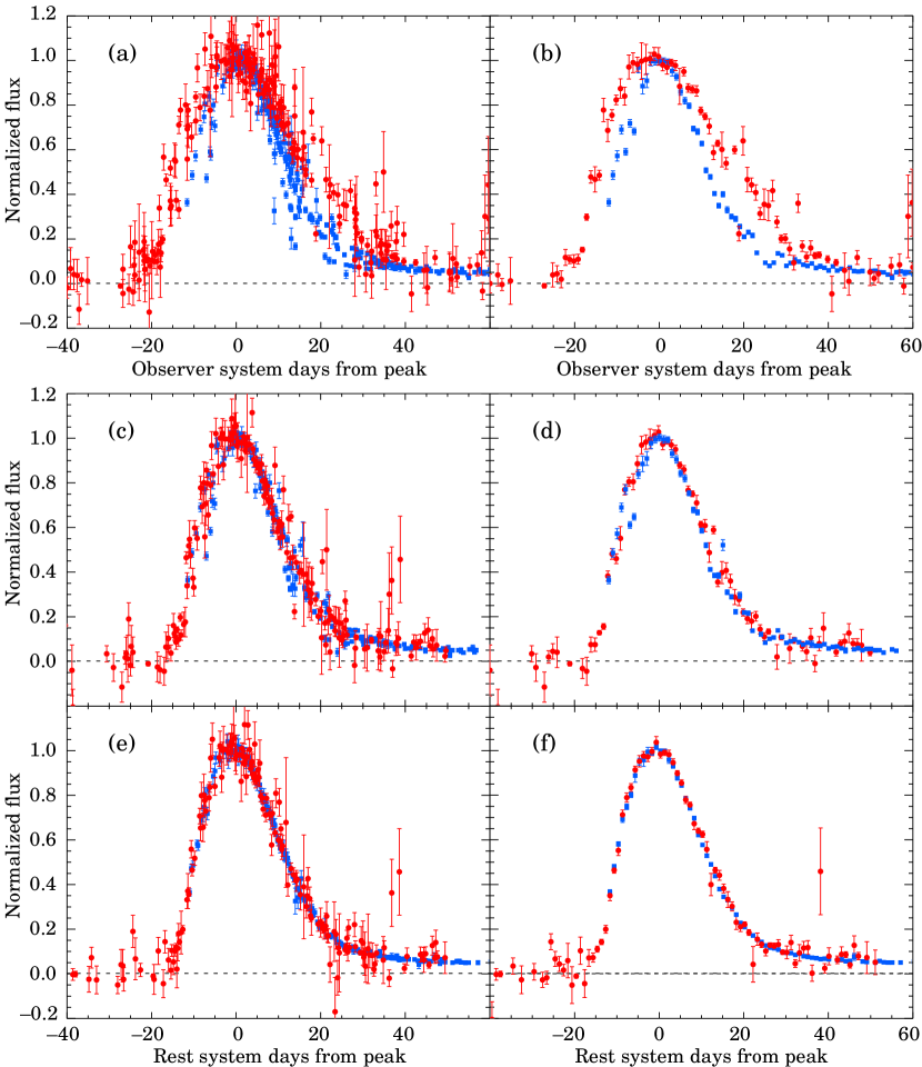
Figure 1: (a) The photometry points for the 35 SCP (full red circles) and 18 Calán/Tololo SNe (blue squares), fitted to Parab-18 with the maximum flux normalized to unity and the time of maximum adjusted to zero in the observer system. (b) shows the same data as in (a) averaged over one-day intervals and over each set of SNe. (c) and (d) show the same data, transformed to the rest system. In (e) and (f) the time axis for each photometry point is additionally divided by the corresponding stretch factor $s$.

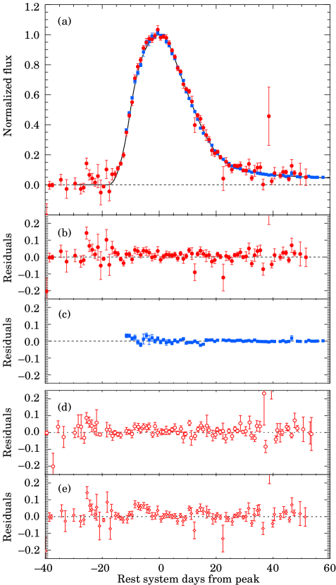
Figure 2: (a) The same distribution as in Figure 1(f) with the SNe in the two data sets fitted to Parab-18. The template curve for Parab-18 is shown in black. (b) Residuals for the SCP (solid red circles) photometry fits to Parab-18. Here the epoch between -40 and -20 days has no SN signal, the data comes from the reference images which have shorter exposures and hence larger errors (see Table 4). (c) Residuals for the Calán/Tololo (blue squares) photometry fits to Parab-18 (see Table 6 ). (d) The open red circles show the residuals for the SCP data from the fit to Parab-20 (template not shown), where the early rise is based on the data of Riess et al. (1999a). See Table 5. (e) Residuals for the SCP data (open red diamonds) fitted to the template SCP1997 (template not shown). Note that the “bumps” near -5 days and 15 days (see also Table 7) were eliminated for the templates Parab-18 and Parab-20.

References

- Aldering , Knop & Nugent (1999) Aldering, G., Knop R. & Nugent P. 2000, AJ, 119, 2110
- Arnett (2000) Arnett, W. D. 1999, astro-ph/990903
- Arp (1987) Arp, H.C. 1987, Quasars, Redshifts and Controversies (Interstellar Media, Berkeley)
- Arp et al. (1990) Arp, H.C., Burbidge, G., Hoyle, F., Narkikar, J. V., & Wickramasinghe, N. C. 1990, Nature, 346, 807
- Arp et al. (1994) Arp, H.C., et al. 1994, ApJ, 430, 74
- Chow (1977) Chow, T. L. 1981, Lett. Nuovo Cimento, 32, 351
- Goldhaber et al. (1995) Goldhaber, G., et al. 1995, in Presentations at the NATO ASI in Aiguablava, Spain, LBL-38400, page III.1; also published in Thermonuclear Supernova, P. Ruiz-Lapuente, R. Canal, and J.Isern, editors, Dordrecht: Kluwer, page 777 (1997)
- Goldhaber (1998a) Goldhaber, G. 1998a, XXVI SLAC Summer Institute ”Gravity: From the Hubble Length to the Plank Length” Aug 1998
- Goldhaber (1998b) Goldhaber, G. 1998b, B.A.A.S., 193, 47.13
- Groom (1998) Groom, D. E. 1998, B.A.A.S., 193, 111.02
- Hamuy et al. (1995) Hamuy, M., Phillips, M. M., Maza, J., Suntzeff, N. B., Schommer, R. A., & Aviles, R. 1995, AJ, 109, 1
- Hamuy et al. (1996) Hamuy, M., Phillips, M. M., Maza, J., Suntzeff, N. B., Schommer, R. A., & Aviles, R. 1996, AJ, 112, 2391
- Hillebrandt & Niemeyer (2000) Hillebrandt W., & Niemeyer J. C., 2000, A R A & A in press (astro-ph/0006305)
- Höflich (1995) Höflich, P. 1995, ApJ, 443, 89
- Höflich & Khokhlov (1996) Höflich, P., & Khokhlov, A. M. 1996, ApJ, 457, 500
- Hoyle & Fowler (1960) Hoyle, F., & Fowler, W. A. 1960, ApJ, 132, 565
- Hubble & Tolman (1935) Hubble, E., and Tolman, R. C. 1935, ApJ, 82, 302
- Hubble (1936) Hubble, E. 1936, ApJ, 84, 517
- James & Roos (1994) James, F., & Roos, M., “MINUIT, Function Minimization and Error Analysis,” CERN D506 (Long Writeup). Available from the CERN Program Library Office, CERN-IT Division, CERN, CH-1211, Geneva 21, Switzerland
- Kim, Goobar, & Perlmutter (1996) Kim, A., Goobar, A., & Perlmutter, S. 1996, PASP, 108, 190
- Lee et al. (2000) Lee, A., Bloom E. D. & Petrosian V. 2000, astro-ph/0002218
- Leibundgut (1988) Leibundgut, B., 1988, Ph. D. Thesis, Univesity of Basel
- Leibundgut et al. (1991) Leibundgut, B., et al. 1991, ApJ, 371, L23
- Leibundgut et al. (1991) Leibundgut, B., Tammann, G. A., Cadonau, R., & Cerrito, D. 1991, Astron. Astrophys. Suppl. Ser., 89, 537
- Leibundgut et al. (1996) Leibundgut, B., et al. 1996, ApJ, 466, L21
- Lentz et al. (2000) Lentz, E. J., Baron, E., Branch, D. , Hauschildt, P. H., & Nugent, P. E. 2000, ApJ., 530, 966
- Lira et al. (1998) Lira, P., et al. AJ, 115, 234
- Marič et al. (1977) Marič, Z., Moles, M., and Vigier, J. P. 1977, Lett. Nuovo Cimento, 18, 269
- Metzger et al. (1997) Metzger, M. R., et al. 1997, Nature 387, 876
- Narlikar (1977) Narlikar, J. V. 1977, Ann. Phys., 107, 325
- Narlikar & Arp (1993) Narlikar, J. V., & Arp, H.C. 1993, ApJ., 405, 51
- Narlikar & Arp (1997) Narlikar, J. V., & Arp, H.C. 1993, ApJ, 482, L119
- Norris et al. (1995) Norris J. P., et al. 1995, ApJ, 439, 542
- Nugent (1997) Nugent, P., 1997, Ph. D. Thesis, University of Oklahoma, Ch. 4
- Nugent et al. (1997a) Nugent, P., Baron E., Branch D., Fisher A. & Hauschildt P. 1997a, ApJ., 485, 812
- Nugent, Kim & Perlmutter (2001) Nugent, P., Kim, A. G. & Perlmutter, S., 2001, PASP, submitted
- Perlmutter et al. (1995) Perlmutter, S., et al. 1995, in Presentations at the NATO ASI in Aiguablava, Spain, LBL-38400, page I.1; also published in Thermonuclear Supernova, P. Ruiz-Lapuente, R. Canal, and J.Isern, editors, Dordrecht: Kluwer, page 749 (1997)
- Perlmutter et al. (1997) Perlmutter, S., et al. 1997, ApJ, 483, 565
- Perlmutter et al. (1999) Perlmutter, S., et al., ApJ, 517, 565
- Phillips (1993) Phillips, M. M., ApJ Lett., 413, L105
- Pinto & Eastman (2000) Pinto P. A. & Eastman R. G. 2000, ApJ, 530, 744
- Piran (1992) Piran T. 1992, ApJ Lett. 389, L45
- Pskovskii (1977) Pskovskii, Y.P. 1977, Soviet Astron., 21, 675
- Pskovskii (1984) Pskovskii, Y.P. 1984, Soviet Astron., 28, 658
- Riess, Press, & Kirshner (1995) Riess, A. G., Press, W. H., & Kirshner, R. P. 1995, ApJ, 438, L17
- Riess, Press, & Kirshner (1996) Riess, A. G., Press, W. H., & Kirshner, R. P. 1996, ApJ, 473, 88
- Riess et al. (1997) Riess, A., et al. 1997a, AJ, 114, 722
- Riess et al. (1998) Riess, A., et al. 1998, AJ, 116, 1009
- Riess et al. (1999) Riess, A., et al. 1999, AJ, 117, 707
- Riess et al. (1999a) Riess, A., et al. 1999a, AJ, 118, 2675
- Riess et al. (1999b) Riess, A., et al. 1999b, AJ, 118, 2668
- Rust (1974) Rust, B. W., 1974 Ph. D. Thesis, University of Illinois; ORNL Report 4953
- Sandage & Perelmutter (1991) Sandage, A & Perelmutter, J. M. 1991, ApJ, 370, 455
- Suntzeff et al. (1999) Suntzeff, N. B., 1999, AJ, 117, 1175
- La Violette (1986) La Violette, P. A. 1986, ApJ, 301, 544
- Weinberg (1972) Weinberg, Steven, Gravitation and Cosmology: Principles and Applications of the General Theory of Relativity, (New York: John Wiley & Sons), p. 30
- Wilson (1939) Wilson, O. C. 1939, ApJ, 90, 634
- Zwicky (1929) Zwicky, F. 1929, Proc. Nat. Acad. Sci., 15, 773
Table 1. Fit parameters for 42 Type 1a Supernovae reported by the Supernova Cosmology Project (Perlmutter et al. (1999)). For the present analysis we require good -band photometry and corrections to , so the 7 objects with qualifying comments are not used.
Name Comments 1992bi 0.458 2.26 0.34 1.55 0.23 0.91 1994F 0.354 0.96 0.19 0.71 0.14 1.74 1994G 0.425 1.32 0.24 0.92 0.17 0.71 Late 1994H 0.374 1.19 0.07 0.87 0.05 1.59 1994al 0.420 1.22 0.13 0.86 0.09 0.94 1994am 0.372 1.22 0.05 0.89 0.04 1.73 1994an 0.378 1.44 0.23 1.04 0.17 1.38 1995aq 0.453 1.27 0.15 0.87 0.10 1.21 1995ar 0.465 1.42 0.21 0.97 0.14 2.06 1995as 0.498 1.64 0.16 1.09 0.11 0.57 1995at 0.655 1.84 0.12 1.11 0.07 0.80 1995aw 0.400 1.62 0.06 1.16 0.04 1.80 1995ax 0.615 1.88 0.18 1.16 0.11 1.17 1995ay 0.480 1.36 0.12 0.92 0.08 1.07 1995az 0.450 1.41 0.10 0.97 0.07 0.63 1995ba 0.388 1.36 0.06 0.98 0.04 1.13 1996cf 0.570 1.61 0.11 1.03 0.07 1.06 1996cg 0.490 1.58 0.07 1.06 0.05 0.85 1996ci 0.495 1.53 0.07 1.02 0.05 1.21 1996ck 0.656 1.51 0.20 0.91 0.12 1.06 1996cl 0.828 2.07 0.53 1.13 0.29 1.12 band 1996cm 0.450 1.33 0.09 0.92 0.06 0.80 1996cn 0.430 1.28 0.10 0.89 0.07 1.30 1997F 0.580 1.62 0.11 1.02 0.07 0.86 1997G 0.763 1.71 0.30 0.97 0.17 1.17 band 1997H 0.526 1.38 0.08 0.90 0.05 0.86 1997I 0.172 1.11 0.04 0.94 0.03 5.60∗∗ band 1997J 0.619 1.63 0.21 1.00 0.13 0.94 1997K 0.592 1.87 0.30 1.18 0.19 0.62 1997L 0.550 1.51 0.14 0.98 0.09 2.57 1997N 0.180 1.21 0.02 1.03 0.02 1.72 band 1997O 0.374 1.40 0.10 1.02 0.07 0.75 Outlier 1997P 0.472 1.40 0.06 0.95 0.04 1.30 1997Q 0.430 1.36 0.04 0.95 0.03 1.09 1997R 0.657 1.65 0.12 0.99 0.07 1.06 1997S 0.612 1.90 0.10 1.18 0.06 1.66 1997ac 0.320 1.39 0.03 1.05 0.02 0.79 1997af 0.579 1.39 0.08 0.88 0.05 0.95 1997ai 0.450 1.52 0.20 1.04 0.14 0.82 1997aj 0.581 1.49 0.09 0.94 0.06 1.75 1997am 0.416 1.55 0.07 1.10 0.05 1.24 1997ap 0.830 1.88 0.09 1.03 0.05 1.04 band * No -band data before 14 days; primary photometry from band. ** Here the V template was used while a template between V and R would be more appropriate. A fit to Parab-18 gives .