Fine-Tuning Solution for Hybrid Inflation in Dissipative Chaotic Dynamics

Abstract

We study the presence of chaotic behavior in phase space in the pre-inflationary stage of hybrid inflation models. This is closely related to the problem of initial conditions associated to these inflationary type of models. We then show how an expected dissipative dynamics of fields just before the onset of inflation can solve or ease considerably the problem of initial conditions, driving naturally the system towards inflation. The chaotic behavior of the corresponding dynamical system is studied by the computation of the fractal dimension of the boundary, in phase space, separating inflationary from non-inflationary trajectories. The fractal dimension for this boundary is determined as a function of the dissipation coefficients appearing in the effective equations of motion for the fields.

PACS number(s): 98.80 Cq

In press Physical Review D

I Introduction

Among the various proposed models for implementing inflation, the hybrid inflation model [1] is one of the most attractive ones due to the possibility of its implementation in the context of supersymmetry and supergravity models [2]. The principle behind these models for inflation are basically based on models where the inflaton is coupled to one or more scalar fields. The inflationary phase is characterized by an initial phase in the evolution of the fields where the inflaton field slowly moves towards zero vacuum expectation value, till it approaches a critical value which then induces a spontaneous symmetry breaking in one of the other fields which are coupled to the inflaton, after which the fields quickly evolve to their vacuum states and inflation ends.

It has been shown in the context of supergravity motivated models [3] that for inflaton field amplitudes larger than the Planck mass there will appear large quantum corrections in the inflaton’s effective potential, destroying the flatness of the inflaton’s potential as required by the slow-roll conditions for inflation. The question then turns to whether inflation can be achieved in these models for initial inflaton field amplitudes smaller than the Planck scale, where a reliable model could be constructed. But in this case it has been shown [4] that small fluctuations of the other fields coupled to the inflaton are efficiently able to prevent the onset of inflation, or quickly drive previous inflationary trajectories to non-inflationary trajectories and therefore making inflation to end before enough e-folds of inflation have been produced ($N_{e}\gtrsim 70$ as required) to solve the usual cosmological horizon and flatness problems. This is related to the homogeneity requirement over Hubble size distances [5] in order to inflation to begin. In the context of hybrid inflation this problem is even more severe, requiring an extreme fine-tuning of the initial conditions in order to have sufficient homogeneity, with negligible spatial and time derivatives of the other fields that are coupled to the inflaton, over regions extending far beyond a few Hubble lengths.

A few solutions to this homogeneity, or fine-tuning problem, have been proposed. The authors in Ref. [6] for example propose two-stage inflation models where a first short inflationary phase would smooth a large enough region in phase space making then possible a later longer second inflationary phase. In Ref. [7] it is analyzed the possibility of the solution of the fine-tuning problem in the context of more complicate generalizations of the hybrid inflation model as motivated from higher-dimensional scalar field models or brane cosmology.

Here I will be interested in investigating the possible role of how effective field interactions may shed further light in this fine-tuning problem in the pre-inflationary phase. This is mostly motivated from several works on the effective dynamics of scalar field configurations, which have shown that dissipation is intrinsically present in the field dynamics [8, 9, 10, 11, 12, 13, 14, 15]. In special, the role of dissipation in all of these works has been emphasized. We can trace the origin of these effects by considering the dynamics of a given system, which interacts with a sufficiently large environment (in the sense of degrees of freedom). One well known example of this, in the context of statistical mechanics, is the model of an oscillator, taken as being the system, in interaction with a large number of harmonic oscillators which are taken as representing the environment. By functionally integrating over the environment degrees of freedom we can then show that the dynamics of the system oscillator will be dissipative, with an equation of motion of the form of a Langevin-like one [16, 14].

The dynamic of interacting fields has being a subject of intense study, in both Minkowski space-time [8, 10, 15], as also in FRW space-times [11, 12], with special interest in studying the dynamics of the inflaton field both during and immediately after the inflationary phase. In particular, in Refs. [17, 18] it was shown the importance of considering dissipative effects (due to inflaton’s decay) during inflation. The authors in [17] have shown how dissipation can influence the usual scenario of inflation, as also the effect of dissipation on the field trajectories in phase space. Strong dissipative regimes for field evolution have in special motivated the implementation of new inflationary models called “warm inflation” [19]. The viability of the construction of microscopic motivated models of strong dissipative inflaton models has been shown possible in the context of superstring inspired models in Ref. [20] and argued also possible for more general models in [21].

On very general grounds, we are then lead to inquire about the possible role of field dissipation also at the early stages of inflation and in special to its role in smoothing large regions in phase space and thus easing considerable the homogeneity requirements for the onset of inflation and, consequently, providing a natural solution for the problem of fine-tuning associated to hybrid inflation. It is easy to understand the effect of dissipation on the initial conditions problem. For the regime of initial inflaton amplitude below the Planck scale the energy density is small at the beginning of inflation, resulting in a small Hubble parameter $H$, which determines how fast the inflaton energy is converted to expansion. For small values of $H$ the coupling of the fields to the background metric of gravity is small and the corresponding friction like term in the equations of motion, of the form $3H\dot{\phi}$, is small. This results in a very long evolution for the fields, where those fields coupled to the inflaton oscillate around zero several times, generating strong sensitivity to very small variations of the initial conditions and resulting in a complete indetermination of the final outcome of the fields’ trajectories, which can be evolution toward an inflationary regime or to the minima of the potential. The behavior of the fields’ trajectories in the early times before a required long inflationary regime is then extremally chaotic. In the language of dynamical systems we have two types of attractors in the system, represented by the inflationary regime and the minima of the potential. The presence of dissipation works in damping the fluctuations of the fields in this initial critical time, suppressing the chaotic motions, which we then expect, from the results of Ref. [17], will bias the inflaton field trajectory toward the inflationary one. In fact, recently a study done by the authors in Ref. [22] have indicated that additional damping terms in the inflaton equation of motion could alleviate many of the problems related to the homogeneity requirements before inflation. Another study done by the authors in Ref. [23], using a supersymmetric hybrid inflation model, have also indicated that particle production may be a way to relax the extreme homogeneity requirements for hybrid inflation.

Here we will then be mostly concerned in determining for what magnitude of dissipation will the outcome of the evolution of the fields tend mostly toward the inflationary regime, or in the dynamical system approach, determine how fast dissipation will change the chaotic regime, characterized by unstable inflationary trajectories, to a non-chaotic one, with stable inflationary trajectories. We study chaos in our dynamical system of equations by means of the measure of the fractal dimension (or dimension information) [for a review and definitions, see e.g., Ref. [24]], which gives a topological measure of chaos for different space-time settings and it is a quantity invariant under coordinate transformations, providing then an unambiguous signal for chaos in cosmology and general relativity problems in general [25, 26]. The method we apply in this work for quantifying chaos is then particularly useful in this cosmological pre-inflationary scenario context we are studying, in which case other methods may be ambiguous, like, for example, the determination of Lyapunov exponents, which does not give a coordinate invariant measure for chaos, as discussed in [25, 26]. Also, other methods for studying chaotic systems, like for example by Poincaré sections, are not suitable in the case we are interested here, in which case chaos is mostly a transitory phenomenon (it ends by the time the fields reach the potential minima, or when the inflaton enters the inflationary region). By computing the fractal dimension characterizing this chaotic behavior, which is related to the uncertainty in the system parameter values to predict the final outcome from a given initial condition (we may say that the boundaries of initial conditions that lead to inflation or evolution towards the potential minima are mixed) we are then able to infer the naturalness of inflation for different settings of the initial conditions. To our knowledge, this is the first time that this kind of study is performed in the context of a dissipative dynamical system in cosmology and applied to the initial condition problem of inflation in particular.

The paper is organized as follows: in Sec. II I give the basic equations defining the dynamical system and I discuss some of their properties. In Sec. III I present the numerical analysis of the dynamical system and the computation of the fractal dimension as a function of the magnitude of dissipation. From this analysis one will be able to conclude about the general effect of dissipation in the evolution of the fields and how it works in favor of the inflationary regime. Finally in Sec. IV I give the concluding remarks.

II The Model and Its Properties

The model I will study here consists of the simplest hybrid inflation model, with a scalar field $\phi$ (the inflaton) coupled to another scalar field $\sigma$, which triggers the end of inflation. The potential is [1]

$$V(\phi,\sigma)=\frac{\lambda}{4}(\sigma^{2}-M^{2})^{2}+\frac{m^{2}}{2}\phi^{2}+\frac{g^{2}}{2}\phi^{2}\sigma^{2}\;,$$ (1)

where the parameters $M^{2},\;m^{2}$ and the couplings $\lambda$ and $g^{2}$ are positive. In the following I will treat only the case of homogeneous fields, $\phi\equiv\phi(t)$ and $\sigma\equiv\sigma(t)$, which is the usual case in the works dealing with the initial condition problem in hybrid inflation. The interpretation of inflation from the potential (1) is the standard one. For values of $\phi$ larger than a critical value $\phi_{\rm cr}$, where $\phi^{2}_{\rm cr}=\lambda M^{2}/g^{2}$, there is no symmetry breaking in the $\sigma$-field direction and $\sigma=0$ is a local minimum of the potential. We are interested in the region where $M_{\rm pl}^{2}\gg\phi^{2}\gtrsim\phi^{2}_{\rm cr}$ where inflation takes place (the false vacuum dominated regime). After the inflaton field drops below $\phi_{\rm cr}$, symmetry breaking occurs in the $\sigma$ field direction of the potential. At this point the fields quickly move towards the minima $\sigma=\pm M$, $\phi=0$ and inflation ends.

The chaotic properties of the classical (homogeneous) equations of motion, in Minkowski spacetime, for a model with potential similar to the one given by Eq. (1) were studied in Ref. [27], while the full effective equations of motion in Minkowski spacetime were studied by Ramos and Navarro in Ref. [28]. In Ref. [28] the general form expected for the equations of motion for the fields, for potentials of the form of Eq. (1), was derived and a detailed account for the dissipative terms appearing in those equations was given. The chaotic behavior of the equations of motion for the fields was quantified by means of the fractal dimension and the authors studied in details how dissipation of the fields, due to decaying modes, changed the chaotic behavior of the dynamics. I will here then extend the results of Ref. [28] to the case of an expanding background, a flat Friedman-Robertson-Walker background metric.

As shown in Refs. [15, 28, 21] dissipation comes from the coupling of the system fields $\phi$ and $\sigma$ (here taken as background field configurations) to a bath made of a set of other fields, for example made of $N_{\psi}$ fermions $\psi_{i}$ and/or $N_{\chi}$ scalars $\chi_{i}$. The general form of the interactions can be of the form

$$\sum_{i=1}^{N_{\chi}}(g_{\phi}^{2}\phi^{2}\chi_{i}^{2}+g^{2}_{\sigma}\sigma^{2}\chi_{i}^{2})\;,$$ (2)

for scalar fields $\chi_{i}$ and

$$\sum_{i=1}^{N_{\psi}}(f_{\phi}\bar{\psi}_{i}\phi\psi_{i}+f_{\sigma}\bar{\psi}_{i}\sigma\psi_{i})\;,$$ (3)

for fermion fields $\psi_{i}$. The usual form expected for the coupled effective equations of motion for $\phi$ and $\sigma$ are complicated non-local equations of motion with typical non-Markovian dissipative kernels. In [28] we have shown that at high temperature and in the large $N_{\chi}$, $N_{\psi}$ limit for the (thermal) bath fields we can find an approximate Markovian limit for the kernels, from which we can express the equations of motion for the fields in terms of dissipative local equations. In Ref. [21] we have studied in details the general equations for the non-Markovian dissipative kernels at zero temperature and shown that for a certain class of field decaying modes the Markovian approximation is also a valid assumption. The results obtained in Ref. [21] show that we can evade the assumption of an initial high temperature thermal bath as used in Ref. [28] to derive the local equations of motion for the fields and makes it, therefore, more appropriate to the application we intend for here, which is the study of the initial conditions problem for the onset of inflation in hybrid inflation models characterized by potentials like Eq. (1).

I will just use the general form of the coupled effective equations of motion obtained in Ref. [28] without a complete specification of the dissipative coefficients, which we will take as free parameters. This is a valid analysis here since I will mostly be interested in how the general dissipation expected for the fields $\phi$ and $\sigma$ in their coupled effective equations of motion will change the chaotic properties of the dynamical system, which, as explained in the introduction, are direct related to the initial conditions problem. The detailed form of the dissipative coefficients depends on the microscopic physics of the specific model under study, like the coupling of the system fields with the bath fields, the decaying modes available and the expanding metric. In fact the magnitude of the dissipation terms may be controlled by these couplings, as shown in Refs. [15, 21, 28].

In analogy to the results obtained in Ref. [28] we write the equations of motion for $\phi$ and $\sigma$ in the form

$$\ddot{\phi}+3H\dot{\phi}+m^{2}\phi+g^{2}\phi\sigma^{2}+\eta_{1}\phi^{2}\dot{\phi}+\eta_{3}\phi\sigma\dot{\sigma}=0$$ (4)

and

$$\ddot{\sigma}+3H\dot{\sigma}-\lambda M^{2}\sigma+\lambda\sigma^{3}+g^{2}\sigma\phi^{2}+\eta_{2}\sigma^{2}\dot{\sigma}+\eta_{3}\phi\sigma\dot{\phi}=0\;,$$ (5)

where $\eta_{1}$, $\eta_{2}$ and $\eta_{3}$ denote the dissipation coefficients. Besides the coupled equations of motion (4) and (5) we also have the Friedman equation and the evolution equation for the Hubble parameter, $H=\dot{a}/a$, where $a$ is the scale factor, are given as usual by

$$H^{2}=\frac{8\pi G}{3}(\rho_{m}+\rho_{r})-\frac{k}{a^{2}}\;,$$ (6)

$$2\dot{H}+3H^{2}+\frac{k}{a^{2}}=-8\pi G(p_{m}+p_{r})\;,$$ (7)

where $G=1/m_{\rm Pl}^{2}$, with $m_{\rm Pl}$ the Planck mass. $k=0,+1,-1$ for a flat, closed or open Universe, respectively. $\rho_{m(r)}$ and $p_{m(r)}$ are the energy density and pressure for matter (radiation), respectively. We also have the standard relations:

$$\rho_{m}=\frac{1}{2}\dot{\phi}^{2}+\frac{1}{2}\dot{\sigma}^{2}+V(\phi,\sigma)\;,$$ (8)

$$p_{m}=\frac{1}{2}\dot{\phi}^{2}+\frac{1}{2}\dot{\sigma}^{2}-V(\phi,\sigma)$$ (9)

and $p_{r}=\frac{1}{3}\rho_{r}$.

The matter and radiation energy densities $\rho_{m}$ and $\rho_{r}$ evolve in time as:

$$\dot{\rho}_{m}+3H\left(\dot{\phi}^{2}+\dot{\sigma}^{2}\right)+\eta_{1}\phi^{2}\dot{\phi}^{2}+\eta_{2}\sigma^{2}\dot{\sigma}^{2}+2\eta_{3}\phi\sigma\dot{\phi}\dot{\sigma}=0\;$$ (10)

and (from the energy conservation law)

$$\dot{\rho}_{r}+4H\rho_{r}-\eta_{1}\phi^{2}\dot{\phi}^{2}-\eta_{2}\sigma^{2}\dot{\sigma}^{2}-2\eta_{3}\phi\sigma\dot{\phi}\dot{\sigma}=0\;.$$ (11)

Assuming a flat universe ($k=0$), from Eq. (6), we can consider

$$\rho_{r}=\frac{3}{8\pi G}H^{2}-\rho_{m}=\frac{3}{8\pi G}H^{2}-\frac{\dot{\phi}^{2}}{2}-\frac{\dot{\sigma}^{2}}{2}-V(\phi,\sigma)$$ (12)

as the first integral of Eq. (11). Using Eqs. (6)-(9), we can also express the equation for the acceleration in the following form

$$\frac{\ddot{a}}{a}=\frac{8\pi G}{3}(\rho_{m}-\rho_{r})-4\pi G\left(\dot{\phi}^{2}+\dot{\sigma}^{2}\right)\;.$$ (13)

The field equations (4) and (5) with (13) form a dissipative dynamical system that we will study numerically. Using (12) in (13) and defining the following dimensionless variables: $y=\sqrt{8\pi G}\phi$, $x=\sigma/M$, $\tau=Mt$ and the constants $\alpha^{2}=m^{2}/M^{2}$, $\beta^{2}=8\pi GM^{2}$ and the rescaled dissipative coefficients $\eta_{y}=M\eta_{1}$, $\eta_{x}=M\eta_{2}$ and $\eta_{xy}=M\eta_{3}$, the system of equations (4), (5) and (13) can then be rewritten in terms of dimensionless variables in the form of the following system of first order differential equations:

$$x^{\prime}=z\;,$$ (14)

$$y^{\prime}=w\;,$$ (15)

$$a^{\prime}=u\;,$$ (16)

$$z^{\prime}=-3\frac{u}{a}z+\lambda x-\lambda x^{3}-\frac{g^{2}}{\beta^{2}}xy^{2}-\eta_{x}x^{2}z-\frac{1}{\beta^{2}}\eta_{xy}xyw\;,$$ (17)

$$w^{\prime}=-3\frac{u}{a}w-\alpha^{2}y-g^{2}yx^{2}-\frac{1}{\beta^{2}}\eta_{y}y^{2}w-\eta_{xy}xyz\;,$$ (18)

$$u^{\prime}=-\frac{u^{2}}{a}-\frac{a}{6}\left(\beta^{2}z^{2}+w^{2}-\beta^{2}\lambda+2\lambda\beta^{2}x^{2}-\lambda\beta^{2}x^{4}-2\alpha^{2}y^{2}-2g^{2}x^{2}y^{2}\right)\;,$$ (19)

where prime indicates derivative with respect to the dimensionless time $\tau$, e.g., $x^{\prime}=dx/d\tau$.

For convenience we use the values for $\lambda$, $g^{2}$, $M$ and $m$ as given by Mendes and Liddle in Ref. [7]: $\lambda=g^{2}=1$, $M=2\times 10^{-2}M_{\rm Pl}$ and $m=5\times 10^{-6}M_{\rm Pl}$, where $M_{\rm Pl}=1/\sqrt{8\pi G}$ is the reduced Planck mass. From these values of $m$ and $M$ we find for the constants $\alpha$ and $\beta$ in Eq. (19) the values: $\alpha=2.5\times 10^{-4}$ and $\beta=2\times 10^{-2}$. In terms of these values we also have that the critical value for the inflaton field, $\phi_{\rm cr}$, in the dimensionless variables, is given by $y_{\rm cr}=2\times 10^{-2}$.

III Chaos and the Fractal Dimension

We next numerically solve the system of equations in Eq. (19) and we search for chaotic regimes and how they change with increasing dissipation. Lets initially consider the following initial conditions at $t=0$: $\phi=4\times\phi_{\rm cr}$, $\dot{\phi}=0$, $\sigma=2\times 10^{-2}M$, $\dot{\sigma}=0$ and $H$ is determined initially by Eq. (6), with zero initial radiation energy density. These values guarantee that the stable inflationary trajectories will correspond to at least $N_{e}\gtrsim 60$ e-folds of inflation. For the dissipation coefficients $\eta_{x}$, $\eta_{y}$ and $\eta_{xy}$, for convenience, we will consider them all with the same value, which is consistent with the recent findings in Ref. [21], or the calculations in Ref. [28]. Small variations of the magnitude among these coefficients are not critical here, since the dissipation in Eq. (19) is dominated by the term corresponding to $\eta_{1}\phi^{2}\dot{\phi}$. We take the dissipation coefficients with initial values as given by $\{\eta\}=(\eta_{x},\eta_{y},\eta_{xy})=(0,0,0)$ and increase them till the chaotic behavior of the system changes to non-chaotic.

For $\{\eta\}=0$ a typical result for three trajectories around the initial values of the fields (in dimensionless units), separated by a $\pm 10^{-5}$ variation, is shown in Fig. 1.

In Fig. 1 we can distinguish the inflationary trajectory represented by the straight line at $x=0$, which represents the evolution of the fields in phase space along the valley of local minima of the potential, $\sigma=0$ for $\phi>\phi_{\rm cr}$. This trajectory is characterized by a very long evolution by which the universe expands exponentially. The number of e-folds produced by the end of the inflationary phase, when the inflaton reaches $\phi\lesssim\phi_{\rm cr}$, for this particular trajectory is $N_{e}\sim 350$. The other two oscillatory trajectories, that evolve towards $x=\pm 1$ represent the non-inflationary trajectories, where the fields quickly evolve towards the potential minima $\sigma=\pm M$ and $\phi=0$. In Fig. 2 we show a blow-out of the initial time evolution of Fig. 1. It clearly shows highly oscillatory chaotic like behavior.

The chaotic behavior of the dynamical system is quantified by means of the determination of the fractal dimension of the boundary separating the inflationary trajectories from those that are not inflationary, i.e., the ones that evolve towards the minima of the potential, $\phi=0$ and $\sigma=\pm M$. The fractal dimension is associated with the possible different exit modes under small changes of the initial conditions at $t=0$ and it will give a measure of the degree of chaos of our dynamical system. The exit modes we refer to above are ones of the symmetry breaking minima in the $\sigma$-field direction, $\sigma=\pm M$, $\phi=0$ and the inflationary one, which are attractors of field trajectories in phase space. The method we employ to determine the fractal dimension is the box-counting method which is a standard method for determining the fractal dimension of boundaries [24]. Its definition and the specific numerical implementation we use here have been described in details in Ref. [29].

The basic procedure is, given a set of initial conditions ${\bf x}_{0}$ at $t=t_{0}$, which leads to a certain outcome for the trajectory in phase space, by perturbing them by an amount $\delta$ we then study whether there will be a change of outcome for the trajectory or not (whether the perturbation will lead to a different attractor or not). Given a volume region in phase space around a boundary between different attractors and perturbing a large set of initial conditions inside that region, the fraction of uncertain trajectories, $f(\delta)$, which result in a different outcome under a small perturbation, can be shown to scale with the perturbation $\delta$ as [24] $f(\delta)\sim\delta^{\epsilon}$, where $\epsilon$ is called the uncertainty exponent. The box-counting dimension of the boundary in phase space separating different attractors, or fractal dimension $f_{d}$, is given by [24] $f_{d}=d-\epsilon$, where $d$ denotes the dimension of the phase space. For a fractal boundary $f_{d}>d-1$, implying that $\epsilon<1$, whereas for a non-fractal boundary, $f_{d}=d-1$, and $\epsilon=1$.

Following the method of box-counting we then consider a box in phase space (for the dimensionless variables) of size $10^{-5}$, around the initial conditions used in Figs. 1 and 2, inside which a large number of random points are taken (a total of $100.000$ random points were used in each run). All initial conditions are then numerically evolved by using an eighth-order Runge-Kutta integration method and the fractal dimension is obtained by statistically studying the outcome of each initial condition for each run of the large set of points. Special care is taken to keep the statistical error in the results always below $\sim 1\%$. From these numerical simulations we obtain for the zero dissipative regime of Fig. 1 the result for the fractal dimension as given by $f_{d}\simeq 5.80\pm 0.05$. This corresponds to the dimension of the dynamical system, Eq. (19), corresponding here to $d=6$, minus the uncertainty coefficient $\epsilon$ (which gives a measure of how chaotic is the system [29]), $f_{d}=6-\epsilon$. The results obtained by increasing the value of the dissipation coefficients $\{\eta\}$, while keeping the same initial condition used above, around which the perturbations are taken, are shown in Fig. 3.

The results in Fig. 3 show that the system quickly changes to a non-chaotic behavior for a dissipation coefficient around $\{\eta\}\sim 3.1\times 10^{-4}$. For those values of dissipation and higher all trajectories are inflationary ones with $N_{e}\gg 60$. At that point we then have the breakdown of the fractal structure of the boundary between inflationary and non-inflationary trajectories. The boundary becomes smooth and we can reliable predict that the initial conditions will evolve towards the inflationary region.

In order to study how efficient is dissipation to drive non-inflationary trajectories towards the inflationary region, which is characterized by $\ddot{a}>0$, we show in Fig. 4 the results for the number of e-folds of inflation as a function of dissipation for an initial trajectory that in the absence of dissipation would be a non-inflationary one. The particular initial conditions we take purposefully correspond to fields well below the Planck scale, $\phi=3.5M$, $\sigma=M$, and non-vanishing field derivatives $\dot{\phi}=2.5\times 10^{-2}M^{2}$ and $\dot{\sigma}=5\times 10^{-4}M^{2}$, which in the absence of dissipation would be quickly driven to one of the minima of the potential (and therefore corresponding to a non-inflationary behavior). We see that above some value of dissipation coefficients ${\eta}\sim 1$ the number of e-folds of inflation increases fast for rather very small increase of dissipation. We then clearly see using the set of initial conditions above how dissipation acts in turning non-inflationary trajetories into inflationary ones, shifting the system deep into the inflationary region as dissipation is increased. The initial radiation energy density in this case, as in the previous one, is taken initially zero and remains always smaller than the vacuum energy density during the whole evolution of the inflaton. In particular, for the values of dissipation coefficients we have studied here, after a few e-folds of inflation the radiation energy density is a negligible fraction of the vacuum energy density and right before the end of inflation the radiation energy density is a tiny fraction of the vacuum energy density, $\rho_{r}/\rho_{v}\sim 10^{-14}$. A detailed treatment of the liberated radiation to the medium and its eventual translation to a temperature depends of course on how the radiation thermalization rate $\Gamma_{\rm rad}$, which is determined by the microscopic physics, compares to the expansion rate $H$.

It is also useful to compare the regimes of field dissipation corresponding for instance to the ones studied in Fig. 3 and Fig. 4 and their relation to the warm inflation scenario. In warm inflation [15, 20] we are usually interested in the regime of strong dissipation in the effective equation of motion for the inflaton, as compared with the expansion term $3H\dot{\phi}$. From Eq. (4) dissipation is dominated by the term $\eta_{1}\phi^{2}\dot{\phi}=\eta(\phi)\dot{\phi}$. From the values of parameters and initial conditions used in Fig. 3 we find that $3H/\eta(\phi)\sim 5$ for the largest value of dissipation studied, while for the parameters and initial conditions used in Fig. 4 we have that $3H/\eta(\phi)\sim 0.008$ and therefore deep in the regime of warm inflation. We can easily see then that warm inflation kind of models does not seem to suffer from the initial conditions problem seen in standard hybrid inflation models. In particular, for the parameters used in Fig. 3, for values of dissipation ${\eta}\gtrsim 0.0015$ we enter in the warm inflation regime and the system has well before became non-chaotic, with stable inflationary trajectories.

IV Conclusions

We have examined a dynamical system describing hybrid inflation in the presence of dissipation for both the inflaton and the field that triggers the end of inflation. Dissipation is taken as being present throughout the system’s evolution. In the absence of dissipation the dynamical system is shown to be highly chaotic by means of the measure of the fractal dimension. The fractal dimension gives a coordinate invariant measure for chaos and therefore is an appropriate way to quantify chaos in cosmology.

For a given initial condition that evolves to an inflationary region, by varying it by a small perturbation we completely loose track of its final outcome, which may still evolve towards the inflationary region, characterized by evolution along the valley of local minima of the potential, characterizing the inflationary regions, or fast evolution towards one of the symmetry breaking minima. The time evolution of the fields are shown to be highly oscillatory for a very long time, which eventually change the inflationary trajectories to non-inflationary ones. This is the main characteristics in the evolution of the fields and that gives rise to the initial condition problem in hybrid inflation (and in a lesser degree in any inflationary model). The long oscillatory behavior of the fields is highly chaotic. By measuring the magnitude of chaos in the system we can then infer the severity of the initial conditions problem.

However, by changing the magnitude of dissipation we have then shown that the highly chaotic evolution of the system, with unstable inflationary trajectories, can change quickly to a non-chaotic, stable one, where all trajectories eventually evolve toward the inflationary region. Dissipation acts by damping the initial oscillatory behavior of the fields and then making it possible to provide a solution for the initial condition problem. We have shown that this solution can be obtained with relative very small dissipation of the initial inflaton amplitude, with rates of conversion of vacuum energy to radiation as small as $\sim 10^{-14}$. Here dissipation works in two ways. By damping the fluctuations associated to the fields coupled to the inflaton the fine-tuning problem associated with hybrid inflation models is avoided and at the same time it makes possible for initial inflationary trajectories to enter faster in the inflationary region (characterized by $\ddot{a}>0$) and stay longer in there.

The method used here to study the initial condition problem can also be easily extented to include other variants of the hybrid inflation model, for example in the context of supersymmetric motivated potentials, where more than one field is coupled to the inflaton. The additional equations of motions will also generically be dissipative equations and the same changing of behavior due to dissipation observed here is also expected to appear in those more complicated models.

There have been previous studies on chaos in hybrid inflation models [30, 31, 32], but these studies have concentrate on the reheating period after the inflationary phase. In that context, the effect of dissipation, that would be inherently present in the field equations also during this period, has been neglected. It would then be interesting to investigate in those cases also the effect of dissipation and its role, for example, in the phenomenon of parametric resonance during preheating in hybrid inflation models [33, 34]. We are currently investigating this and other applications and we expect to report on them soon.

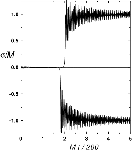
FIG. 1.: A typical evolution of three trajectories in the absence of dissipation with initial conditions separated by a $\pm 10^{-5}$ variation around the $t=0$ values $\phi=4\times\phi_{\rm cr}$, $\dot{\phi}=0$, $\sigma=2\times 10^{-2}M$, $\dot{\sigma}=0$ and $H$ determined by Eq. (6).

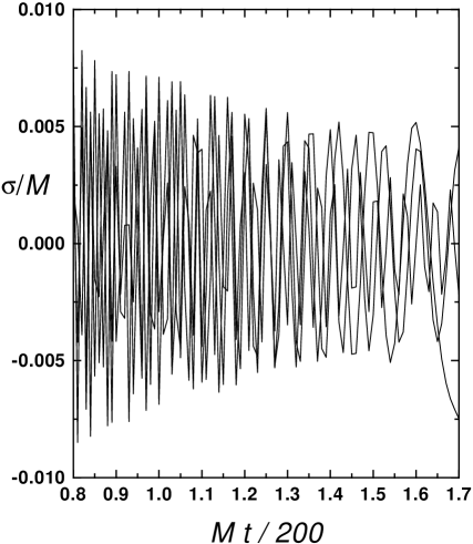
FIG. 2.: A blow-out of the initial time evolution of the trajectories shown in Fig. 1.

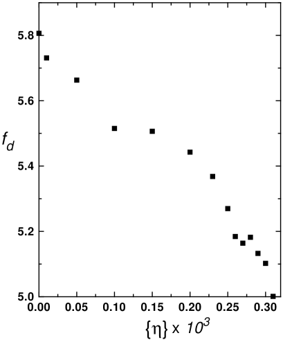
FIG. 3.: The fractal dimension as a function of dissipation, from the box-counting method applied to a box in phase space centered around the initial conditions used in Fig. 1.

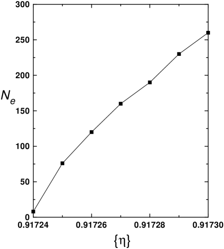
FIG. 4.: The total number of e-folds of inflation as a function of dissipation for the initial conditions at $t=0$: $\phi=3.5M$, $\sigma=M$, $\dot{\phi}=2.5\times 10^{-2}M^{2}$, $\dot{\sigma}=5\times 10^{-4}M^{2}$ and $\rho_{r}(t=0)=0$.

- [1] A. Linde, Phys. Lett. B 259, 38 (1991); M. C. Bento, O. Bertolami and P. M. Sá, Phys. Lett. B 262, 11 (1991); Mod. Phys. Lett. A7, 911 (1992); A. Linde, Phys. Rev. D 49, 748 (1994)
- [2] E. J. Copeland, A. R. Liddle, D. H. Lyth, E. D. Stewart and D. Wands, Phys. Rev. D 49, 6410 (1994); G. Dvali, Q. Shafi and R. Schaefer, Phys. Rev. Lett. 73, 1886 (1994); A. Linde and A. Riotto, Phys. Rev. D 56, 1841 (1997); G. Lazarides, R. K. Schaefer and Q. Shafi, Phys. Rev. D 56, 1324 (1997).
- [3] D. H. Lyth and A. Riotto, Phys. Rep. 314, 1 (1999).
- [4] N. Tetradis, Phys. Rev. D 57, 5997 (1998); G. Lazarides and N. D. Vlachos, Phys. Rev. D 56, 4562 (1997).
- [5] D. S. Goldwirth and T. Piran, Phys. Rep. 214, 223 (1992); T. Vachaspati and M. Trodden, Phys. Rev. D 61, 023502 (2000).
- [6] G. Lazarides and N. Tetradis, Phys. Rev. D 58, 123502 (1998); C. Panagiotakopoulos and N. Tetradis, Phys. Rev. D 59, 083502 (1999).
- [7] L. E. Mendes and A. R. Liddle, Phys. Rev. D 62, 103511 (2000).
- [8] M. Gleiser and R. O. Ramos, Phys. Rev. D 50, 2441 (1994).
- [9] M. Morikawa, Phys. Rev. D 33, 3607 (1986); A. Hosoya and M. A. Sakagami, Phys. Rev. D 29, 2228 (1984).
- [10] D. Boyanovsky, H. J. de Vega, R. Holman, D. -S. Lee and A. Singh, Phys. Rev. D 51, 4419 (1995).
- [11] D. Boyanovsky, R. Holman and S. P. Kumar, Phys. Rev. D 56, 1958 (1997).
- [12] D. Boyanovsky, H.J. de Vega and R. Holman, in Erice Lectures on Inflationary Reheating, presented at International School of Astrophysics, D. Chalonge: 5th Course: Current Topics in Astrofundamental Physics, Erice, Italy (1996), Report No. hep-ph/9701304.
- [13] S.A. Ramsey and B.L. Hu, Phys. Rev. D 56, 678 (1997), Erratum-ibid. D 57, 3798 (1998).
- [14] B. L. Hu, J. P. Paz and Y. Zhang, in The Origin of Structure in the Universe, edited by E. Gunzig and P. Nardone (Kluwer Academic, Norville, 1993); B. L. Hu, J. P. Paz and Y. Zhang, Phys. Rev. D 45, 2843 (1993); ibid D 47, 1576 (1993); E. Calzetta and B. L. Hu, Phys. Rev. D 49, 6636 (1994); ibid D 52, 6770 (1995); B. L. Hu and A. Matacz, Phys. Rev. D 51, 1577 (1995); A. Matacz, Phys. Rev. D 55, 1860 (1997).
- [15] A. Berera, M. Gleiser and R. O. Ramos, Phys. Rev. D 58, 123508 (1998).
- [16] A. O. Caldeira and A. J. Legget, Ann. Phys. 149, 374 (1983).
- [17] H. P. de Oliveira and R. O. Ramos, Phys. Rev. D 57, 741 (1998).
- [18] W. Lee and L.-Z. Fang, Phys. Rev. D 59, 083503 (1999).
- [19] A. Berera and L. Z. Fang, Phys. Rev. Lett. 74, 1912 (1995); A. Berera, Phys. Rev. Lett. 75, 3218 (1995); Phys. Rev. D 54, 2519 (1996); Phys. Rev. D 55, 3346 (1997).
- [20] A. Berera, M. Gleiser and R. O. Ramos, Phys. Rev. Lett. 83, 264 (1999).
- [21] A. Berera and R. O. Ramos, Phys. Rev. D 63, 103509 (2001).
- [22] A. Berera, C. Gordon, Phys. Rev. D 63, 063505 (2001).
- [23] Z. Berezhiani, D. Comelli and N. Tetradis, Phys. Lett. B 431, 286 (1998).
- [24] E. Ott, Chaos in Dynamical Systems (Cambridge University Press, Cambridge 1993).
- [25] N. J. Cornish and J. J. Levin, Phys. Rev. D 53, 3022 (1996); Phys. Rev. D 55, 7489 (1997).
- [26] J. D. Barrow and J. Levin, Phys. Rev. Lett. 80, 656 (1998).
- [27] V. Latora and D. Bazeia, Int. J. Mod. Phys. A 14, 4967 (1999).
- [28] R. O. Ramos and F. A. R. Navarro, Phys. Rev. D 62, 085016 (2000).
- [29] L. G. S. Duarte, L. A. C. P. da Mota, H. P. de Oliveira, R. O. Ramos and J. E. Skea, Comp. Phys. Comm. 119, 256 (1999).
- [30] R. Easther and K. Maeda, Class. Quant. Grav. 16, 1637 (1999).
- [31] B. A. Bassett, Phys. Rev. D 58, 021303 (1998).
- [32] J. Garcia-Bellido and A. Linde, Phys. Rev. D 57, 6075 (1998).
- [33] F. Finelli and R. Brandenberger, Phys. Rev. D 62, 083502 (2000).
- [34] M. Bastero-Gil, S.F. King and J. Sanderson, Phys. Rev. D 60, 103517 (1999).