Mesogranulation and Turbulence in Photospheric Flows

Abstract

Below the scale of supergranules we find that cellular flows are present in the solar photosphere at two distinct size scales, approximately $2$ Mm and $4$ Mm, with distinct characteristic times. Simultaneously present in the flow is a non-cellular component, with turbulent scaling properties and containing $30\%$ of the flow energy. These results are obtained by means of wavelet spectral analysis and modeling of vertical photospheric motions in a 2-hour sequence of 120 SOHO/MDI, high resolution, Doppler images near disk center. The wavelets permit detection of specific local flow patterns corresponding to convection cells.

1 Introduction

The observed velocity field of the solar photosphere falls into two distinct categories. One is acoustic “p-waves” believed to be excited by convective motions [Cox, et al. (1991)]. The p-waves inhabit distinctive ridge-like features in a space-time Fourier spectrum (“$k-\omega$ diagram”) of the motions and can be isolated numerically in a sequence of Doppler images. The other category is flows driven by solar convection. The interaction of convection with the Sun’s rotation produces large-scale flows, such as differential rotation and meridional circulation. These, and giant cells, will not be considered here. The remaining smaller scale flows also contain structure. Most apparent are convection cells with a particular topology: an isolated central upflow surrounded by a multiply connected boundary of downflow [Simon and Weiss (1989)]. These cells favor certain sizes, particularly the granular ($\sim 1-2$ Mm) and supergranular ($\sim 20-40$ Mm) scales. More controversial are the intermediate mesogranular scale ($\sim 4-7$ Mm) and the possible presence of flows that do not have the standard cellular form, that show a continuum of scales between granules and supergranules, and may represent turbulence. In this paper we will argue for the presence in the photosphere of both mesogranular cells and turbulent flows.

Since their discovery [November, et al. (1981)] the sizes and lifetimes of mesogranular cells have proven difficult to determine accurately. For example, correlation tracking of a $45.5$ hour sequence of SOHO/MDI high resolution Doppler images [Shine, et al. (2000)] find mesogranule scales of $5-10$ arcsec ($4-7$ Mm) with lifetimes of a few hours. Similar size scales were estimated by Deubner (1989) on the basis of coherent velocity and intensity fluctuations. Other workers [Ueno and Kitai (1998)] have estimated a characteristic size for mesogranules as large as $18$ arcsec ($13$ Mm) and lifetimes peaking between $30-40$ min. For a listing of other studies see Rieutord, et al. (2000).

Analyses of the photospheric flows in Fourier basis functions or spherical harmonics show broad spectra, with power distributed across all scales between granules and supergranules. For example, Ginet and Simon (1992) show that the Fourier spectrum requires the presence of flow structures at scales $\sim 4-7$ Mm, but they cannot establish that the flow producing this power is cellular or distinct from granules or supergranules. Expansion of both high and low resolution SOHO/MDI Doppler images in spherical harmonics [Hathaway, et al. (2000)] produces very broad spectra with two clear peaks, but with no sign of an intermediate peak signifying mesogranules. It is instead suggested that the spectrum can be decomposed into just two, overlapping, granular and supergranular distributions. The granular distribution would extend over scales from below resolution up to more than $100$ Mm, with a broad peak centered near $3.5$ Mm. The supergranular distribution would extend from $10$ to $300$ Mm in scale with a peak at $\sim 40$ Mm.

Rieutord, et al. (2000) have suggested that different size scales for mesogranules are reported because of different temporal averaging of their respective data sets. Photospheric flows on scales larger than granules may be turbulent and hence composed of flow eddies with sizes obeying a continuous power law distribution. It also is characteristic of steady turbulence that the decorrelation times of eddies increase with their size, also in a power law. Thus, when an observer averages images over some particular period of time, small eddies with a shorter decorrelation time will be suppressed and a characteristic scale will be selected, that might be misinterpreted as mesogranulation.

Here we attempt to resolve this apparent conflict between spectral and correlation tracking analyses by use of wavelet transforms. Wavelets relate the photospheric flow fields to localized basis functions. This has the particular advantage of permitting us to look for particular local configurations in the overall flow field. We will focus on patterns with the particular convection cell topology, that is, isolated areas of upflow (blue shift) bordered by downflow (red shifts). We define this specific pattern to be “cellular” flow. In random flows, this pattern and its reverse should occur with equal probability; in a field of convection cells, this pattern will outweigh its reverse. We determine those size scales for which the correct “cellular” signature exceeds its reverse. In the data set we use, high resolution SOHO/MDI Doppler images at disk center, we will find two, distinct scales of such cellular flows, centered at about $2$ Mm and $4$ Mm ($3$ and $6$ arcsec), and we associate these with granules and mesogranules, respectively. Although the existence of supergranules is well established in horizontal flows, they do not appear readily in our analysis of essentially vertical flows at disk center. However, the presence of spectral power at scales up to $\sim 50$ Mm, with parity between cellular patterns and their reverse, implies that significant non-cellular flows are present. Previous studies by the authors have shown that such structures decorrelate in times which depend on their scales in a power law relationship. In the present case, modeling will further indicate power law spatial correlations for these flows. The scaling properties imply that the non-cellular flows are turbulent.

It thus appears that standard spectral techniques have difficulty resolving mesogranules for three basic reasons: (1) the mesogranules are near in scale to granules and weaker in velocity and (2) they are hidden by overlying turbulence because (3) global basis functions, such as Fourier waves or spherical harmonics, do not allow attention to be paid to the local topologies that label cellular flows. Consequently, determinations of mesogranular scale that do not take into account the specific flow patterns may be contaminated by the non-cellular flows and be artifacts of time averages as suggested by Rieutord, et al. (2000). Nevertheless, when we do look at the specific convective cell pattern, the mesogranules are indeed present, at the small end of the range of previously published sizes.

In Section 2 we describe the data set employed in this paper. In section 3 we give a brief summary of continuous wavelet analysis, and in Section 4 this is applied to observed photospheric flow fields. In Section 5 we construct a model flow field and compare the generated spectra to the observed case. Conclusions are presented in Section 6.

2 Data

The data are SOHO/MDI, high resolution, Doppler images [Scherrer, et al. (1995)]. They consist of a $120$ min sequence of consecutive, $1$ min cadence, $1000$ pixels east-west by $600$ pixels north-south, Doppler images made on 1997 February 5. The pixel scale is $0.625$ arcsec or $0.46$ Mm on the Sun. The images were defocused to avoid aliasing. To remove p-waves we used a previously determined optimal acoustic filter [Lawrence, et al. (1999)]: keeping in the $k-\omega$ diagram only spatial frequencies $k>5\omega-15$, where $k$ is in pixels^-1, and the temporal frequency $\omega$ is in minutes^-1. So as to concentrate on vertical photospheric motions we restricted our attention to a region within $75$ pixels = $34$ Mm of the disk center. Figure 1 shows an individual Doppler image at the middle of the sequence, together with an average of the 120 images spanning two hours in time. Note that the features in the averaged image are larger in scale than those in the individual image.

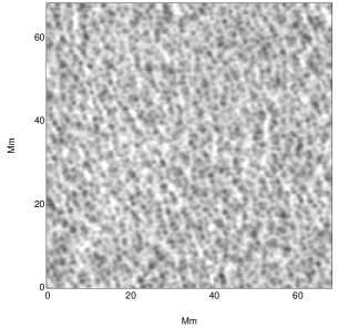
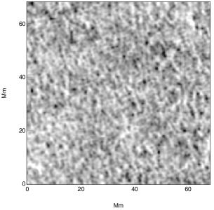
a.   Individual Image b.   120 Min. Average

Figure 1: a. Single SOHO/MDI, acoustically filtered, Doppler image of vertical flows near disk center. b. An average of the 120 images spaced at 1 min intervals and spanning two hours in time. In these images red shifted downflows appear light and blue shifted upflows appear dark.

For images like those in Figure 1, we express the vertical velocity of the photosphere in km s^-1 as a function of position on the solar surface: $v(\mathbf{r})$. The convention for the SOHO/MDI Doppler images is that for red shifted downflows $v>0$; for blue shifted upflows $v<0$.

3 Wavelet Analysis

The methods used here are described in more detail in Lawrence, et al (1999). In two spatial dimensions a continuous wavelet transform $W(s,\mathbf{x})$ of a function $v(\mathbf{r})$ is its convolution with scaled and translated versions of a basis function $\Psi(\mathbf{r})$:

$$W(s,\mathbf{x})=\frac{1}{s}\int v(\mathbf{r})\Psi(\frac{\mathbf{r-x}}{s})d^{2}\mathbf{r.}$$ (1)

Note that the transform adds a scale variable $s$ to the position variable $\mathbf{x}$. The basis function must be localized in both Fourier space ($\mathbf{k}$) and configuration space ($\mathbf{r}$), so that equation (1) gives a strong response to structure in $v(\mathbf{r})$ of scale $s$ at position $\mathbf{x}$ and a weak response otherwise.

A variety of basis functions are acceptable. For determining spectra will use a sixth order function with radial symmetry:

$$\Psi_{6}(r)=-\nabla^{2}\nabla^{2}\nabla^{2}\exp(-r^{2}/2),$$ (2)

or in Fourier space

$$\widetilde{\Psi}_{6}(k)\propto k^{6}\exp(-k^{2}/2).$$ (3)

This wavelet strongly suppresses both small and large scale (respectively, large and small $k$) contributions and thus gives good resolution in scale [Perrier, et al. (1995)].

The global wavelet spectrum of an image may be expressed [Farge (1992)] as

$$\mathcal{E}_{W}(s)=\frac{1}{s^{2}}\int\left|W(s,\mathbf{x})\right|^{2}d^{2}\mathbf{x,}$$ (4)

where $\left|W(s,\mathbf{x})\right|^{2}/s^{2}$ is the  energy density as a function of scale and position. The global energy spectrum is related to the Fourier transform $\widetilde{v}(\mathbf{k})$ of $v(\mathbf{r})$  and the Fourier energy density $\mathcal{E}_{F}(\mathbf{k})=\left|\widetilde{v}(\mathbf{k})\right|^{2}$ by

$$\mathcal{E}_{W}(s)=\int\mathcal{E}_{F}(\mathbf{k})\left|\widetilde{\Psi}(s\mathbf{k})\right|^{2}d^{2}\mathbf{k,}$$ (5)

where $\widetilde{\Psi}$ is the Fourier transform of $\Psi$. Thus $\mathcal{E}_{W}(s)$ is the Fourier energy density, smoothed by the Fourier spectrum of the wavelet basis function at each scale. The information it carries is similar to that carried by the Fourier density, but with lower resolution in scale or spatial frequency.

4 Data Analysis

4.1 Fourier Spectra

The total power in an image may be written

$$E=\int d^{2}k\left|\widetilde{v}(\mathbf{k})\right|^{2}=\int_{0}^{\infty}dkk\int_{0}^{2\pi}d\phi\mathcal{E}_{F}(k)$$ (6)

Here $k=\left|\mathbf{k}\right|$ and $\phi$ are polar coordinates in Fourier space. For the 2-dimensional images the Fourier power spectrum $E_{F}(k)$, or power per unit wave number, is

$$E_{F}(k)=dE/dk=k\int_{0}^{2\pi}d\phi\mathcal{E}_{F}(k),$$ (7)

where we assume statistical isotropy. For a white noise image $E_{F}(k)\propto k$, and for Kolmogorov turbulence $E_{F}(k)\propto k^{-2/3}$. Here we make use only of squares of side $256$ pixels = $116$ Mm centered on disk center. Figure 2 depicts the average of the Fourier spectra of the image centers. The $1\sigma$ error bars are derived from the scatter in the spectra of invividual images spaced at 10 minute intervals. This allows some randomization and statistical independence in the small scales.

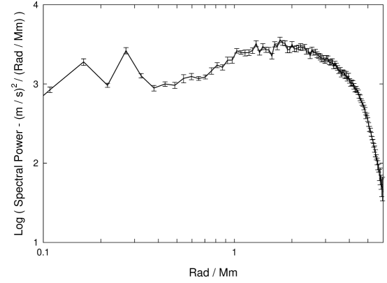
Figure 2: $E_{F}(k)$ Fourier power spectrum. The error bars are derived from the average over individual spectra.

We will use the Fourier spectrum to calibrate the spectral power of the wavelet spectra.

4.2 Wavelet Spectra

We compute the convolutions of the images with the $\Psi_{6}$ basis function according to equation (1) and the wavelet energy density according to equation (4). The spectra will be plotted as functions of spatial frequency $k=2\pi/s$, and transformed to the format of a Fourier spectrum, that is, as power per unit wavenumber $k$. The resulting wavelet power spectrum, as in equation (7), is

$$E_{W}(k)=k\int_{0}^{2\pi}\mathcal{E}_{W}(k)d\phi,$$ (8)

although calculated with wavelets, is directly comparable to the Fourier spectrum $E_{F}(k)$.

Two kinds of wavelet spectra are computed. Since the wavelet basis function is a positive central peak with radial ripples around it, the wavelet transform $W(s,\mathbf{x})$ of a convection cell, with a central $v<0$ upflow and peripheral $v>0$ downflow, will be negative at the cell’s scale $s$ and position $\mathbf{x}$. In the case of a random flow field, $W(s,\mathbf{x})$ at a given scale and location will be positive or negative with equal probability. If convection cells also are present in the flow there will be an excess of negative values around the corresponding locations and scales.This local feature of the wavelet transforms is what we use to look for mesogranulation.

We compute, within $34$ Mm of the disk center, the wavelet spectrum $E_{W}^{+}(k)$ using only the positive values of $W(s,\mathbf{x})$. Likewise, we compute the spectrum $E_{W}^{-}(k)$ including only the negative values. The $E_{W}^{+}(k)$ spectrum will include essentially no contributions from convective “cells” (which correspond to $W<0$), but only non-cellular contributions. The $E_{W}^{-}(k)$ spectrum will include both cellular and non-cellular contributions. Because of the locality property of the wavelets, the sum $E_{W}(k)=E_{W}^{-}(k)+E_{W}^{+}(k)$ is just the full wavelet spectrum and is a smoothed version of the Fourier spectrum as described above. The difference of the two spectra $E_{C}(k)=E_{W}^{-}(k)-E_{W}^{+}(k)$ will characterize the cell scales. Recall that $E_{W}^{-}(k)$ contains all the cellular contributions. The non-cellular “background” is, at least statistically, subtracted off with $E_{W}^{+}(k)$. Those scales $s=2\pi/k$ for which $E_{C}(k)$ is significantly positive will be those scales at which convection cells are present in the photospheric images. The average of the $E_{W}(k)$ spectra of the 120 images and the corresponding average cellular $E_{C}(k)$ spectrum are shown in Figure 3.

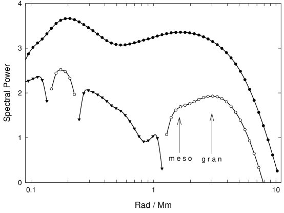
Figure 3: Filled circles: average of the wavelet power spectra $E_{W}(k)$ of the 120 photospheric images. Open circles: positive part of the average of the cellular spectra $E_{C}(k)$ of the images. Filled triangles: average of the negative part of the cellular spectra. This indicates the relative significance of positive excursions of $E_{W}$. The power is calibrated to the corresponding Fourier spectrum in Figure 2.

Figure 3 shows the full $E_{W}(k)$ spectrum as filled circles. Shown as open circles are the parts of the cellular spectrum for which $E_{C}(k)>0$. Shown as filled triangles are the absolute values of those parts of the cellular spectrum for which $E_{C}(k)<0$. These last parts characterize the non-cellular, background flows. Their negative slope indicates strong large scale correlations in the stochastic background. The $E_{C}>0$ feature near $k=0.2$ Rad Mm^-1, though suggestively near $30$ Mm in size, is not sufficiently strong to represent supergranules, but represents non-cellular, large scale correlation features. This will be discussed further below, when we model the flows. The cellular spectrum in Figure 3 does, however, indicate the presence of two characteristic spatial scales: at $\sim 2$ Mm corresponding to granules and at $\sim 4$ Mm representing mesogranules.

4.3 Decorrelation Times

Figure 4 shows as a solid line a magnified view of the granular and mesogranular cellular $E_{C}(k)$ spectrum. Recall that this is taken from an average over the individual spectra of all 120 of the Doppler images. It thus characterizes the stationary flow as seen at a typical point in time. Shown in Figure 4 as the long dashed line is an analogous spectrum made by first averaging the 120 images and then calculating the cellular spectrum. Because this average spans $2$ hr in time, features with coherence times $\lesssim 2$ hr are blurred, and the spectral power is accordingly reduced. The granular feature at $k\approx 3.14$ Rad Mm^-1 ($s\approx 2$ Mm) has decayed by an order of magnitude, much more than the mesogranular feature at $k\approx 1.57$ Rad Mm^-1 ($s\approx 4$ Mm). In fact, the mesogranular peak now dominates the granular one.

Also shown in Figure 4 are plots of the average of six spectra made from $20$ min averages of images, the average of three spectra made from $40$ min averages of images, and the average of three spectra made from (overlapping) $60$ min image averages. These allow us to trace the evolutionary timescales of the cellular features. The granular feature is already decayed in the $20$ min averages and has dropped by a factor $\sim 3$ in the $40$ min averages. The mesogranular feature has not decayed essentially at all in the $40$ min averages and is larger than the granular feature. By the $60$ min image average the mesogranules are evolving too, and their peak is decreasing. Thus we see that, in addition to distinct spatial scales, there are distinct, non-overlapping, coherence times for the granules (less than $20$ min) and the mesogranules (more than $40$ min).

The essential difference between this result and the suggestion of Rieutord, et al. (2000) is that averaging of images over various time periods does not select from a continuum of cellular scales, but rather from two scales. For short averaging times the granular scale $2$ Mm is selected. For longer times the mesogranular scale $4$ Mm is selected.

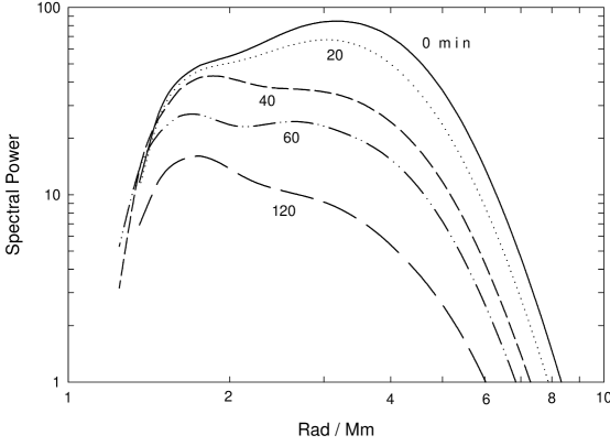
Figure 4: Solid line: average of the cellular spectra of each of the 120 Doppler images. Dotted line: Average of the cellular spectra of six image averages spanning $20$ min each. Short-dashed line: Average of spectra of three image averages spanning $40$ min each. Dot-dash line: Average of spectra of three overlapping image averages spanning $60$ min each. Long-dashed line: spectrum of an average over all 120 images spanning $120$ min.

5 Modelled Data

To extend the interpretation of the observational results, we construct a model photospheric velocity field. This is intended to apply to the velocities at a typical moment in time and includes no evolution. We represent a model “cell” by the negative of a “Mexican hat” wavelet basis function in the form

$$\Psi_{M}(r)=V(1-r^{2}/2a^{2})\exp(-r^{2}/2a^{2})$$ (9)

This models a central blue shifted feature with characteristic radius $a$ surrounded by a red shifted ring with maximum downflow at radius $2a$. We take the diameter $4a$ to be the “size” of a cell with scale parameter $a$. On an array of $1024$ pixels $\times$ $1024$ pixels we randomly locate with uniform probability $32,768$ “granular” wavelets with scale $a=3$ pixels and central vertical velocity $V=110$ ms^-1 and $3,640$ “mesogranular” wavelets with $a=6$ pixels and $V=45$ ms^-1. As we will see, this models well the granular and mesogranular parts of the cellular spectrum if we choose $a=0.5$ Mm. The numbers of model granules and mesogranules included are based on the numbers that would be contained in square arrays with separations $3a-4a$.

To model the observed spectral power at scales $\gtrsim 4$ Mm ($k\lesssim 1.57$ Rad Mm^-1) requires a non-cellular flow component with a continuous range of scales. To model the correct slope for the spectra it is necessary to use “colored” noise with increased spatial correlations at large scales. We first generate a Gaussian white noise image. Then we transform to Fourier space and multiply the transform by $k^{-\gamma}$ with cutoffs in scale $s=2\pi/k<$ $4$ pixels and $s>$ $256$ pixels. The negative exponent emphasizes larger scales. The spectrum of this colored noise has a power law form $E(k)\propto k^{1-2\gamma}$. The best fit to solar data is given by a value $\gamma=0.6$, giving the spectrum $E(k)\propto k^{-0.2}$. To get the image noise we transform back to configuration space. The standard deviation of the colored noise used in the model was $42$ ms^-1.

The cellular and stochastic velocities quoted here were obtained by calibrating the overall image variance in Figure 5a to that of Figure 1a. The variance of the cellular component of the model image is $4800$ m²s^-2, and that of the stochastic component is $1800$ m²s^-2. This implies that the stochastic component contains $\sim 30\%$ of the variance and hence kinetic energy of the model flow.

An artificial cell-plus-noise velocity field created in this way is illustrated in Figure 5a. An image of the colored noise alone is shown in Figure 5b.

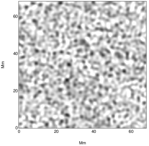
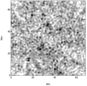
a.   Modeled Image b.   Colored Noise

Figure 5: a. Image of artificial flow field constructed from two discrete cell sizes and spatial colored noise. b. The colored noise used in (a). Note the long range spatial correlations.

The wavelet spectra generated by the modelled velocity field in Figure 5a are shown in Figure 6 in comparison to the solar data. The filled circles indicate $E_{W}(k)$ for the solar data, and the open circles the positive part of $E_{C}(k)$ for the solar data. The solid line is $E_{W}(k)$ for the modelled data, and the dashed lines give $E_{C}(k)$ for the modelled data. The slopes for the full $E_{W}(k)$ spectra are in general agreement at all scales.

The observed and modelled cellular spectra of the granules and mesogranules agree very well for wave numbers $1$Rad Mm${}^{-1}<k<10$ Rad Mm^-1. The resolution of $E_{C}(k)$ is such that the granular and mesogranular peaks overlap. We know, however, by construction, that the granular and mesogranular scales in the modelled image are discrete. It follows that these scales in the solar data may well also be discrete. Attempts to model the observed cellular spectrum with a continuum of cell sizes between $2$ Mm and $4$ Mm were unsuccessful.

The particular realization of the modelled data shown here shows a structure near $k\approx 0.2$ Rad Mm^-1 or scale $\sim 30$ Mm. Again by construction, the modelled image contains no supergranules. This structure must therefore represent large scale correlations in the stochastic component of the modelled flow. Accordingly, we interpret the comparable feature in the observed spectrum as a large scale correlation feature of the non cellular-flow, rather than as supergranular. Recall that the spectrum of the background “noise” has slope $-0.2$.

Figure 7 shows the same full wavelet spectra of the observed and modelled solar flows that are shown in Figure 6. Also shown are other modelled spectra constructed with no added stochastic component (long dashed line) and with a white noise ($\gamma=0$) stochastic component (short dashed line). Neither of the last two is able to approximate the observed spectrum at large scales ($k\lesssim 1$ Rad Mm^-1).

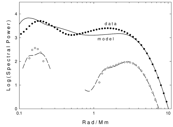
Figure 6: Filled circles: Average of the full $E_{W}(k)$ wavelet spectra of all 120 images. Open circles: Average of the positive parts of the cellular $E_{C}(k)$ spectra over all 120 images. Solid Line: $E_{W}(k)$ spectrum of the modelled image of Figure 5a. Dashed line: Positive parts of the $E_{C}(k)$ spectrum of the modelled image. Frequency units have been adjusted to Rad Mm^-1 by calibration with the observed spectra.

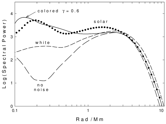
Figure 7: Filled circles: Average of the full $E_{W}(k)$ wavelet spectra of the 120 solar images. Solid line: Full $E_{W}(k)$ spectrum of the modelled image of Figure 5a made with a colored noise stochastic component. Short-dashed line: $E_{C}(k)$ spectrum for the same modelled image, but with a white noise stochastic component. Long-dashed line: $E_{W}(k)$ spectrum of the same modelled image, but with no stochastic component. Frequency units have been adjusted to Rad Mm^-1 by calibration with the observed spectra.

6 Discussion and Conclusions

The cellular spectra of the SOHO/MDI Doppler images cannot be explained without two discrete cellular components: granules with size scale $\sim 2$ Mm and coherence time less than $20$ min and mesogranules with size scale $\sim 4$ Mm and coherence time greater than $40$ min. There is no evidence that the granules and mesogranules overlap significantly in scale. We note that the convective cells visible in Figure 1b are noticeably larger than in Figure 1a and, based on our analysis, depict mesogranules.

The photospheric velocity spectrum can be reproduced in all its essential aspects by adding to the modelled cellular flows a stochastic component with power law spatial correlations, resembling those of turbulence, and containing $\sim 30\%$ of the flow energy. In earlier work [] we found that the stochastic component of vertical flows in high resolution SOHO/MDI Doppler images displayed decorrelation times that scaled as a power law with spatial frequency. These two kinds of scaling indicate fluid turbulence. We have found a best fit spatial spectral index $\gamma=0.6$ which is similar to the $\gamma\approx 0.83$ which would signify Kolmogorov turbulence. Previous work by the authors [] has indicated $\gamma\approx 0.83$ for horizontal flows from SOHO full disk data for scales greater than $16$ Mm ($k<0.4$ Rad Mm^-1). The horizontal flows also show temporal decorrelation scaling over scales $3.6$ Mm $\leq s\leq$ $120$ Mm. Similar results were found still earlier [Ruzmaikin, et al. (1996)] for a sequence of San Fernando Observatory Doppler images.

With a photospheric Reynolds number $\sim 10^{8}$ the presence of turbulence should be no surprise. The co-existence of stochastic flows and coherent structures determined by boundary conditions is a hallmark of turbulence in nature [Holmes, et al. (1996)]. We thus suggest that, after careful filtering for p-waves, the photospheric flows indeed fall into both of these categories. The cellular flows appear to be present at discrete scales which must be determined in some way by convective boundary conditions. The textbook explanation in terms of the recombination depths of hydrogen at 1 Mm and of helium at 5 Mm and 15 Mm (for supergranules) [Simon and Weiss (1968)] remains viable.