Non-gaussian CMB temperature fluctuations from peculiar velocities of clusters

Abstract

We use numerical simulations of a (480 Mpc$/h$)³ volume to show that the distribution of peak heights in maps of the temperature fluctuations from the kinematic and thermal Sunyaev-Zeldovich effects will be highly non-Gaussian, and very different from the peak height distribution of a Gaussian random field. We then show that it is a good approximation to assume that each peak in either SZ effect is associated with one and only one dark matter halo. This allows us to use our knowledge of the properties of haloes to estimate the peak height distributions. At fixed optical depth, the distribution of peak heights due to the kinematic effect is Gaussian, with a width which is approximately proportional to optical depth; the non-Gaussianity comes from summing over a range of optical depths. The optical depth is an increasing function of halo mass, and the distribution of halo speeds is Gaussian, with a dispersion which is approximately independent of halo mass. This means that observations of the kinematic effect can be used to put constraints on how the abundance of massive clusters evolves, and on the evolution of cluster velocities. The non-Gaussianity of the thermal effect, on the other hand, comes primarily from the fact that, on average, the effect is larger in more massive haloes, and the distribution of halo masses is highly non-Gaussian. We also show that because haloes of the same mass may have a range of density and velocity dispersion profiles, the relation between halo mass and the amplitude of the thermal effect is not deterministic, but has some scatter.

1 Introduction

The inverse Compton scattering of free electrons in the intracluster plasma with the photons of the cosmic background radiation produce secondary fluctuations in background radiation temperature maps. The electron motion is due both to thermal motions within the plasma, and to coherent bulk motions of the plasma (e.g. Sunyaev & Zeldovich 1980). Simulations suggest that the distribution of these temperature fluctuations will be quite non-Gaussian (Seljak, Burwell & Pen 2001), and that the best hope of detecting this effect is in the tails of the distribution (e.g. da Silva et al. 2000). In this paper, rather than studying the distribution of temperature fluctuations in random pixels, we study the distribution of fluctuations in pixels which are peaks. We show that the distribution of these peak heights should be highly non-Gaussian, and that the exact shape can be computed if the spectrum of initial density fluctuations is known. Comparison with estimates of the peak height distribution from large $n$-body simulations shows that our model is quite accurate. This means that observations of the peaks alone should allow one to place constraints on what the initial conditions must have been. In this paper, we restrict attention to the simplest case in which signals come from a single redshift, chosen to be close to the present epoch, when nonlinear structures have already grown. Work in progress studies contributions from higher redshifts; even when a range of redshifts contribute, our conclusion that the final distribution of fluctuations should be non-Gaussian, and related to the initial density fluctuation distribution, should remain unchanged.

This paper is organized as follows. Section 2 describes our simulations briefly. Section 3 studies the kinematic effect, and Section 4 studies the thermal effect. The thermal effect is closely related to the optical depth, and so this section also includes a study of the optical depth distribution. A final section summarizes our findings.

2 The simulations

The simulation we will use was recently carried out by the Virgo Consortium. It uses $512^{3}$ particles in a cosmological box of $480h^{-1}$Mpc on a side. The cosmological model is flat with matter density $\Omega_{0}=0.3$, cosmological constant $\Omega_{\Lambda}=0.7$ and expansion rate at the present time $H_{0}=70$km^-1Mpc^-1. It has a CDM initial power spectrum computed by CMBFAST (Seljak & Zaldarriaga 1996), normalized to the present abundance of galaxy clusters so that $\sigma_{8}$=0.9. We emphasize that, if the kinematic effect arises from the peculiar velocities of clusters, then a large simulation box such as ours is essential for studying this effect: smaller boxes miss a significant fraction of the power which generates velocities, so they are liable to underestimate the magnitude of the effect (see Sheth & Diaferio 2001 for more discussion on the finite box size effect). In addition, our large simulation contains a large number of massive haloes which smaller simulation boxes are likely to misestimate. The proper population of massive halos is essential for studying the distribution of the thermal effect (e.g. Refregier & Teyssier 2000).

From the simulation outputs we create maps of the thermal SZ effect, the kinematic SZ effect, and the Thomson optical depth. We compute the local gas density and velocity from those of dark matter, and the gas temperature is computed from the local dark matter velocity dispersion, following the procedure outlined in Diaferio, Sunyaev, & Nusser (2000). We project the simulation box on a fine 2400² grid in a random direction; thus, each pixel in the grid is $L=200h^{-1}$kpc on a side. This pixel scale $L$ is about an order of magnitude larger than the 30$h^{-1}$kpc spatial resolution of the simulation.

Figure 1: Scatter plot showing the height of a $k_{\rm SZ}$ peak as a function of optical depth $\tau$.

3 The kinematic effect

The optical depth is defined by

$$\tau=\sigma_{\rm T}\int n_{\rm electron}(l)\ {\rm d}l\approx{\sigma_{\rm T}\over m_{\rm proton}}{\Omega_{\rm b}\over\Omega_{0}}\rho_{\rm crit}\int{\rm d}l\ {\rho_{\rm dm}(l)\over\rho_{\rm crit}},$$ (1)

where $\sigma_{\rm T}$ is the Thomson scattering cross-section, $n_{\rm electron}(l)$ is the density of electrons along the line of sight at $l$, $\rho_{\rm dm}(l)$ is the mass density along the line of sight at $l$, $\rho_{\rm crit}\Omega_{0}$ is the average mass density of the background, and $\Omega_{\rm b}$ denotes the abundance of baryons. In what follows we have set $\Omega_{\rm b}=0.0125/h^{2}$. The second equality shows the approximations used by Diaferio, Sunyaev & Nusser (2000) to relate the properties of the dark matter particles in their simulations to those of the gas: the gas traces the dark matter.

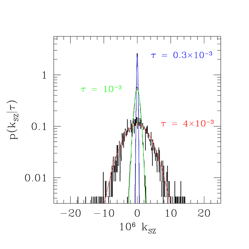
Figure 2: Distribution of $k_{\rm SZ}$ peak heights at fixed optical depth. Curves show Gaussians with the same rms.

The kinematic effect temperature fluctuation $k_{\rm SZ}$ is defined by

$$k_{\rm SZ}={\Delta T\over T}={\Omega_{\rm b}\over\Omega_{0}}{\sigma_{\rm T}\over m_{\rm proton}}\rho_{\rm crit}\int{\rm d}l\ {\rho_{\rm dm}(l)\over\rho_{\rm crit}}\,{v(l)\over c_{\rm light}},$$ (2)

where $v(l)/c_{\rm light}$ is the bulk velocity along the line of sight at $l$, divided by the speed of light. Notice that if one thinks of the optical depth as a measure of the density, then the kinematic effect is a measure of the momentum. Below, we first describe what is seen in simulations of the kinematic effect, and then we present a model which provides a reasonably good fit to the simulations.

Diaferio et al. (2000) presented a study of peaks in their simulated maps of the thermal and kinematic SZ effects. The panels on the left of their Figure 3 show that the mean peak height for the thermal SZ effect scales with the square of $\tau$, the optical depth: $t_{\rm SZ}\equiv\Delta T(K)/T(K)=-2\tau^{2}$. We will consider this in the next section. This section is devoted to a study of the relation presented in the panels on the right of their Figure 3.

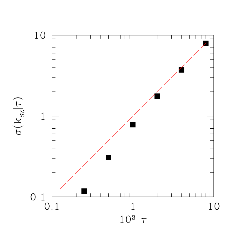
Figure 3: The rms value of $k_{\rm SZ}$ at fixed $\tau$ as a function of $\tau$. Dashed line shows the scaling expected if $\sigma(k_{\rm SZ}|\tau)$ increases linearly with optical depth.

Fig. 1 shows our version of their Figure 3: it shows the heights of the peaks in the kinematic effect, $k_{\rm SZ}$, as a function of optical depth. It was constructed following the procedures Diaferio et al. outlined; the only difference is that here we use a $\sim$40 times larger simulation described in the previous section. Notice that the mean $k_{\rm SZ}$ peak height is zero for all $\tau$, but the scatter around zero increases as $\tau$ increases. Fig. 2 shows that, at fixed $\tau$, the distribution around the mean is well fit by a Gaussian. To a good approximation, the width of the Gaussian increases linearly with $\tau$. This is shown in Fig. 3. The distribution of the peak heights is got by integrating over all $\tau$:

$$p(k_{\rm SZ})=\int{\rm d}\tau\,p(\tau)\,G(k_{\rm SZ}|\tau),$$ (3)

where $G$ denotes the Gaussian distribution of $k_{\rm SZ}$ at fixed $\tau$. Because the width of the Gaussian depends strongly on $\tau$, the resulting $p(k_{\rm SZ})$ is a summation of Gaussians of different dispersions. This is the fundamental reason why the distribution $p(k_{\rm SZ})$ is likely to be highly non-Gaussian. The histogram in Fig. 4 shows this distribution—note how centrally cusped it is.

In what follows, we will describe why the distribution of $k_{\rm SZ}$ at fixed $\tau$ is Gaussian, and why $\sigma(k_{\rm SZ}|\tau)\propto\tau$. We will then provide a model for $p(\tau)$. When inserted into the expression above, these ingredients allow us to model the distribution of $k_{\rm SZ}$—this produces the solid curve shown in Fig. 4.

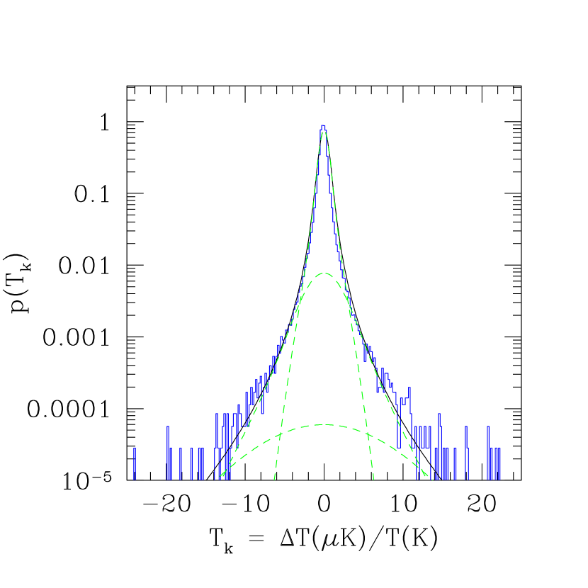
Figure 4: Distribution of $k_{\rm SZ}$ fluctuations from sources at $z=0$. Histogram shows the measurements in the $n$-body simulation, solid curve shows what our model predicts (eq. 11 below). Dashed curves show the predicted contribution to the solid curve from haloes with mass in the range $10^{12}-10^{13}$ (narrowest distribution), $10^{13}-10^{14}$, and $10^{14}-10^{15}M_{\odot}/h$ (broadest distribution with lowest peak).

3.1 The model

If we think of the integral along the line of sight $l$ as a sum over discrete pixels, then we can ask how the density and the velocity in pixels change as we step through $l$. As we do this, it is likely that some pixels along the line of sight will contain, or lie within, dark matter haloes. Because the virial motions within haloes are random, the component of $v(l)$ which is due to the virial motions will fluctuate around zero. The result of integrating over all $l$ is that these internal virial motions will cancel out, so only the bulk peculiar velocities of the haloes contribute to the line of sight integration. In addition, there may be contributions to the integral from pixels which do not contain haloes. However, the density within a halo is on the order of two hundred times $\rho_{\rm crit}$. So, provided that the motions of haloes are not significantly smaller than the motions in less dense regions, and provided that velocities are not correlated over scales which are on the order of two hundred times larger than the size of a typical halo, pixels associated with haloes contribute much more to the line of sight integral than do the much less dense pixels which have nothing to do with haloes. In this respect, our analysis is similar to that in Cole & Kaiser (1988) and Peebles & Juszkiewicz (1998).

Haloes are rare, so, for sufficiently small pixels, it is unlikely that a given line of sight will contain more than one halo. Moreover, the haloes have central density cusps (e.g. Navarro, Frenk & White 1997). Therefore, peaks in the $k_{\rm SZ}$ distribution occur in those pixels which contain the density cusps. We assume that there is one density cusp per halo, so the number density of peaks in the $k_{\rm SZ}$ distribution should approximately equal the number density of haloes. Moreover, we can replace the integral over the line of sight by the value the integrand had at the position of the peak:

$$k_{\rm SZ}=\left({v\over c_{\rm light}}\right)\ {\Omega_{b}\over\Omega_{0}}{\sigma_{\rm T}\over m_{\rm proton}}\rho_{\rm halo}\,R_{\rm halo}=(v/c_{\rm light})\,\tau,$$ (4)

where $v$ is the bulk velocity of the halo, $c_{\rm light}$ is the speed of light, $\rho_{\rm halo}$ and $R_{\rm halo}$ are intended to denote the average density contributed by the halo over the range of pixels along the line of sight, $R_{\rm halo}$, it occupied. The final expression defines $\tau$, the optical depth of the pixel containing the central density cusp of the halo. So, to model the distribution of $k_{\rm SZ}$, we must be able to model how the optical depth $\tau$ and the velocity $v$ depend on halo mass $m$. In addition, we must be able to estimate the number density $n(m)$ of haloes.

The optical depth in a square pixel of side $L$ which contains the central density cusp of a halo of mass $m$ and central concentration parameter $c$, can be estimated by setting

$$\tau(m)=2\,\int_{0}^{W}{{\rm d}w\over W}\,{w\over W}\,\tau(w|c,m),$$ (5)

where $W=[L/r_{\rm s}(m)]/\sqrt{\pi}$, and

$$\tau(w|c,m) = {\sigma_{\rm T}\over m_{\rm proton}}{\Omega_{\rm b}\over\Omega_{0}}\,r_{\rm s}\int{\rm d}l\ \rho(x|c,m)$$ (6)

$$= {\sigma_{\rm T}\over m_{\rm proton}}\,{\Omega_{\rm b}\over\Omega_{0}}\,r_{s}(m)\rho_{s}(m)\,{2[1-h(w)]\over w^{2}-1}$$

(e.g. Cramphorn 2001). This expression for $\tau(w|m)$ is got by expressing all distances in units of $r_{s}(m)$ and then projecting a Navarro, Frenk & White (1997) profile along the line-of-sight:

$$\rho(x|c,m) = {\rho_{\rm s}\over x(1+x)^{2}},\qquad{\rm where}\ x^{2}=l^{2}+w^{2},$$

$$\rho_{\rm s}(m) = \rho_{\rm crit}\delta_{c}(m)$$

$$= \rho_{\rm crit}{\Delta_{\rm nl}\over 3}{c^{3}(m)\over\ln[1+c(m)]-c(m)/[1+c(m)]},$$

$$r_{\rm s}(m) = {r_{\rm vir}\over c(m)}={1\over c(m)}\left({3m\over 4\pi\rho_{\rm crit}\Delta_{\rm nl}}\right)^{1/3},$$

$$c(m) = 12\left({m\over m_{*}}\right)^{-0.13},$$

$$h(w) = {{\rm arccosh}(1/w)\over\sqrt{1-w^{2}}}\quad\mbox{if $w\leq 1$}$$ (7)

$$= {\arccos(1/w)\over\sqrt{w^{2}-1}}\ \quad\mbox{if $w>1$},$$

and $\Delta_{\rm nl}\approx 100$ for the $\Lambda$CDM model we are considering here. The quantity $c(m)$ is often called the concentration parameter of the halo. Massive haloes are less centrally concentrated (Navarro, Frenk & White 1997); we use the parametrization of this mass dependence given by Bullock et al. (2001). The final averaging over the circular beam of radius $W$ can also be done analytically:

$$\tau(m)={\sigma_{\rm T}\over m_{\rm proton}}\,{\Omega_{\rm b}\over\Omega_{0}}\,r_{\rm s}(m)\rho_{\rm s}(m)\,{2\over W^{2}}\,\Bigl{[}\ln\left({W^{2}/4}\right)+2h(W)\Bigr{]}.$$ (8)

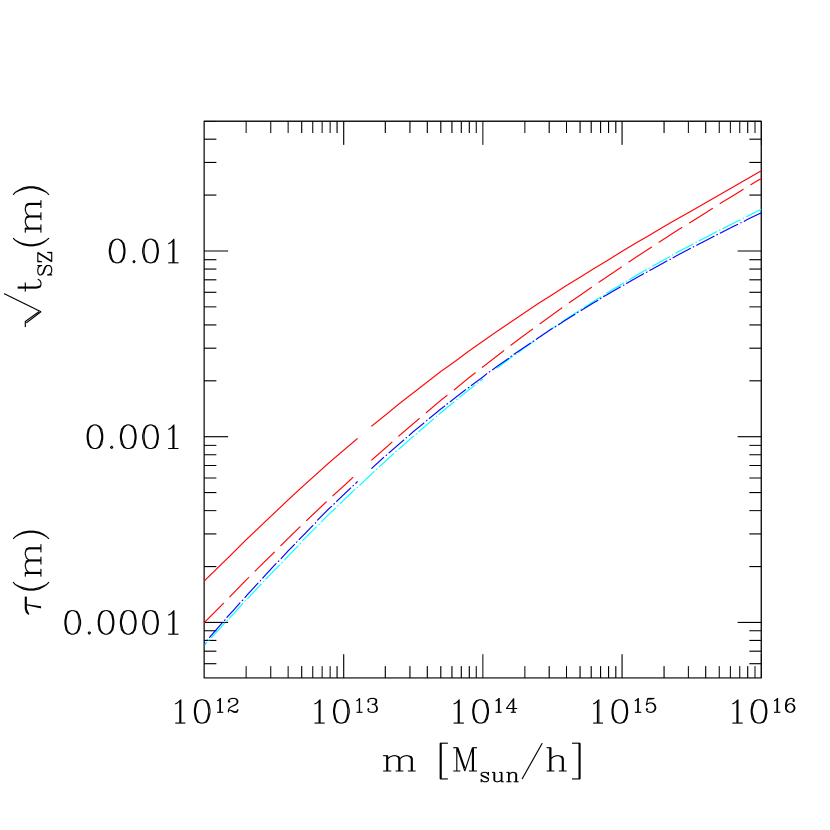
Figure 5: Optical depth $\tau$ and thermal SZ effect $t_{\rm SZ}$ peak heights as functions of halo mass $m$. Lower dot-dashed curves show $\tau(m)$ for profiles of the form given by Hernquist (1990) and by Navarro et al. (1997). Upper solid and dashed curves show $\sqrt{|t_{\rm SZ}|}$ for Hernquist profiles when the circular velocity and the isotropic dispersion, respectively, are used to estimate the temperature.

One of the dot-dashed curves in Fig. 5 shows the optical depth given by equation (8). Notice that, for low mass haloes, $L\gg r_{\rm s}$, and the term in square brackets in equation (8) tends to a constant. In this limit $\tau\propto r_{s}^{3}\rho_{s}$ (recall that $W^{2}\propto r_{\rm s}^{-2}$), which means that the optical depth is approximately proportional to $m$. This is sensible, since, in this limit, the entire halo fits in the cell. The more massive haloes have larger scale radii and so they also have larger optical depths; at large $m$, $\tau(m)$ is approximately proportional to $m^{2/3}$ (see Fig. 5). For our purposes in this section, the important point is that the optical depth is a monotonically increasing function of halo mass.

To show that this conclusion is not terribly sensitive to the details of the density run in the outer regions of haloes, the other dot-dashed curve shows the optical depth associated with the profile shape presented in Hernquist (1990). The Appendix shows that, for this profile shape also, the relevant integrals can all be computed analytically. (We will describe the other two curves in the next section.) The Hernquist profile scales as $1/x/(1+x)^{3}$; although it falls more steeply at large radii, it has the same small scale slope as the Navarro et al. profile. The fact that the optical depths for these two parametrizations of halo profile shapes are so similar shows that most of the contribution to the optical depth comes from the inner parts of the haloes, where the profiles themselves are similar.

What about halo speeds? Sheth & Diaferio (2001) showed that, if the initial density fluctuation field was Gaussian, then to a good approximation, the speeds of dark matter haloes are drawn from a Maxwellian distribution, even at late times. In addition, they showed that the rms halo speed could be computed from linear theory, and that it is approximately independent of halo mass. For example, at $z=0$ in the $\Lambda$CDM model we are considering,

$$V_{\rm 1d}(m)={430/\sqrt{3}\over 1+(m/2487)^{0.284}}\ {\rm km/s},$$ (9)

where the halo mass $m$ is expressed in units of $10^{13}M_{\odot}/h$. At $z=0$ a typical halo has $m\approx 10^{13}M_{\odot}/h$, so that the results to follow are essentially unchanged if we set $V_{\rm 1d}=387/\sqrt{3}$ km/s and ignore the $m$ dependence. This means that, to a good approximation, the distribution of halo speeds along the line of sight, $v$, is Gaussian, and that this Gaussian is independent of the optical depth along the line of sight, $\tau$.

Since the peaks in the kinematic effect have $k_{\rm SZ}\sim\tau\,(v/c_{\rm light})$, where $\tau$ and $v$ are the values for the halo in the peak pixel, the discussion above implies that the distribution of $k_{\rm SZ}$ peak heights is really obtained by taking the product of two independent distributions. In particular, because a halo’s motion is independent of its mass, the distribution of $v$ is independent of $\tau$, so the width of the distribution of $k_{\rm SZ}$ at fixed $\tau$ should be proportional to $\tau$. This is consistent with our Fig. 3. Secondly, at fixed $\tau$, the distribution of $k_{\rm SZ}$ is really just the distribution of a constant times the distribution of $v$. Because halo motions are Gaussian, the distribution of $k_{\rm SZ}$ at fixed $\tau$ should be Gaussian; this is consistent with our Fig. 2. (It is worth adding that Sheth & Diaferio 2001 showed that the rms motions of haloes are higher in the dense regions. This explains why, in the lower panels in Figure 3 of Diaferio et al. 2000, the scatter in $k_{\rm SZ}$ at fixed $\tau$ is larger in the densest regions of their simulations.)

Finally, because peaks correspond to haloes, the comoving number density of peaks equals the comoving number density of haloes. Let $p(\tau|m)\,{\rm d}\tau$ denote the probability that a halo of mass $m$ has optical depth $\tau$. Then

$$p(k_{\rm SZ})\,{\rm d}k_{\rm SZ} = \int{{\rm d}m\,n(m)\over n_{\rm haloes}}\,\int{\rm d}\tau\,p(\tau|m)\ \times$$ (10)

$$\qquad\qquad{p(v/c_{\rm l}=k_{\rm SZ}/\tau|\tau,m)\,{\rm d}k_{\rm SZ}\over\tau}$$

$$= \int{\rm d}m\,p(m)\,\int{\rm d}\tau\,p(\tau|m)\ \times$$

$$\qquad\qquad{p(v/c_{\rm l}=k_{\rm SZ}/\tau)\,{\rm d}k_{\rm SZ}\over\tau}$$

$$= \int{\rm d}\tau\,{p(v/c_{\rm l}=k_{\rm SZ}/\tau)\,{\rm d}k_{\rm SZ}\over\tau}\,p(\tau)\ \times$$

$$\qquad\qquad\int{\rm d}m\,p(m|\tau),$$

where we have written $c_{\rm l}$ instead of $c_{\rm light}$, and $n_{\rm haloes}\equiv\int{\rm d}\tau\,n(\tau)$. The second equality follows from writing $n(m)/n_{\rm haloes}\equiv p(m)$, and using our assumption that the distribution of $v$ is approximately independent of halo mass. The final expression follows from using the fact that $p(m)\,p(\tau|m)=p(m|\tau)\,p(\tau)$ and rearranging the order of the integrals. Because the integral over $m$ leaves a function of $\tau$ only, the final expression shows that, at fixed $\tau$, the distribution of $k_{\rm SZ}$ is given by the distribution of $v$. Since this is Gaussian, our model produces a distribution of $k_{\rm SZ}$ which, at fixed $\tau$, is Gaussian, in agreement with the simulations (Fig. 2).

To compute our model for the full distribution of $k_{\rm SZ}$, we need a model for the distribution of $\tau$ at fixed $m$. We will do this in the next section. For now, note that if this distribution is sharply peaked about a mean value, say $\tau(m)$ given by equation (5), then we can replace $p(\tau|m)$ with a delta function. In this case,

$$p(k_{\rm SZ})=\int{{\rm d}m\,n(m)\over n_{\rm haloes}}\,{{\rm e}^{-[k_{\rm SZ}/\tau(m)/(V_{\rm 1d}/c_{\rm l})]^{2}/2}\over\sqrt{2\pi}(V_{\rm 1d}/c_{\rm l})\tau(m)},$$ (11)

where we have explicitly shown what happens when we substitute the Gaussian with width $V_{\rm 1d}$ for the distribution of halo velocities.

The final integrand above is the product of the halo mass function and a Gaussian whose width increases as $m$ increases. This sort of integral is just like that studied by Sheth & Diaferio (2001) in their model of why the peculiar velocity distribution of dark matter particles is not Maxwellian. In that case, the final distribution was got by summing Gaussians of different widths because the virial velocities did contribute to the statistic, and the rms virial velocities within haloes scale as $m^{1/3}$. Here, the virial motions do not enter, but the Gaussians have different widths because the optical depth scales approximately as $\tau(m)\propto m^{2/3}$.

In the next section, we will show that, in fact, $p(\tau|m)$ is not a delta function. Nevertheless, it is reasonably sharply peaked, so that the delta function is not a bad approximation. Of course, there is a small price to pay for the gain in simplicity. Our final expression above suggests that the distribution of $k_{\rm SZ}$ at fixed $m$ should be Gaussian. This is a direct consequence of our neglect of the scatter in $\tau$ at fixed $m$. If we include the effects of the scatter (along the lines we describe in the next section) then the first line of equation (10) above shows clearly that, even at fixed $m$, the distribution of $k_{\rm SZ}$ is got by summing up Gaussians of different dispersions, so it will be quite non-Gaussian.

Finally, we need to specify how the number density of haloes depends on halo mass. To get the solid curve in Fig. 4, we used the halo mass function $n(m)$ given by Sheth & Tormen (1999). The model provides a good description of the simulations at $z=0$. The dashed curves show the predicted contribution to the distribution from haloes in different mass bins: the central spike of the distribution is from small mass haloes ($10^{12}-10^{13}M_{\odot}/h$), whereas the broad wings are entirely due to the more massive haloes ($\geq 10^{14}M_{\odot}/h$).

4 The thermal effect

The CMB temperature fluctuation due to the thermal effect is

$$t_{\rm SZ} = {\Delta T\over T}=\left(x\frac{e^{x}+1}{e^{x}-1}-4\right)\int n_{\rm e}\,\sigma_{\rm T}\,{k_{\rm B}T_{\rm e}\over m_{\rm e}\,c_{\rm light}^{2}}\ {\rm d}l$$ (12)

$$= -2\int n_{\rm e}\,\sigma_{\rm T}\,{k_{\rm B}T_{\rm e}\over m_{\rm e}\,c_{\rm light}^{2}}\ {\rm d}l\qquad\qquad({\rm as}\ \ x\to 0)$$

$$\approx -2\,{\sigma_{\rm T}\over m_{\rm e}}{\Omega_{\rm b}\over\Omega_{0}}\int{\rm d}l\ {\sigma^{2}_{\rm dm}(l)\over 2c_{\rm light}^{2}}\,\rho_{\rm dm}(l),$$

where $x\equiv h\nu/kT$, the second line shows what happens in the Rayleigh-Jeans limit ($x\to 0$, the only limit we will consider in this paper), and the third line shows the approximation Diaferio et al. (2000) used to relate the density $\rho_{\rm dm}$ and line-of-sight velocity dispersion $\sigma^{2}_{\rm dm}$ of dark matter particles in their simulations to the density and temperature of electrons. Namely, we are assuming that the gas and the dark matter have similar spherically symmetric density profiles with isotropic velocity dispersions, so the additional assumption of hydrostatic equilibrium determines the velocity dispersion profile of the gas uniquely.

Before moving on, a word on the relative amplitudes of the thermal and kinematic effects is in order. The first line of equation (12) shows that the amplitude of the thermal effect depends on frequency. The kinematic effect, on the other hand, is independent of frequency. In the Rayleigh-Jeans limit, the amplitude of the thermal effect is much larger than that of the kinematic effect. However, the thermal effect effectively vanishes at a frequency near 217GHz. Because the kinematic effect does not depend on frequency, the non-Gaussian signature due to the kinematic effect is important near 217GHz.

Diaferio et al. showed that, to a good approximation, $t_{\rm SZ}\approx-2\tau^{2}$, where the optical depth $\tau$ was defined in the previous section. Fig. 6 shows that this relation also describes the thermal effect peaks in our considerably larger simulation box. This section describes a model for why this happens, which allows us to compute the distribution of $t_{\rm SZ}$ peak heights.

4.1 The mean relation between $\tau$ and $t_{\rm SZ}$

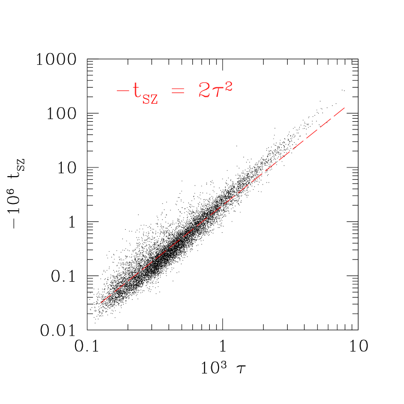
Figure 6: Scatter plot showing the height of a $t_{\rm SZ}$ peak as a function of optical depth $\tau$.

Our model for the distribution of peaks in the thermal effect is similar in spirit to that for the kinematic effect: each peak in $t_{\rm SZ}$ is associated with the centre of a dark matter halo, we ignore the effect of haloes overlapping along the line of sight. This means that we can replace the integral over the line of sight in equation (12) by an integral over the density-weighted temperature profile of the single halo of mass $m$ and concentration $c$ which happened to be in the line of sight:

$$t_{\rm SZ}(c,m) = -2r_{\rm s}\,{\sigma_{\rm T}\over m_{\rm e}}{\Omega_{\rm b}\over\Omega_{0}}\int_{0}^{W}{2w\,{\rm d}w\over W^{2}}\times$$ (13)

$$\qquad\qquad\int{\rm d}l\ {\sigma^{2}(x|c,m)\over 2c_{\rm light}^{2}}\,\rho(x|c,m),$$

where $x^{2}=l^{2}+w^{2}$, and all distances are in units of the scale radius $r_{\rm s}=r_{\rm vir}/c(m)$, with $r_{\rm vir}$ the virial radius and $c$ the concentration parameter (equation 7). As before, the integral over $w$ represents the beam smoothing. This shows that the thermal effect is proportional to the integral of the density times the internal velocity dispersion, projected along the line of sight (recall that the kinematic effect is proportional to the density times the line-of-sight bulk motion of the halo).

In principle, there is some freedom in deciding what to use for the velocity dispersion $\sigma^{2}$ within a halo. Because we are assuming, as Diaferio et al. (2000) did, that the gas and the dark matter have similar spherically symmetric density profiles with isotropic orbits, the additional assumption of hydrostatic equilibrium determines the gas velocity dispersion profile, and hence the gas temperature profile uniquely. For the Navarro et al. (1997) profile, as well as for the Hernquist (1990) profile which we discussed earlier, the velocity dispersion profile $\sigma^{2}(r)$ has a fairly complicated functional form (Hernquist 1990; Cole & Lacey 1996). Although the shape of $\sigma^{2}(r)$ is different from the circular velocity profile $Gm(<r)/2r$, the two profiles are not very different. The circular velocity profile has a much simpler functional form, and Cramphorn (2001) shows the result of setting $\sigma^{2}(r)=Gm(<r)/2r$, and then evaluating the required integral above for the Navarro et al. (1997) profile numerically. He states that the result is well approximated by $\tau^{2}\approx-t_{\rm SZ}/2$, in agreement with the simulation result in Diaferio et al.

For the Hernquist (1990) profile we discussed earlier, the integral above can be done analytically, both for the correct one-dimensional dispersion, and when the circular velocity is used to approximate the dispersion (see Appendix A). Recall that, on small scales, Hernquist’s profile has the same slope as that of Navarro et al. (1997), so we expect that using it provides a reasonable analytic approximation. The upper solid curve in Fig. 5 shows our analytic expression for the beam averaged $\sqrt{-t_{\rm SZ}}$ associated with Hernquist profiles when the squared circular velocity is used for $\sigma^{2}$, and the dashed curve shows the result of using the actual dispersion. Recall that the other curves in the Figure show the optical depth. Thus, Fig. 5 shows that both $|t_{\rm SZ}|$ and $\tau$ increase monotonically with halo mass, and that, to a good approximation, $-t_{\rm SZ}\propto\tau^{2}$. Moreover, the dashed line shows a slope slightly steeper than two at high masses, as it is indeed seen in Fig 6. The constant of proportionality is of order two, consistent with the simulations. The difference between the solid and the dashed $t_{\rm SZ}$ curves can be thought of approximately illustrating what might happen if our assumption that the gas traces the spherically symmetric dark matter distribution is relaxed.

4.2 The distribution of $\tau$ and $t_{\rm SZ}$

The previous subsection showed how to estimate the beam averaged optical depth and thermal SZ effect due to single haloes of mass $m$. If all haloes of a given mass had exactly the same density and velocity dispersion profiles, then we would be able to translate the distribution of halo masses into distributions of $\tau$ and $t_{\rm SZ}$. In fact, haloes of fixed $m$ do not all have the same profile shape: the distribution of shapes is well parametrized by assuming that the profile is always of the form given by Navarro et al. (1997), but letting the concentration parameter $c$ defined earlier follow a lognormal distribution (Jing 2000; Bullock et al. 2001). Therefore, we will assume that

$$p(t_{\rm SZ}|m)\,{\rm d}t_{\rm SZ}={{\rm d}c/c\over\sqrt{2\pi\sigma^{2}_{\rm c}}}\exp\left(-{\ln^{2}[c(t_{\rm SZ},m)/\bar{c}(m)]\over 2\sigma^{2}_{\rm c}}\right),$$ (14)

where the mean concentration at fixed mass, $\bar{c}(m)$, is given by equation (7), and the rms scatter, $\sigma_{\rm c}\approx 0.2$, is approximately independent of halo mass. The number density of the thermal effect peaks of height $t_{\rm SZ}$ is just this times the number of haloes of mass $m$, integrated over all $m$:

$$n(t_{\rm SZ})\,{\rm d}t_{\rm SZ}=\int{\rm d}m\ n(m)\,p(t_{\rm SZ}|m)\,{\rm d}t_{\rm SZ}.$$ (15)

To proceed, we need $c(t_{\rm SZ},m)$. This can be got by inverting the $t_{\rm SZ}(c,m)$ relation given above. Recall that $t_{\rm SZ}(c,m)$ can be evaluated analytically if the profile has the form given by Hernquist (1990), so that the Jacobian ${\rm d}c/{\rm d}t_{\rm SZ}$ can also be given analytically.

The number density of peaks of height $\tau$ in the optical depth distribution can be got analogously:

$$n(\tau)\,{\rm d}\tau=\int{\rm d}m\ n(m)\,p\Bigl{(}c(\tau,m)|m\Bigr{)}\,{{\rm d}c(\tau,m)\over{\rm d}\tau}\,{\rm d}\tau.$$ (16)

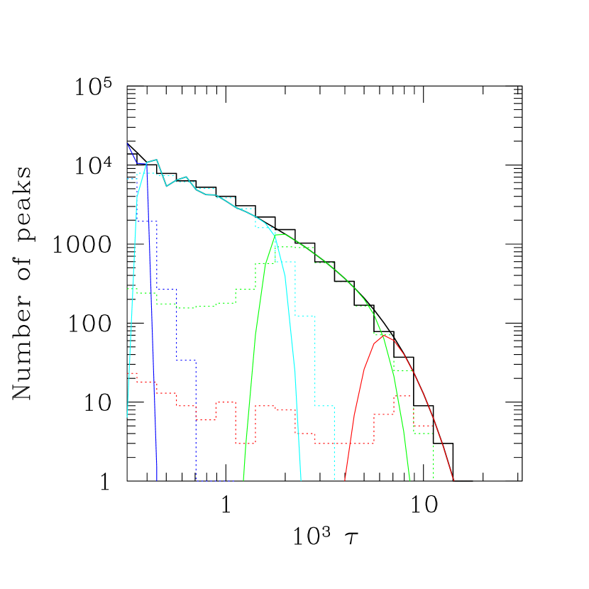
Figure 7: Distribution of optical depth peaks $\tau$ in the simulations (solid histograms) and in our model (smooth solid curves). Dashed lines show the contributions to the total from haloes with mass in the range $10^{13}$–$10^{14}$, $10^{14}$–$10^{15}$, and $\geq 10^{15}M_{\odot}/h$.

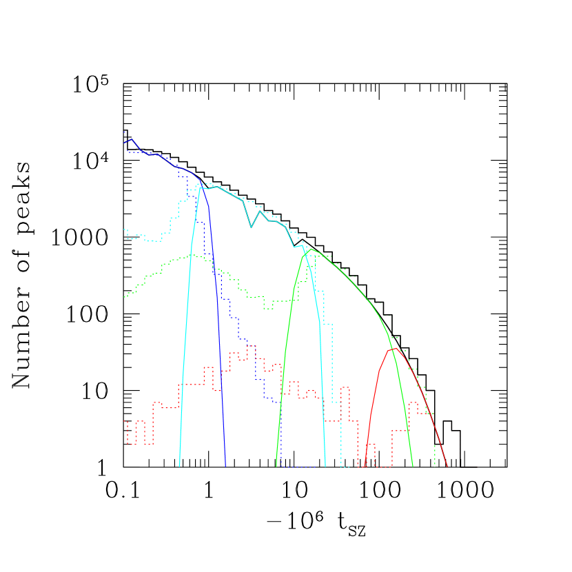
Figure 8: Distribution of peak heights $t_{\rm SZ}$ in the thermal effect in the simulations (solid histograms) and in our model (smooth solid curves). Both simulations and model assume that the gas traces the dark matter. Dashed lines show the contributions to the total from haloes with mass in the range $10^{13}$–$10^{14}$ (dominate at small $\tau$), $10^{14}$–$10^{15}$, and $\geq 10^{15}M_{\odot}/h$ (dominate at large $\tau$).

Figs. 7 and 8 show the distributions of optical depth and thermal effect peak heights in the simulations. Solid lines show the total number density of peaks, and dashed lines show the contribution to the total from haloes in small mass ranges. In the model, for the sake of simplicity, we compute $t_{\rm SZ}$ (see equation (13)) using the Hernquist profile and its corresponding circular velocity. The dashed lines were computed by locating dark matter haloes using the spherical overdensity algorithm with density threshold 200 (details are in Tormen 2001, in preparation). Simulation particles which reside in the dark matter haloes in a given mass range were marked, and then the SZ effect and Thomson optical depth were computed by using only the marked particles.

These distributions are bimodal; our model fits the large $\tau$ peak for each mass range reasonably well. This suggests that the large $\tau$ peak is due to the central cusp of a halo, whereas the increase at small $\tau$ is primarly due to the substructure of haloes which our model does not account for. Note, however, that by the time we are seeing the effect of halo-substructure, the dominant contribution to $t_{\rm SZ}$ is from the central cusps of less massive haloes.

The careful reader will have noticed that a scatter in $c$ at fixed $m$ leads to a scatter in optical depth at fixed mass $\tau(m)$. This, in turn, leads to scatter in the kinematic effect $k_{\rm SZ}$, which is in addition to the scatter induced by the fact that haloes are moving with different speeds $v$. In ignoring the scatter which is due to the distribution of halo concentrations at fixed $m$, we, in effect, assumed that the scatter in bulk velocities $v$ was the dominant cause of the scatter in $k_{\rm SZ}$ at fixed $m$, as it is indeed.

5 Discussion

We presented a simple model for the distribution of peak heights in maps of the kinematic and thermal Sunyaev-Zeldovich effects. In our model, which is similar in spirit to that proposed by Cole & Kaiser (1988), there is a one-to-one correspondence between a peak in the kinematic or the thermal effect and the presence of a massive cluster. So the shape of the distribution of peaks is determined by the mass function of clusters, and by how clusters move. If the distribution of initial density fluctuations was Gaussian, then the motions of clusters along the line of sight should be reasonably well fit by a Gaussian, so one might have expected the distribution of $k_{\rm SZ}$ peak heights to also be Gaussian. Our simulations showed that, in fact, the distribution of $k_{\rm SZ}$ peak heights is highly non-Gaussian. We argued that this happens because the kinematic effect is proportional to the product of the cluster velocity and its optical depth, the optical depths of clusters depend strongly on cluster mass, and the mass range of clusters which cause peaks in the kinematic effect is quite large. In our model, the cluster mass function and the rms motions of clusters are quantities which can be computed if the initial spectrum of density perturbations is specified. Therefore, the kinematic effect can be used to constrain the shape of this spectrum.

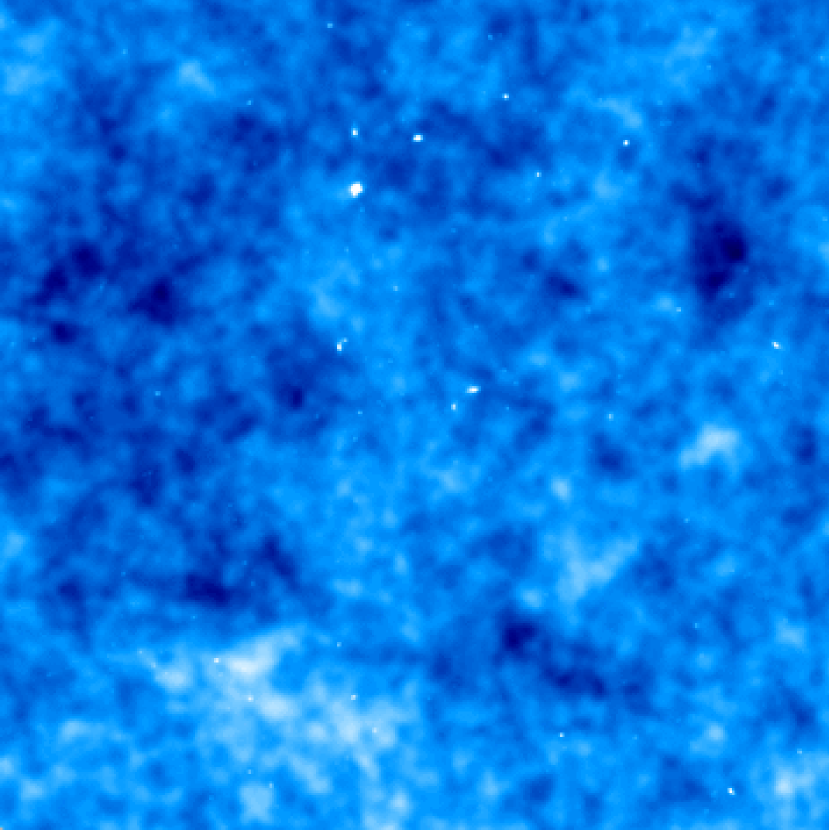
Figure 9: Distribution of temperatures in simulated 8^∘ $\times$ 8^∘ maps of the intrinsic CMB fluctuations with the thermal SZ effect fluctuations superimposed. Top panel shows the full map, and bottom panel shows what remains after applying a high-pass filter of scale one arcminute. The maps shown here are part of the full map computed from the entire 480Mpc$/h$ box.

Our model also allowed us to estimate the distribution of peak heights in the optical depth (which is not observable) and in the thermal effect (which is). To illustrate the logic, we showed what one predicts for the shapes of these non-Gaussian distributions if gas traces the dark matter. Our model was able to describe the simulations quite well. For the optical depth and for the thermal effect, the non-Gaussianity was a consequence of the non-Gaussian shape of the halo mass function. The main aim of this paper was to show how our knowledge of halo speeds and profiles can be used to model the thermal and kinematic SZ effects.

Real CMB maps will have the peaks of the SZ effects on top of the primary fluctuations. The primary fluctuations are Gaussian distributed with an rms, on arcminute scales, of about $4\times 10^{-5}$. This rms is a few times larger than the typical thermal SZ effect, and an order of magnitude larger than the typical kinematic SZ effect. However, in our $\Lambda$CDM model, the SZ effect fluctuations and the primary fluctuations dominate the angular power spectrum of the CMB on substantially different scales, which separate at $\ell\sim 3000$ (e.g. Springel, White & Hernquist 2001). Thus, in principle, an optimal high-pass filter for the arcminute scale should be able to isolate the peaks due to the SZ effects from the primary fluctuations.

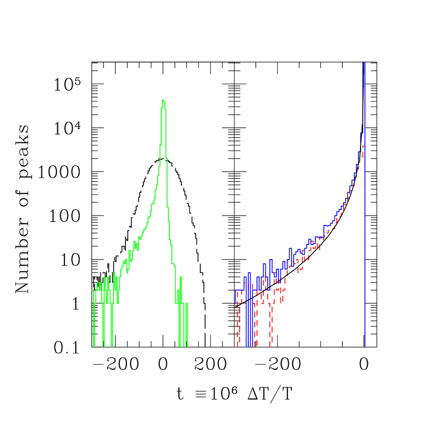
Figure 10: Distribution of peak heights in simulated temperature maps. Dashed histogram in panel on left shows the peaks in the unfiltered map shown (Fig. 9 top). Solid, slightly asymmetric histogram shows the peak heights in the high-pass filtered map (Fig. 9 bottom). Right panel compares the actual $t_{\rm SZ}$ peak decrements (solid histogram) and the peak distribution after subtracting the positive peak height distribution from the negative side in the filtered map (dashed histogram). Solid curve shows what our model predicts. The final distribution in the filtered map is similar to the actual $t_{\rm SZ}$ distribution, and is similar to what our model predicts.

If we put our simulation box at z=0.218, then the angular size of one pixel is 1 arcminute, and the whole box occupies 40^∘ $\times$ 40^∘ square-degrees. In Fig. 9, we show a small 8^∘ $\times$ 8^∘ piece of the whole map, so as to make smaller angular scale structures visible. For the analysis in Fig. 10, however, we use the entire map. The top panel in Figure 9 shows a simulated temperature map in which the $t_{\rm SZ}$ effect fluctuations are superimposed on the primary fluctuations generated at the last scattering epoch. We made a two dimensional random Gaussian field for the primary temperature fluctuations. We computed the angular power spectrum by CMBFAST for the $\Lambda$CDM model we consider here. The bottom panel shows the effect of applying a high-pass filter of scale one arcminute to this map; the large scale modulations are gone, and only small scale fluctuations remain.

Fig. 10 shows the distribution of temperature peak heights in the simulated map which has both primary and $t_{\rm SZ}$ fluctuations (dashed histogram) and in the high-pass filtered map (solid histogram); i.e., the peak height distributions in the maps shown in Fig. 9. The Gaussian-like shape of the dashed curve for the unfiltered map is primarily due to the peak height distribution of the intrinsic peaks (we have verified that it is similar to the analytic formula for peaks in two-dimensional Gaussian random fields given in Bond & Efstathiou 1987); the $t_{\rm SZ}$ peaks account for most of the large decrement tail. The solid histogram in the left panel, from the filtered map, is slightly asymmetric. If we assume that the positive peaks are due to the intrinsic CMB fluctuations, whereas the decrements are either intrinsic or $t_{\rm SZ}$ peaks, then subtracting the positive side from the negative one should leave the $t_{\rm SZ}$ peak distribution. The dashed histogram in the right panel shows what remains after doing this subtraction. It should be compared with the true distribution of $t_{\rm SZ}$ peaks which we presented earlier in the paper, and is now shown as the solid histogram. The smooth solid curve shows what our model predicts. Notice how similar the dashed and solid histograms are. This demonstrates that by suitably filtering the map, it should be possible to recover the true distribution of $t_{\rm SZ}$ peaks, and that the our model does a good job of describing this distribution.

Unfortunately, this method will not work for recovering the distribution of the $k_{\rm SZ}$ peaks. To distinguish the kinematic from the thermal effect, we must use their different spectral properties: multi-band follow-up observations of regions with deep and highly clustered $t_{\rm SZ}$ decrements will assure the presence of a supercluster where the $k_{\rm SZ}$ effect is largest (e.g. Diaferio et al. 2000).

In fact, the $t_{\rm SZ}$ peaks will also show up in clustering statistics. The shape of the correlation function of the peaks which were imprinted on the background radiation at the last scattering surface depends on peak height (Bond & Efstathiou 1987; Heavens & Sheth 1999; Heavens & Gupta 2001). The presence of $t_{\rm SZ}$ peaks will change this dependence because, as our model shows, the two-point correlation function of the SZ peaks is related to the two-point correlation function of massive clusters. Since accurate analytical models for the clustering of clusters exist (e.g. Mo & White 1996; Sheth & Tormen 1999), the clustering of the peaks in the SZ effect can be estimated rather easily, although we have not done so here. The clustering of clusters depends differently on the initial spectrum of fluctuations than the clustering of intrinsic peaks does; therefore, our model for the $t_{\rm SZ}$ peak distribution will be important if one wishes to obtain constraints on the initial fluctuation spectrum by studying the two-point and higher order moments of peaks in the microwave background on arcminute scales.

Finally, note that our model assumes that there is a one-to-one correspondence between a peak in the kinematic or thermal effects and the presence of a massive cluster. We showed that, at low redshift, this is a good approximation–our model describes the simulations quite well. At higher redshifts this assumption is likely to break down for the kinematic SZ effect. This is because, at higher redshifts, there are fewer massive haloes with sufficiently high optical depths to produce obvious peaks. In particular, the number density of massive clusters drops faster than does the typical coherent–flow speed, so that, at higher redshifts, an increasing fraction of peaks will be caused by the velocity field, rather than by the density field.

Since the kinematic peaks due to coherent flows at high redshift have a different angular structure from those due to nearby clusters, an optimal filter will be able to distinguish the two types of peaks. Developing a model for this additional effect is the subject of work in progress.

We thank Simon White, Rashid Sunyaev, Naoshi Sugiyama, Atsushi Taruya and Adi Nusser for helpful comments. This research was partly supported by the NATO Collaborative Linkage Grant PST.CLG.976902. RKS is supported by the DOE and NASA grant NAG 5-7092 at Fermilab.

Appendix A Projections of Hernquist profiles

The main text uses expressions for the density and the density-weighted temperature profiles of dark matter haloes integrated along the line of sight. For the Hernquist profile, both these integrals can be done analytically (Hernquist 1990). (Analytic results can also be obtained for many of the more general profiles in Zhao 1996; in the interests of brevity, we have not provided explicit expressions here.)

The density at $x=r/r_{\rm s}$, where $r_{\rm s}$ is a scale radius, from the centre of a Hernquist profile is

$$\rho(x)={m\,(1+b)^{2}\over 2\pi\,b^{3}r_{\rm vir}^{3}\,x(1+x)^{3}},$$ (17)

where $b=r_{\rm s}/r_{\rm vir}$ is the scale radius in units of the virial radius. Reasonable agreement with Navarro et al. (1997) profiles of the same $m$ and concentration $c$ can be got by setting $b=\sqrt{2}/c^{0.75}$ (Sheth et al. 2001).

The integral over the density, which is related to the optical depth, is

$$I(z)=\int\rho(x)\,{\rm d}l={m\,(1+b)^{2}\over 2\pi\,b^{2}r^{2}_{\rm vir}}{(2+z^{2})\,h(z)-3\over(z^{2}-1)^{2}},$$ (18)

where, in the integrand, $x^{2}=l^{2}+z^{2}$, with $x$, $l$, and $z$ all in units of the scale radius $br_{\rm vir}$, and $h(z)$ is given in the main text. This quantity, averaged over a circular window of radius $R$, is

$$2\int_{0}^{Z}{{\rm d}z\over Z}{z\over Z}\ I(z)=2\,{m\,(1+b)^{2}\over 2\pi\,b^{2}r^{2}_{\rm vir}}\,{1-h(Z)\over Z^{2}-1},$$ (19)

where $Z\equiv R/(br_{\rm vir})$.

There is some freedom as to how we should estimate the temperature. If we assume that the halo is not rotating, then the quantity of interest is the density-weighted line-of-sight velocity dispersion. If the distribution of orbits of dark matter is isotropic, and the gas moves like the dark matter, then this is

$$S(z) = {Gm\over br_{\rm vir}}\,{m\,(1+b)^{4}\over 2\pi\,b^{2}r_{\rm vir}^{2}}\,\Biggl{[}{6-65z^{2}+68z^{4}-24z^{6}\over 12(1-z^{2})^{3}}-\pi z$$ (20)

$$\qquad-{z^{2}h(z)(8z^{6}-28z^{4}+35z^{2}-20)\over 4(1-z^{2})^{3}}\Biggr{]},$$

and the average over a circle is

$$2\int_{0}^{Z}{{\rm d}z\over Z}{z\over Z}\ S(z) = 2\,{Gm\over br_{\rm vir}}\,{m\,(1+b)^{4}\over 2\pi\,b^{2}r_{\rm vir}^{2}}$$ (21)

$$\ \times\ \Biggl{[}{3-17Z^{2}+22Z^{4}-8Z^{6}\over 12(1-Z^{2})^{3}}-{\pi Z\over 3}$$

$$\ \ +\ \ \ h(Z)\,{15Z^{2}-20Z^{4}+8Z^{6}\over 12(1-Z^{2})^{2}}\Biggr{]}.$$

If, instead, we use one half of the circular velocity squared,

$${v_{\rm c}^{2}\over 2}\equiv{Gm(<r)\over 2r}={Gm\,(1+b)^{2}\over 2\,br_{\rm vir}}{x\over(1+x)^{2}},$$ (22)

then we need

$$V(z)=\int{v_{\rm c}^{2}(x)\over 2}\,\rho(x)\,{\rm d}l={Gm\over br_{\rm vir}}\,{m\,(1+b)^{4}\over 2\pi\,b^{2}r_{\rm vir}^{2}}\,{h_{2}(z)/2\over(z^{2}-1)^{4}},$$ (23)

where

$$h_{2}(z)={6+83z^{2}+16z^{4}\over 12}-{5z^{2}\,(4+3z^{2})\over 4}\,h(z).$$

This, averaged over a circle of radius $Z$ is

$$2\int_{0}^{Z}\!{{\rm d}z\over Z}{z\over Z}\ \!V(z)\! = \!{Gm\over br_{\rm vir}}\,{m\,(1+b)^{4}\over 2\pi\,b^{2}r_{\rm vir}^{2}}\times$$ (24)

$$\Biggl{[} \!\!\!\!\!\!{-3-14Z^{2}+2Z^{4}\over 12(Z^{2}-1)^{3}}+{15Z^{2}\,h(Z)\over 12(Z^{2}-1)^{3}}\Biggr{]}.$$

References

- [1] Bond J. R., Efstathiou G. P., 1987, MNRAS, 226, 655
- [2] Bullock J. S., et al., 2001, MNRAS, 321, 559
- [3] Cole S., Kaiser N., 1988, 233, 637
- [4] Cole S., Lacey C., 1996, MNRAS, 281, 716
- [5] Cramphorn C., 2001, Astronomy Letters, 27, 135
- [6] da Silva A. C., Barbosa D., Liddle A. R., Thomas P. A., 2000, MNRAS, submitted (astro-ph/0011187)
- [7] Diaferio A., Sunyaev R. A., Nusser A., 2000, ApJL, 533, L71
- [8] Heavens A. F., Sheth R. K., 1999, MNRAS, 310, 1062
- [9] Heavens A. F., Gupta S., 2001, MNRAS, submitted, astro-ph/0010126
- [10] Hernquist L., 1990, ApJ, 356, 359
- [11] Jing Y. P., 2000, ApJ, 535, 30
- [12] Mo H. J., White S. D. M., 1996, MNRAS, 282, 347
- [13] Navarro J., Frenk C. S., White S. D. M., 1997, ApJ, 490, 493
- [14] Peebles P. J. E., Juszkiewicz R., 1998, ApJ, 509, 483
- [15] Refrigier A., Teyssier R., 2000, preprint astro-ph/0012086
- [16] Seljak U., Zaldarriaga M., 1996, ApJ, 469, 437
- [17] Seljak U., Burwell J., & Pen U.-L., 2001, PRD, 630, 619
- [18] Sheth R. K., Tormen G., 1999, MNRAS, 308, 119
- [19] Sheth R. K., Diaferio A., 2001, MNRAS, 322, 901
- [20] Sheth R. K., Hui, L., Diaferio A., & Scoccimarro, R., 2001, MNRAS, in press
- [21] Springel V., White M., Hernquist L., 2001, ApJ, 549, 681
- [22] Sunyaev R. A., Zel’dovich Ya., 1980, MNRAS, 190, 413
- [23] Tormen G., 2001, in preparation
- [24] Zhao H., 1996, MNRAS, 278, 488