*

Abstract

An overview is given of Bayesian inversion and regularization procedures. In particular, the conceptual basis of the maximum entropy method (MEM) is discussed, and extensions to positive/negative and complex data are highlighted. Other deconvolution methods are also discussed within the Bayesian context, focusing mainly on the comparison of Wiener filtering, Massive Inference and the Pixon method, using examples from both astronomical and non-astronomical applications.

1 Introduction

In the next few years there will exist all-sky datasets from two new satellite missions for the Cosmic Microwave Background (the MAP and Planck missions), along with very large datasets from optical surveys such as 2dF and Sloan. The combined effect of these new data on quantitative cosmology will be enormous, but at the same time pose great problems in terms of the scale of data analysis effort required.

As an example, the Planck Surveyor satellite, due for launch in 2007, combines both HEMT and bolometer technology in 10 frequency channels covering the range 30 GHz to 850 GHz, with a highest angular resolution of 5 arcmin. An artist’s impression of this satellite is shown in Figure 1,

Figure 1: Artist’s impression of the Planck Satellite

and the experimental parameters of the Planck mission are summarized in Table 1.

Table 1: Approximate experimental parameters of the Planck satellite. HFI refers to the high frequency part of the instrument, and LFI is the low frequency instrument. The $\Delta T/T$ sensitivity is per beam area in one year (thermodynamic temperature)

	LFI (HEMT)				HFI (Bolometers)
$\nu$ GHz	30	44	70	100	100	143	217	353	545	857
No. of detectors	4	6	12	34	4	12	12	6	8	6
$\theta_{\rm FWHM}$	$33^{\prime}$	$23^{\prime}$	$14^{\prime}$	$10^{\prime}$	$10.7^{\prime}$	$8^{\prime}$	$5.5^{\prime}$	$5^{\prime}$	$5^{\prime}$	$5^{\prime}$
$\Delta T/T\times 10^{-6}$	1.6	2.4	3.6	4.3	1.7	2.0	4.3	14.4	147	6670
Polarization	yes	yes	yes	yes	no	yes	yes	yes	no	no

The mission is designed to give high sensitivity to CMB structures, together with sufficient frequency coverage to enable accurate separation of the non-CMB physical components. These will typically be Galactic dust, synchrotron and free-free emission, together with extragalatic radio and sub-mm/FIR sources. Also present will be the effects of Sunyaev-Zeldovich distortion of the CMB as it passes through the hot intracluster gas of clusters of galaxies. This separation of components must be performed using data from approximately 100 detectors in total, spanning ten frequencies, and with the sky map at each frequency containing on the order of $10^{7}$ pixels. These figures give some idea of the scale of the problem, for just this mission alone, and suggest why the idea of ‘mining the sky’ is appropriate.

The task of analysing modern large datasets is undeniably challenging in terms of the amount of data to be processed. In the pursuit of ‘precision cosmology’, however, we are faced with the additional requirement that the data must be analysed in a statistically rigorous way. In CMB observations, for example, one is interested in the statistical properties of CMB anisotropies, most commonly summarised by their power spectrum $C_{\ell}$, from which it is possible to derive estimates and confidence limits on fundamental cosmological parameters such as the matter density of the Universe or the value of the cosmological constant. Similar statistical measures are central to the analysis of optical surveys. Thus, in modern cosmology, one is faced with the dual problem of analysing large datasets while retaining statistical rigour. In the present paper, we discuss both aspects, particularly in the context of how an efficient choice of ‘basis functions’ can lead to both an improved analysis and large speed-up factors.

It is now generally accepted that the correct way to draw inferences from any set of data is to apply Bayes’ theorem in a consistent and logical manner. This provides a general framework in which the analysis of CMB and optical survey data can be performed. Let us consider the generic problem at hand. In order to recover an underlying signal $s$ from some measured data $d$, we commonly need to solve an inverse problem such as

$$\mbox{\boldmath$d$}=R\mbox{\boldmath$s$}+\mbox{\boldmath$\epsilon$},$$ (1)

where $R$ represents the response matrix of the experiment and $\epsilon$ is the instrumental noise vector. For simplicity, we are assuming here that the inversion problem is linear, although this is not strictly necessary. In any case, owing to the presence of noise, the properties of which are only known statistically (sometimes even this is not true), the inversion problem is degenerate. Even in absence of noise, a direct inversion would, in general, not be possible, since the response matrix $R$ is normally not invertible. For instance, $R$ may be a blurring (beam) function, which strongly suppresses higher spatial frequencies, or it may represent a beam-differencing experiment where some spatial frequencies are actually set to zero. Thus, it is clear that some kind of statistical technique is needed in order to regularise the inversion. This naturally leads us to a Bayesian approach. This is one of the most powerful current techniques of image reconstruction.

In the present paper, we discuss different deconvolution methods within the Bayesian framework, showing that different techniques are actually obtained by different choices of priors and/or basis functions. The outline of the paper is as follows. §2 gives an introduction to Bayes’ theorem and derives the Wiener filter in this context. §3 describes the Maximum Entropy Method (MEM), including extensions to positive/negative and complex data, and discusses some applications. The Pixon Method is introduced in §4. §5 discusses multiscale and wavelet MEM. The Massive Inference technique is introduced in §6. Finally, conclusions are given in §7.

2 Mining the Sky with Bayes’ Theorem

Let us recall the original problem

$$\mbox{\boldmath$d$}=R\mbox{\boldmath$s$}+\mbox{\boldmath$\epsilon$},$$ (2)

For simplicity we assume $\langle\mbox{\boldmath$s$}\rangle=\mbox{\boldmath$0$}=\langle\mbox{\boldmath$\epsilon$}\rangle$

To obtain the ‘best’ sky reconstruction we chose to maximise the probability $Pr(\mbox{\boldmath$s$}|\mbox{\boldmath$d$})$ using Bayes’ theorem

$$Pr(\mbox{\boldmath$s$}|\mbox{\boldmath$d$})=\frac{1}{Pr(\mbox{\boldmath$d$})}\,Pr(\mbox{\boldmath$d$}|\mbox{\boldmath$s$})\,Pr(\mbox{\boldmath$s$}),$$ (3)

where $Pr(\mbox{\boldmath$s$}|\mbox{\boldmath$d$})$ is the posterior probability of an underlying signal (or true sky) $s$ given some data $d$, $Pr(\mbox{\boldmath$d$}|\mbox{\boldmath$s$})$ is the likelihood funtion and $P(\mbox{\boldmath$s$})$ is the prior probability. At the first level of Bayesian inference $Pr(\mbox{\boldmath$d$})$, the evidence, is merely a normalisation, which implies we wish to maximise

$$Pr(\mbox{\boldmath$s$}|\mbox{\boldmath$d$})\propto Pr(\mbox{\boldmath$d$}|\mbox{\boldmath$s$})\,Pr(\mbox{\boldmath$s$})$$ (4)

For convenience we consider the case of Gaussian noise, although this is not necessary (for instance there exist many applications to Poisson noise). For Gaussian noise, the likelihood is simply

$$Pr(\mbox{\boldmath$d$}|\mbox{\boldmath$s$})\propto\,\mathrm{e}^{\mbox{\footnotesize$-{\textstyle\frac{1}{2}}\mbox{\boldmath$\epsilon$}^{T}N^{-1}\mbox{\boldmath$\epsilon$}$}}\,=\,\mathrm{e}^{\mbox{\footnotesize$-{\textstyle\frac{1}{2}}(\mbox{\boldmath$d$}-R\mbox{\boldmath$s$})^{T}N^{-1}(\mbox{\boldmath$d$}-R\mbox{\boldmath$s$})$}}\,$$ (5)

where $N=\langle\mbox{\boldmath$\epsilon$}\mbox{\boldmath$\epsilon$}^{T}\rangle$ is the noise covariance matrix. This is usually written as $Pr(\mbox{\boldmath$d$}|\mbox{\boldmath$s$})\propto\exp(-{\textstyle\frac{1}{2}}\chi^{2})$. Now we have to decide on the assignment of the prior, $Pr(\mbox{\boldmath$s$})$. As a first approach, we assume that $s$ (which, for a CMB experiment, for example, would include CMB anisotropies, the Sunyaev-Zeldovich effect, Galactic emission, etc.) is a Gaussian random variable, described by a known covariance matrix $C=\langle\mbox{\boldmath$s$}\mbox{\boldmath$s$}^{T}\rangle$ (including all cross-correlations) so that

$$Pr(\mbox{\boldmath$s$})\propto\,\mathrm{e}^{\mbox{\footnotesize$-{\textstyle\frac{1}{2}}\mbox{\boldmath$s$}^{T}C^{-1}\mbox{\boldmath$s$}$}}\,$$ (6)

In this case the posterior probability is

$$Pr(\mbox{\boldmath$s$}|\mbox{\boldmath$d$})\propto Pr(\mbox{\boldmath$d$}|\mbox{\boldmath$s$})\,Pr(\mbox{\boldmath$s$})\propto\,\mathrm{e}^{\mbox{\footnotesize$-{\textstyle\frac{1}{2}}(\chi^{2}+\mbox{\boldmath$s$}^{T}C^{-1}\mbox{\boldmath$s$})$}}\,$$ (7)

which one must maximise with respect to $s$ to obtain the reconstruction. This is equivalent to minimising $F={\textstyle\frac{1}{2}}(\chi^{2}+\mbox{\boldmath$s$}^{T}C^{-1}\mbox{\boldmath$s$})$. In fact, we can do better than this. By completing the square in $s$ (e.g. [1]), we can recover the whole posterior distribution:

$$Pr(\mbox{\boldmath$s$}|\mbox{\boldmath$d$})\propto\,\mathrm{e}^{\mbox{\footnotesize$-{\textstyle\frac{1}{2}}(\mbox{\boldmath$s$}-\hat{\mbox{\boldmath$s$}})^{T}E^{-1}(\mbox{\boldmath$s$}-\hat{\mbox{\boldmath$s$}})$}}\,$$ (8)

where the sky reconstruction $\hat{\mbox{\boldmath$s$}}$ is given by

$$\hat{\mbox{\boldmath$s$}} = W\mbox{\boldmath$d$},$$ (9)

$$W = (C^{-1}+R^{T}N^{-1}R)^{-1}R^{T}N^{-1},$$ (10)

where $W$ is in fact the Wiener matrix and

$$E=(C^{-1}+R^{T}N^{-1}R)^{-1}$$ (11)

is the reconstruction error matrix $E=\langle(\mbox{\boldmath$s$}-\hat{\mbox{\boldmath$s$}})(\mbox{\boldmath$s$}-\hat{\mbox{\boldmath$s$}})^{T}\rangle$. Thus we have recovered the optimal linear method, which is usually derived by minimising residual variances.

We recall that in general the response matrix $R$ will not be invertible. However, it is remarkable that the estimation of the sky $\hat{\mbox{\boldmath$s$}}=W\mbox{\boldmath$d$}$ can still be computed no matter how singular $R$ is, since it only needs $R^{T}$ to be evaluated. This is an example of regularization. Notice how if the $C^{-1}$ were not present in $W$ we would just have $W=R^{-1}$. We say that we have regularized the inverse.

The above solution is ‘easy’ to calculate and has known reconstruction errors. It is, however, by no means the best solution in real problems. For instance, consider the standard ‘Lena’ IEEE test image in Fig. 2. The original image (top left panel) is smoothed with a Gaussian blurring function with a FWHM of 6 pixels followed by the addition of noise (top right panel). The Wiener filter reconstructed image is given in the bottom right panel. Although some improvement is achieved, spurious structure (‘ringing’) appears at small scales. For comparison, a result generated using a pixon method (see §4) is also shown.

Figure 2: Comparison of the performance of a pixon method to the Wiener filter for the ‘Lena’ test image. The original image has been blurred with a Gaussian blurring function with a FWHM of 6 pixels followed by addition of noise

3 The Maximum Entropy Method

The main shortcoming of the Wiener filter is that relies on the assumption of Gaussianity and the a priori knowledge of the covariance matrix. Real data, however, is rarely so simple, and we must therefore consider alternative priors. A possible choice is the entropy prior (Maximum Entropy Method, MEM).

Usually MEM is applied to positive, additive distibutions (PADS). Let $h$ be the (true) pixel vector we are trying to estimate. In this case very general considerations of subset independence, coordinate invariance and system independence lead uniquely to the prior $Pr(\mbox{\boldmath$h$})\propto\,\mathrm{e}^{\mbox{\footnotesize$\alpha S$}}\,$ where the ‘entropy’ $S$ ([2]) of the image is given by

$$S(\mbox{\boldmath$h$},\mbox{\boldmath$m$})=\sum_{i}\left(h_{i}-m_{i}-h_{i}\ln\left(\frac{h_{i}}{m_{i}}\right)\right)$$ (12)

where $m$ is the measure on an image space (the model) to which the image $h$ defaults in the absence of data (it can be shown that the global maximum of $S$ occurs at $\mbox{\boldmath$h$}=\mbox{\boldmath$m$}$). In fact, it has been shown recently ([3]) that, if there exist linear constraints on the signal (e.g. like $\mbox{\boldmath$d$}=R\mbox{\boldmath$s$}+\mbox{\boldmath$\epsilon$}$ in our case), the form of the entropic prior is determined uniquely by simply requiring consistency with the sum and product rules of probability.

‘Subset independence’ implies, however, that no a priori correlations between the pixels of $h$ should be present. So, is it possible to include known covariance structure, as in the Wiener method?. The answer is yes!. Given a sky $s$ with $C=\langle\mbox{\boldmath$s$}\mbox{\boldmath$s$}^{T}\rangle$, we form the Cholesky decomposition

$$C=LL^{T}$$ (13)

where $L$ is an upper triangular matrix, and define a hidden, uncorrelated i.i.d. (independent, identically distributed) unit variance hidden field $h$ related to $s$ by

$$\mbox{\boldmath$s$}=L\mbox{\boldmath$h$}$$ (14)

It is straightforward to show that, with this construction, $\langle\mbox{\boldmath$s$}\mbox{\boldmath$s$}^{T}\rangle=C$. Thus the derivation of $S(\mbox{\boldmath$h$},\mbox{\boldmath$m$})$ applies to this hidden variable and we need to maximise

$$Pr(\mbox{\boldmath$h$}|\mbox{\boldmath$d$}) \propto \,\mathrm{e}^{\mbox{\footnotesize$-{\textstyle\frac{1}{2}}\chi^{2}(\mbox{\boldmath$h$})+\alpha S(\mbox{\boldmath$h$},\mbox{\boldmath$m$})$}}\,$$ (15)

$${\rm where}~{}~{}~{}\chi^{2}(\mbox{\boldmath$h$}) = (\mbox{\boldmath$d$}-RL\mbox{\boldmath$h$})^{T}N^{-1}(\mbox{\boldmath$d$}-RL\mbox{\boldmath$h$})$$ (16)

The vector $\hat{\mbox{\boldmath$h$}}$ that maximises this expression is the MEM reconstruction. Note that $\alpha$ is a regularising parameter of the relative weight of the data and the prior. Large $\alpha$ favours large entropy (i.e., $\hat{\mbox{\boldmath$h$}}$ close to $m$) at expense of the data, whereas small $\alpha$ gives more weight to the data. The parameter $\alpha$ can be estimated itself via Bayesian methods ([2]). Crudely, the value of $\alpha$ is such that

$$\chi^{2}(\hat{\mbox{\boldmath$h$}})\approx N,$$ (17)

where $N$ is the number of good degrees of freedom in the data. Note that for $\alpha=0$, the method reduces to maximum likelihood. For $\alpha=2$ and small $h_{i}$ (in fact for $h_{i}\mathrel{\hbox to0.0pt{\lower 3.5pt\hbox{$\mathchar 536\relax$}\hss}\raise 1.5pt\hbox{$\mathchar 316\relax$}}3m,\forall_{i}$) it can be shown that the method is Wiener filter again ([4]). This means that the Wiener filter is simply a quadratic approximation of MEM with $\alpha=2$.

Another important issue is how to calculate the errors on the reconstruction. This is performed by making a Gaussian approximation to the posterior probability distribution $Pr(\mbox{\boldmath$h$}|\mbox{\boldmath$d$})$ at its peak $\hat{\mbox{\boldmath$h$}}$. Moreover, by sampling from this distribution within, say, the $1\sigma$ surface, one can generate sample reconstructions all compatible with the data, which can be very informative.

An interesting application of MEM to astronomical data is the recovery of the projected mass density of a galaxy cluster from observations of its gravitational lensing effects on background galaxies ([5]). This technique is particularly interesting since it directly maps the dark matter halos in clusters. Moreover, together with the projected mass distribution, an estimation of errors is also obtained. Figure 3 shows the projected mass density of the cluster MS1054 reconstructed from shear data obtained by [6] using the Hubble Space Telescope.

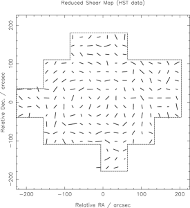
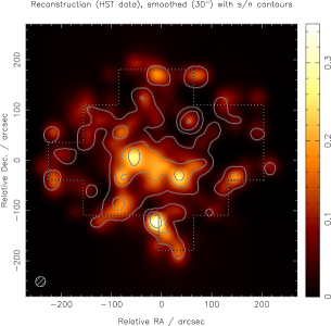
Figure 3: The shear field in the direction of the galaxy cluster MS1054, determined from HST observations, and the corresponding MEM reconstruction of the projected mass density in the cluster (courtesy of Phil Marshall)

A further extension of MEM is necessary in order to apply the algorithm to positive and negative data (such as CMB) and also to complex data (e.g. Fourier transforms). Indeed, it is possible to generalise MEM to both of these kinds of data. For a positive and negative image, we just need to write $h$ as the difference between two positive images

$$\mbox{\boldmath$h$}=\mbox{\boldmath$u$}-\mbox{\boldmath$v$}$$ (18)

Applying continuity constraints, we then obtain the entropic prior for positive/negative images as

$$S(\mbox{\boldmath$h$},\mbox{\boldmath$m$}) = \sum_{i}\psi_{i}-2m_{i}-h_{i}\ln\left(\frac{\psi_{i}+h_{i}}{2m_{i}}\right)$$ (19)

$${\rm with~{}~{}}\psi_{i} = \sqrt{h_{i}^{2}+4m_{i}^{2}}.$$ (20)

The posterior probability is given, as before, by $\exp(-{\textstyle\frac{1}{2}}\chi^{2}+\alpha S)$, but now using this generalised definition of entropy. This result can be derived directly from counting arguments (‘monkeys throwing balls’) [7]. Regarding complex images, we can just treat real and imaginary parts separately:

$$S(\mbox{\boldmath$h$},\mbox{\boldmath$m$})=S(\Re(\mbox{\boldmath$h$}),\Re(\mbox{\boldmath$m$}))+S(\Im(\mbox{\boldmath$h$}),\Im(\mbox{\boldmath$m$}))$$ (21)

where $\Re$ and $\Im$ denote the real and imaginary parts of each vector. This generalisation to positive/negative and complex images is actually a key point, since MEM now can be applied to the Fourier Transform (or Spherical Transform for the all-sky case) of the original maps or images. But in Fourier space, modes at different $k$ (or $l,m$ on a sphere) can generally be treated independently, therefore we can apply MEM separately at each mode. This means that we have $N_{pix}$ minimisations with respect to one or a few variables, instead of a single minimisation with respect to $N_{pix}$ variables. This leads to a huge speed-up in the algorithm, which is crucial for large data sets.

We call this FastMEM or FourierMEM. This method has been successfully applied to reconstructing the different components of the microwave sky from simulated Planck data of small patches of the sky ([4]). An application of FastMEM to Planck data is also given in this volume ([8]). Moreover, an extension of the algorithm to deal with all-sky data, which works in spherical harmonic space, is currently being tested ([9]).

Figure 4: Results of MEM as applied to Planck simulated data on the whole sky. From top to bottom the maps correspond to input CMB, input dust and residuals for the MEM reconstructed CMB (from [9])

Fig. 4 shows the performance of this technique for simulated all-sky Planck data. The input CMB and Galactic dust maps are shown, but in addition the simulations also contain Galactic synchrotron and free-free emission as well as thermal and kinetic Sunyaev-Zeldovich effect from clusters of galaxies. The bottom panel shows the residuals in the MEM reconstruction of the CMB. It is striking that, even when no cut of the Galactic plane has been attempted, no obvious emission from the Galaxy has contaminated the reconstructed CMB, except for a few pixels in the centre of the map.

FastMEM has also performed very well in non-astronomical data. The left panel of Fig. 5 shows the blurred image (due to the instrument response) of a pollen grain obtained by combining 20 images taken at different depths with a confocal microscope. The reconstructed image achieved by FastMEM is shown in the right panel. The amount of detail recovered with respect to the original image is very noticiable. Besides, FastMEM takes around 45 seconds to perform such a reconstruction versus 50 minutes needed by real spece MEM.

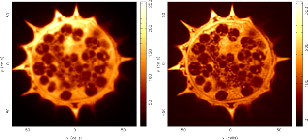
Figure 5: Blurred image of a pollen grain and FastMEM reconstruction

4 The Pixon Method

A recent addition to the stable of image reconstruction algorithms is the pixon method ([10]). The basic idea behind this technique is to minimise the number of degrees of freedom used to describe an image while still maintaining an acceptable fit to the data. This is achieved by, instead of working in the pixel basis, describing the image using ‘pixons’, which are essentially flexible pixels able to change shape and size. For example, in the pixon approach, only a few large pixons are needed to describe the background or parts of the image with a low signal to noise ratio, whereas a larger number of smaller pixons are used where the signal has more detail.

The pixon idea can in fact be phrased within in the framework of Bayes’ theorem via the introduction of a prior. Let there be $N$ counts (e.g. photons) in total that must be assigned to $n$ cells (or pixons) and assume $N_{i}$ counts end up in pixon $i$ , so $\sum_{i}N_{i}=N$. Thus, we need to choose $n$ and $N_{i}$ and also the position of the pixons in the least informative way. The total number of possibilities is given by $n^{N}$. The total number having a given $N_{1}$ in pixon $1$, $N_{2}$ in pixon $2$, etc. is $\frac{N!}{\Pi_{i}N_{i}!}$. So, the probability of a given arrangement is

$$Pr({\rm arrangement})=\frac{N!}{n^{N}\Pi_{i}N_{i}!}$$ (22)

Note that this probability favours arrangements with a small number of pixons containing a large number of counts instead of having a large number of cells with only few counts. Indeed, it is maximised by $n=1$ and $N_{i}=N$. So, we can use this probability as a prior combined with the likelihood term to obtain the posterior probability. Moreover, using Stirling’s approximation, we can write this as

$$Pr({\rm arrangement})\approx\frac{1}{n^{N}}\exp\left(-\sum_{i}\frac{N_{i}}{N}\ln\frac{N_{i}}{N}\right)$$ (23)

which is similar to an entropy prior. Thus, the pixon method can be seen as a MEM that allows ‘pixel sizes’ (and shapes) to vary as well.

Note that we have described the ‘pure form’ of the pixon method, but so far the commercial code has had to include a large number of modifications relative to this in order to get an algorithm that works properly and rapidly enough. An independent implementation of the Pixon method for cluster detection is given by [11] in this volume. Indeed, the notion of distinct ‘hard-edged’ pixons of different shapes and sizes is unhelpful in the reconstruction of general images, and current pixon algorithms tend to favour a ‘fuzzy-pixon’ approach, which is equivalent simply to the assumption of an instrinsic correlation length for the structure in the image, which can vary across the image. Thus, the reconstructed image $I$ is written as the local convolution of a pseudo-image $I_{\rm pseudo}$ with a pixon shape function $K$, whose width varies over the image

$$I(\mbox{\boldmath$x$}_{i})=\int_{V_{\mbox{\boldmath$y$}}}K\left(\frac{\mbox{\boldmath$y$}-\mbox{\boldmath$x$}_{i}}{\delta_{i}}\right)I_{\rm pseudo}(\mbox{\boldmath$y$})dV_{\mbox{\boldmath$y$}},$$ (24)

where $\mbox{\boldmath$x$}_{i}$ is the location of pixel $i$ and $\delta_{i}$ is the pixon size at pixel $i$. The pixon shape can be arbitrary (which can be a strength or a weakness of the method in different circumstances). A common choice is a truncated inverted paraboloid ([12]), which leads to (except for a normalisation)

$$K=\left\{\begin{array}[]{ll}1-\frac{|\mbox{\boldmath$y$}-\mbox{\boldmath$x$}_{i}|^{2}}{\delta_{i}^{2}},&|\mbox{\boldmath$y$}-\mbox{\boldmath$x$}_{i}|\leq\delta_{i}\\ 0,&|\mbox{\boldmath$y$}-\mbox{\boldmath$x$}_{i}|>\delta_{i}\\ \end{array}\right.$$ (25)

The basic algorithm is very simple. Firstly, some initial choice is made for the pixon width $\delta_{i}$ in each pixel. Often this can be simply $\delta_{i}=1$ for all $i$, but this can lead to ‘freezing-in’ of unwanted small-scale structure, so in some cases the $\delta_{i}$ are chosen to be somewhat larger. In any case, given the initial choice of the $\delta_{i}$ the maximum-likelihood solution for the pseudo-image $I$ is obtained in a standard manner. Then, keeping this pseudo-image fixed, the pixon widths $\delta_{i}$ are varied until a set is found where each $\delta_{i}$ has the largest possible value that is still consistent with the data in a least-squares sense. This whole two-step process is then repeated until convergence is achieved.

Figure 6: Comparison of the performance of the Pixon method to traditional MEM. Top row (from left to right): original image, blurred and noisy image, Pixon reconstructed image, MEM reconstruction. Centre row: surface plots for the images in top raw. Bottom row: blurring function, additive noise, residuals for Pixon Method, residuals for MEM. (Images from http://casswww.ucsd.edu/personal/puetter/pixonpage.html)

Fig. 2 showed a comparison between the pixon method and the Wiener filter. We see that the pixon method clearly outperforms Wiener filter. Another example is given in Fig. 6. In this case, a synthetic image composed of a sharp peak and a valley is used to compare the pixon method and MEM. The image has been blurred and Gaussian noise added. We see that the recovery of the peak and valley are similar for both Pixon and MEM, but the low level noise present in the background of the MEM reconstruction has been successfully removed in the Pixon image. In addition, the residuals for the Pixon method seem compatible with random noise whereas MEM produces residuals correlated with the signal.

5 Multiscale and wavelet MEM

Although the reconstructions in Figure 6 show the pixon method to be very effective, the comparison is not strictly reasonable, since it employs the traditional MEM technique, which is rarely still used in this simple form.

It has long been realised that the key to effective image reconstruction is to reduce the number of degrees of freedom one is trying to constrain. The simplest way of achieving this goal is via the assumptions of an intrinsic correlation length that does not vary across the image ([13]); this was discussed briefly in §3. Basically, one hypothesises the existence of a hidden space $h$ that is linearly-related to the signal space $s$ by an intrinsic correlation function $L$, such that

$$\mbox{\boldmath$s$}=L\mbox{\boldmath$h$}.$$ (26)

One then performs the MEM reconstruction in terms of $h$ (which is a priori uncorrelated). The corresponding signal reconstruction $s$ will thus have an intrinsic correlation length determined by $L$ and hence fewer independent degrees of freedom. This clearly corresponds to the pixon method with all the pixon widths $\delta_{i}$ being equal.

However, this simple method can be greatly enhanced by choosing $L$ in a more innovate way. The most obvious extension is to allow for the existence of multiple hidden fields, each related to signal space by convolutions of different widths. This then reproduces the ability to have varying effective correlation lengths across the image, but in a such way that the the correlation length at each point in the image is determined via a proper entropic regularisation of the hidden fields, and not by an arbitrary least-squares criterion as is done in the pixon method. Application of this ‘multiscale MEM’ technique to numerous types of images has shown it to be very successful. An interesting astronomical example is again provided by gravitational lensing. Figure 7 shows the reconstruction of the projected mass density in the cluster MS1054 from the shear data shown in Figure 3.

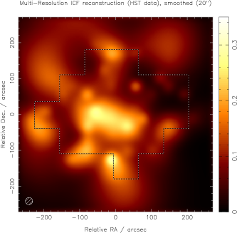
Figure 7: The multiscale MEM reconstruction of the projected mass density in the cluster MS1054 (courtesy of Phil Marshall)

In this case, however, the reconstruction has been performed using a 4-level multiscale MEM algorithm. By comparing with the traditional MEM reconstruction in Figure 3 one sees that the small scale rippling has disappeared, and indeed the calculated evidence for the 4-scale reconstruction is much higher. By way of illustration, in Figure 8 we also plot the corresponding hidden fields that constitute the reconstruction.

Figure 8: The hidden fields that constitute the multiscale MEM reconstruction in Figure 7 of MS1054 (courtesy of Charlie McLachlan)

One can see from figure 8 that the mutliscale MEM approach is equivalent to providing a set of (redundant, non-orthogonal) basis functions for the image that are simply the different intrinsic correlation functions. The MEM is simply obtaining a properly regularised optimal solution for the values of the coefficients of each basis function required to reconstruct the image. Once viewed in this way, one may wonder if there exist more efficient sets of basis functions one could use to describe the image. Clearly, the number of degrees of freedom is simply equal to the number of basis functions required, and so one wishes to find a basis in which general images can be described with relatively few basis functions. The obvious choice is wavelets. These functions are constructed so that they are well-localised in both position and frequency space, and have proven to be very effective in representing an image with few basis functions (their extensive use in image compression is also obviously a result of this property). Indeed, by using a wavelet transform kernel to relate the spaces $h$ and $s$, the reconstruction quality can be improved still further.

6 Massive Inference

Massive Inference ([14],[15]) can be seen as an even more extreme choice of basis functions. In this method, we throw away the underlying pixelisation grid and instead represent the object as a variable number of ‘atoms’ or ‘point masses’. Each of these is described by a position $\mbox{\boldmath$x$}_{j}$ and a flux $z_{j}$. To simulate a continuum, $\mbox{\boldmath$x$}_{j}$ runs over $2^{32}$ positions. We need to assign a prior probablity to $x$ and $z$ as well as to the number of atoms $N$.

Each of the $N$ locations is assigned a uniform prior, i.e., $Pr(\mbox{\boldmath$x$}_{i})=\mbox{constant}$. The number of atoms can be assigned a Poisson distribution with a given mean $\alpha$:

$$Pr(N)=\frac{\,\mathrm{e}^{\mbox{\footnotesize$-\alpha$}}\,\alpha^{N}}{N!}$$ (27)

Finally, each of the $N$ amplitudes is assigned an exponential prior (with parameter $q$):

$$Pr(z_{i})=\frac{\,\mathrm{e}^{\mbox{\footnotesize$-z_{i}/q$}}\,}{q}$$ (28)

The program (using Markov Chain Monte Carlo sampling and simulated annealing) then samples the posterior probability (which also includes the likelihood term) treating $\alpha$ and $q$ as hyperparameters.

So far, some spectacular results have been obtained for 1-dimensional spectra and 2-dimensional point sources. An early application of Massive Inference has been to flash photolysis data for proteins in corn grains, including a comparison with MEM. Figure 9 shows simulations of the decay of luminescence measured in the experiment. The important question is how many decaying exponentials are present in these data, and what are their decay rates.

Figure 9: The decay of luminescence in a simulated flash photolysis experiment

In Figure 10 the results obtained using MassInf and MEM are given.

Figure 10: The decaying exponential components present in Figure 9 as determined by MassInf (left) and MEM (right) respectively

We see that MassInf is far more successful in determining a narrow range of possible decay rates. Most importantly, the MassInf algorithm can also provide the probability distribution for the number of distinct exponential components, as shown in Figure 11.

Figure 11: The probability distribution for the number of distinct decaying exponential components, as determined by MassInf

Table 2 summarises the similarities and differences between MEM and Massive Inference.

Table 2: Comparison between of MEM and Massive Inference

MEM	MassInf
Pixel based	Continuum
Gradient Search	Markov Chain Monte Carlo
Needs differential $\underline{R}(a)$	Transform $R(f)$ only
and adjoint $\overline{R}(a)$
Poisson errors OK	$\chi^{2}$ only
Multi-dimensional	One-dimensional
	(needs Peano curve)
Gaussian approximation	Direct sampling
Fast global transforms OK	Slow atom transforms
Computing time $\propto$ grid size	Computing time $\propto$ number atoms

7 Conclusions

We have seen that a Bayesian approach provides a common statistical framework for several important methods currently used in astronomical processing and analysis. By generalising one’s view to include also the optimal choice of basis functions it is clear how significant improvements can be obtained both in the quality of the resulting reconstructions and in the speed at which the analysis can be carried out. These two aspects will both be crucial in the new era of quantitative cosmology which is now opening up.

Acknowledgments

We would like to thank Vlad Stolyarov, Sarah Bridle, Phil Marshall and Charlie McLachlan for help with several of the figures and Steve Gull for the simulations shown in Figures 9–11.

References

- [1] Zaroubi S., Hoffman Y., Fisher K.B., Lahav O., 1995, ApJ, 449, 446
- [2] Skilling J., 1989, in ‘Maximum Entropy and Bayesian Methods’, J.Skilling (ed), Kluwer Academic Publishers, Dordtrecht, p. 45
- [3] Garrett A., 2000, ‘Maximum Entropy from the Laws of Probability’, in ‘Maximum Entropy and Bayesian Methods’, Paris, ed. Mohammad-Djafari A., AIP.
- [4] Hobson M.P., Jones A.W., Lasenby A.N., Bouchet F.R., 1998, MNRAS, 300, 1
- [5] Bridle S.L., Hobson M.P., Lasenby A.N., Saunders R., 1998, MNRAS, 299, 895
- [6] Hoekstra H., Franx M., Kuijken K., 2000, ApJ, 532, 88
- [7] Hobson M.P., Lasenby A.N., 1998, MNRAS, 298, 905
- [8] Barreiro R.B., Vielva P., Hobson M.P., Martínez-González E., Lasenby A.N., Sanz J.L., Toffolatti L., in this volume
- [9] Stolyarov V. et al., in preparation
- [10] Piña R.K., Puetter R.C., 1993, PASP, 105, 630
- [11] Eke V., in this volume
- [12] Puetter R.C., 1994, SPIE Vol.2302 Image Reconstruction and Restoration, 112
- [13] Gull S.F., 1989, in ‘Maximum Entropy and Bayesian Methods’, J.Skilling (ed), Kluwer Academic Publishers, Dordtrecht, p. 53
- [14] Skilling J., 1998, in ‘Maximum Entropy and Bayesian Methods’, G.Erickson, J.T.Rychert, C.Ray.Smith (eds), Kluwer Academic Publishers, Dordtrecht, p. 14
- [15] Skilling J., 1999, MassInf Programmers’ Notes. Maximum Entropy Data Consultants Ltd, Royston