The discriminating power of wavelets to detect non-Gaussianity in the CMB

Abstract

We investigate the power of wavelet techniques in detecting non-Gaussianity in the cosmic microwave background (CMB). We use the method to discriminate between an inflationary and a cosmic strings model using small simulated patches of the sky. We show the importance of the choice of a good test statistic in order to optimise the discriminating power of the wavelet technique. In particular, we construct the Fisher discriminant function, which combines all the information available in the different wavelet scales. We also compare the performance of different decomposition schemes and wavelet bases. For our case, we find that the Mallat and à trous algorithms are superior to the 2D-tensor wavelets. Using this technique, the inflationary and strings models are clearly distinguished even in the presence of a superposed Gaussian component with twice the rms amplitude of the original cosmic string map.

1 Introduction

The Cosmic Microwave Background (CMB) is currently one of the most powerful tools of cosmology to investigate the theories of structure formation in the Universe. In particular, the standard inflationary model predicts Gaussian fluctuations whereas alternative theories such as topological defects scenarios give rise to non-Gaussianity in the temperature field. Therefore, the study of the Gaussian character of the CMB will allow us to discriminate between these two competitive theories of structure formation. In addition, future high-resolution maps should be investigated for any trace of non-Gaussianity that may be imprinted by foregrounds or systematics.

In order to test the Gaussianity of the CMB, a large number of methods have been proposed (for a review see Barreiro 2000). Perhaps the most straightforward of these is the measurement of the skewness and kurtosis of the distribution of the pixel temperatures in the map (Scaramella & Vittorio 1991). More complex methods include properties of hot and cold spots (Coles & Barrow 1987; Martínez-González et al. 2000; Barreiro, Martínez-González & Sanz 2001), extrema correlation function (Naselsky & Novikov 1995, Kogut et al. 1996, Barreiro et al. 1998, Heavens & Sheth 1999), Minkowski functionals (Coles 1988, Gott et al. 1990, Kogut et al. 1996), bispectrum analysis (Ferreira et al. 1998, Heavens 1998, Magueijo 2000), multifractals (Pompilio et al. 1995) and partition function (Diego et al. 1999, Martínez-González et al. 2000).

In addition, tests of Gaussianity based on wavelets have become quite popular in the last years. Ferreira, Magueijo & Silk (1997) propose a set of statistics using cumulants and defined in wavelet space. Hobson, Jones & Lasenby (1998) investigate the power of the cumulants of the distribution of wavelet coefficients at each scale on detecting the Kaiser-Stebbins effect using CMB simulations of small patches of the sky. A similar method was introduced by Forni & Aghanim (1999) and tested using simulated CMB maps containing secondary anisotropies (Aghanim & Forni 1999) and on the COBE data (Aghanim, Forni & Bouchet 2001). Pando, Valls-Gabaud & Fang (1998) calculated the skewness, kurtosis and scale-scale correlation coefficients of the COBE data in the QuadCube pixelisation using planar orthogonal wavelets. This study was extended by Mukherjee et al (2000). Barreiro et al (2000) applied the same method to the COBE data in HEALPix pixelisation using spherical wavelets.

This paper is an extension of the work done by Hobson et al (1998) (HJL, hereinafter). As in HJL, the fourth cumulant of the distribution of wavelet coefficients is calculated at each wavelet scale using high-resolution CMB simulations of small patches of the sky for Gaussian and non-Gaussian simulations. However, in this work, all this information is combined into the Fisher discriminant function in order to get a more statistically significant result. In addition, we compare the performance of three different ways of constructing 2-dimensional wavelets: tensor (as in HJL), Mallat and the à trous algorithm. Moreover, some of the studied wavelets are invariant under rotations of 90, 180 and 270 degrees of the original data, which solves the earlier problem of orientation sensitivity.

The outline of the paper is as follows. §2 gives a brief introduction to the three different constructions of 2-dimensional wavelets. In §3 our non-Gaussianity test is explained in detail, also pointing out the interest of the Fisher discriminant function. The results of applying this test to simulated data are given in §4. Finally, our conclusions are presented in §5.

2 The discrete wavelet transform

The wavelet transform has been extensively discussed elsewhere (e.g. Daubechies 1992). In particular, a clear introduction to wavelets is given by Burrus, Gopinath & Guo (1998). We therefore give only a brief introduction, pointing out the differences between the three considered decomposition schemes. The basis of the wavelet transform is to decompose the considered signal (the temperature field in our case) into a set of wavelet coefficients. Each of them contain information about the signal at a given position and scale. Therefore, wavelets allow one to study the structure of an image at different scales and at the same time keep localisation. There is not a unique choice for a wavelet basis. Moreover, different algorithms schemes can be used to construct 2-dimensional wavelets. In particular, we consider the tensor, Mallat (or multiresolution) and à trous algorithms.

2.1 Tensor algorithm

This is the type of wavelets used in the analysis of HJL, where a more detailed description can be found. In 1-dimension, the wavelet basis is constructed from dilations and translations of the mother (or analysing) wavelet function $\psi$ and a second related function called the father (or scaling) wavelet function:

$$\psi_{j,l} = 2^{\frac{j-J}{2}}\psi\left(2^{j-J}x-l\right)\,,$$

$$\phi_{j,l} = 2^{\frac{j-J}{2}}\phi\left(2^{j-J}x-l\right)\,,$$ (1)

where $0\geqslant j\geqslant J-1$ and $0\geqslant l\geqslant 2^{J}-1$ are integer denoting the dilation and translation indices, respectively, and $2^{J}$ is the number of pixels of the considered discrete signal $f(x)$.

In order to construct a real, orthogonal and compactly-supported wavelet basis, such as the Haar and Daubechies 4 wavelets used in this work, these functions must satisfy some highly-restrictive mathematical relations (Daubechies 1992). The discrete signal $f(x)$ can thus be written as

$$f(x_{i})=a_{0,0}\phi_{0,0}(x_{i})+\sum_{j}\sum_{l}d_{j,l}\psi_{j,l}(x_{i})\,,$$ (2)

being $a$, $d$ the approximation and detail wavelet coefficients respectively. These coefficients can be found in a recursive way starting from the data vector $f(x_{l})\equiv a_{J,l},l=0,..,2^{J}-1$

$$a_{j-1,l} = \sum_{m}h(m-2l)a_{j,m}$$

$$d_{j-1,l} = \sum_{m}g(m-2l)a_{j,m}\,.$$ (3)

where $h$, $g$ are the low and high-pass filters associated to the scaling and wavelet functions through the refinement equation (see e.g. Burrus et al. 1998). At each iteration, the vector of length $2^{j}$ is split into $2^{j-1}$ detail components and $2^{j-1}$ smoothed components. The decimated smoothed components are then used as input for the next iteration to construct the detail coefficients at the next larger scale. This produces a number of wavelet coefficients equal to the original number of pixels. As the index $j$ increases from 0 to $J-1$, the wavelet coefficients correspond to the structure of the function on increasingly smaller scales, with each scale a factor of 2 finer than the previous one.

The extension of the DWT to 2-dimensional signals is obtained by taking tensor products of the one-dimension wavelet basis as follows

$$\phi_{0,0;l_{1},l_{2}}(x,y) = \phi_{0,l_{1}}(x)\phi_{0,l_{2}}(y)$$

$$\zeta_{j_{1},0;l_{1},l_{2}}(x,y) = \psi_{j_{1},l_{1}}(x)\phi_{0,l_{2}}(y)$$

$$\xi_{0,j_{2};l_{1},l_{2}}(x,y) = \phi_{0,l_{1}}(x)\psi_{j_{2},l_{2}}(y)$$

$$\psi_{j_{1},j_{2};l_{1},l_{2}}(x,y) = \psi_{j_{1},l_{1}}(x)\psi_{j_{2},l_{2}}(y).$$

If the two-dimensional pixelised image has dimensions $2^{J}\times 2^{J}$ then we have $0\leqslant j_{1}\leqslant J-1$ and $0\leqslant l_{1}\leqslant 2^{j_{1}}-1$, and similarly for $j_{2}$ and $l_{2}$.

With this wavelet decomposition scheme, the wavelet transform is performed independently in both directions. By analogy with the one-dimensional case, as $j_{1}$ ($j_{2}$) increases the wavelet coefficients contain information about the horizontal (vertical) structure in the image on increasingly smaller scales. In particular, the scale corresponding to each region is approximately $\sim$pixel size$\times 2^{J-j_{i}}$ in each direction. Therefore, regions with $j_{1}=j_{2}$ contain coefficients of two-dimensional wavelets that represent the image at the same scale in the horizontal and vertical directions. Conversely, domains with $j_{1}\neq j_{2}$ contain wavelet coefficients describing the image on different scales in the two directions.

2.2 Mallat algorithm

For the previous wavelets, the wavelet transform is applied separately for each direction of the image. This means that some of the domains contain mixing of structure with different scales $j_{1}$ and $j_{2}$ in the horizontal and vertical directions. However, it is possible to use one-dimensional bases to construct two-dimensional bases that do not mix scales and can be described in terms of a single scale index $j$ (Mallat 1989). At scale $j$, these bases are given by

$$\phi_{j;l_{1},l_{2}}(x,y) = \phi_{j,l_{1}}(x)\phi_{j,l_{2}}(y)$$

$$\psi^{\rm H}_{j;l_{1},l_{2}}(x,y) = \psi_{j,l_{1}}(x)\phi_{j,l_{2}}(y)$$

$$\psi^{\rm V}_{j;l_{1},l_{2}}(x,y) = \phi_{j,l_{1}}(x)\psi_{j,l_{2}}(y)$$

$$\psi^{\rm D}_{j;l_{1},l_{2}}(x,y) = \psi_{j,l_{1}}(x)\psi_{j,l_{2}}(y).$$

In this wavelet decomposition, the temperature map (scale $J$) is decomposed into an approximation image (that is basically a lower resolution version of the original image) plus three details images. These detail coefficients contain horizontal, vertical and diagonal structure at scale $J-1$ that encode the differences between the original and lower resolution images. The same decomposition is applied then to the approximation image, generating a lower resolution image and another three details at scale $J-2$. This process is repeated down to the lowest resolution level considered. The scale of the structure contained by a wavelet coefficient with index $j$ correspond approximately to pixel size$\times 2^{J-j}$ As for the tensor case, the wavelet basis is non-redundant and orthogonal. Thus, the number of wavelet coefficients is the same as the number of pixels. We also note that the diagonal wavelet coefficients obtained with the Mallat algorithm are the same as those with $j_{1}=j_{2}$ in the tensor decomposition.

Although different orthogonal wavelet bases were tested for the tensor and Mallat algorithms, we present our results for Haar and Daubechies 4 (see §4). We note that it is not possible to construct a real orthogonal wavelet basis with compact support whose wavelet basis functions are also symmetric. Therefore the wavelet transform will not be invariant under rotations. However, the Haar wavelet functions are antisymmetric. This means that our test will be invariant under rotations of 90, 180 and 270 degrees of the data with respect to the original orientation when using the Haar wavelets basis.

2.3 À trous algorithm

The à trous (‘with holes’) algorithm (Holschneider & Tchamitchian 1990; Shensa 1992) is a redundant non-orthogonal wavelet transform. Given a data vector $f(x_{l})\equiv c_{J,l},l=0,...,2^{J}-1$, the approximation coefficients for the next lower resolution are obtained as

$$a_{j-1,l}=\sum_{m}h(m)a_{j,l+2^{(J-j)}m}$$ (4)

i.e., each step is a convolution of the data with the filter $h$ and varying step sizes $2^{J-j}$. The function $h$ is a discrete low pass filter associated to a scaling function $\phi(x)$ that can be derived from a refinement relation (see e.g. Starck & Murtagh 1994). The corresponding detail coefficients are simply obtained by subtracting the smoother image from the original one:

$$d_{j-1,i}=a_{j,k}-a_{j-1,k},$$ (5)

Since no decimation is carried out between consecutive filter steps, the number of wavelet coefficients at each scale is $2^{J}$. Note that the reconstruction of the signal is particularly simple in this case, obtained by adding the detail wavelet coefficients at all scales plus the approximation coefficients at the lowest considered resolution:

$$c_{J,l}=c_{0,l}+\sum_{j=0}^{J-1}w_{j,l}$$ (6)

We have chosen a $B_{3}$-spline for the scaling function, which leads to a convolution with a mask $(\frac{1}{16},\frac{1}{4},\frac{3}{8},\frac{1}{4},\frac{1}{16})$ in 1-dimension and

$$\left(\begin{array}[]{ccccc}\frac{1}{256}&\frac{1}{64}&\frac{3}{128}&\frac{1}{64}&\frac{1}{256}\\ \frac{1}{64}&\frac{1}{16}&\frac{3}{32}&\frac{1}{16}&\frac{1}{64}\\ \frac{3}{128}&\frac{3}{32}&\frac{9}{64}&\frac{3}{32}&\frac{3}{128}\\ \frac{1}{64}&\frac{1}{16}&\frac{3}{32}&\frac{1}{16}&\frac{1}{64}\\ \frac{1}{256}&\frac{1}{64}&\frac{3}{128}&\frac{1}{64}&\frac{1}{256}\\ \end{array}\right)$$ (7)

in 2-dimensions (e.g. Starck & Murtagh 1994). Note that, due to the symmetry of the mask, the à trous wavelet transform is invariant under rotations of the data of 90, 180 and 270 degrees with respect to the original orientation.

3 The non-Gaussianity test

The non-Gaussianity test used in this paper is basically the same as that of HJL. The main idea is to perform a wavelet transform of the (possibly) non-Gaussian image and obtain certain statistic of the wavelet coefficients in each region of the transform. In particular, we estimate the fourth cumulant $\hat{\kappa}_{4}$ for each scale. This quantity is calculated using $k-$statistics as explained in HJL. We repeat this test for a large number (10000) of non-Gaussian and Gaussian realisations and then compare the distribution of the fourth cumulant spectra $\hat{\kappa}_{4}(r)$ obtained from the two different populations. This is different to HJL where only a single non-Gaussian map was used to test the power of the wavelet technique (see §4). Each Gaussian map is obtained from one of the non-Gaussian maps by randomising its phases. Therefore, Gaussian and non-Gaussian maps share the same power spectrum by construction. This is important to ensure that any possible differences found between both populations are due to the non-Gaussian character of the test map rather than differences in the power spectrum.

As discussed in HJL, due to edge effects, not all wavelet coefficients can be used in the analysis. We need to discard those coefficients obtained from wavelet functions that cross the boundary of the image to avoid misidentifying these borders as non-Gaussian features. To identify the affected wavelet coefficients, we perform a wavelet transform of a map consisting of zeroes except for a border of non-zero pixels on the map boundary. The resulting non-null wavelet coefficients correspond to edge-crossing basis functions and are therefore ignored in the subsequent analysis.

One can, of course, repeat the test using cumulants other than $\kappa_{4}$. We have obtained results for $\kappa_{3}$, but find it to be a less discriminating statistic than in the case studied here.

3.1 The discriminating power of a test

In HJL, the significance of the test was given by the level of the highest detection of non-Gaussianity. However, a single detection of non-Gaussianity may not be statistically significant if all the other estimators are consistent with a Gaussian distribution. Conversely, when the level of confusion is high, it may happen that no single statistic detects non-Gaussianity at a high significance level. Nevertheless, if we use all the available statistics together, we may find a systematic displacement with respect to the Gaussian distribution, which would allow us to discriminate between both models. Therefore, a more statistically rigorous analysis should take into account all the information provided by the different regions of the wavelet transform. In order to do this, we need to construct a test statistic that maximises the discriminating power between the two models.

Suppose that given a set of $n$ measurements ${\mathbf{x}}=(x_{1},...,x_{n})$, we want to check the validity of a hypothesis $H_{0}$, usually called the null hypothesis, against an alternative hypothesis $H_{1}$. Each hypothesis specifies a joint probability $f({\mathbf{x}}|H_{0})$ and $f({\mathbf{x}}|H_{1})$ for obtaining the particular values of our data. In our case, the measurements correspond to the value of the fourth cumulant at each wavelet scale and we want to test if our sample is drawn from a Gaussian model or from a cosmic strings scenario. In order to compare the level of agreement between the measured data and the considered hypotheses, it is useful to construct a function of the measured variables called a test statistic $t({\mathbf{x})}$. In principle, this statistic can be a multidimensional vector, but we consider only the case when $t$ is a scalar, since this greatly simplifies the problem by reducing the number of dimensions of the data whilst keeping enough information to discriminate between the considered hypotheses. The probability of obtaining a certain value of $t$ will be given by $g(t|H_{0})$ if $H_{0}$ is true and by $g(t|H_{1})$ if the correct hypothesis is $H_{1}$.

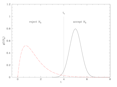
Figure 1: An example of the discriminating power of a test between two hypotheses $H_{0}$ and $H_{1}$. The solid line corresponds to the probability $g(t|H_{0})$ of obtaining a certain value of $t$ if $H_{0}$ is true, whereas the dashed line gives the same probability $g(t|H_{1})$ if $H_{1}$ is the correct hypothesis.

In order to reject or accept the hypothesis $H_{0}$, one can define a critical value for $t$ (see Fig. 1). The critical value $t_{c}$ is defined so that the probability of observing $t$ under the assumption of the hypothesis $H_{0}$ is less than a certain value $\alpha$, which is called the significance level of the test. In the example of Fig. 1 this would be given by

$$\alpha=\int_{-\infty}^{t_{\rm c}}g(t|H_{0})dt~{}.$$ (8)

Thus, there is a probability $\alpha$ of rejecting $H_{0}$ when it is actually true. This is called an error of the first kind. An error of the second kind occurs when $t$ falls in the acceptance region but it was actually drawn from an alternative hypothesis $H_{1}$. In our example, in Fig. 1, the probability of such an error happening is given by

$$\beta=\int_{t_{\rm c}}^{\infty}g(t|H_{1})dt~{}.$$ (9)

The quantity $p\equiv 1-\beta$ is called the power of the test to discriminate against the alternative hypothesis $H_{1}$ at the considered significance level. In our wavelet analysis, we will compare the values of $p$ for a significance level of $\alpha=0.01$ for each of the studied cases.

3.2 The $\chi^{2}$ test

The key issue now is the choice of a test statistic. One possibility is to uncorrelate the variables and then obtain a standard $\chi^{2}$ statistic. The procedure is as follows. First, the empirical covariance matrix $V$ of the variables is obtained from a large number of Gaussian simulations. Then, a new set of variables ${\mathbf{x}}$ is constructed by a rotation:

$${\mathbf{x}^{\prime}}=S^{T}{\mathbf{x}}$$ (10)

where $S$ is a matrix whose columns are the normalised eigenvectors of the covariance matrix $V$. The same rotation is then applied to the non-Gaussian variables. Finally, the $\chi^{2}$ statistic is obtained for each Gaussian and non-Gaussian realisation by calculating

$$\chi^{2}=\sum_{i}\left(\frac{x^{\prime}_{i}-\mu^{\prime}_{i}}{\sigma^{\prime}_{i}}\right)^{2}$$ (11)

where $x^{\prime}_{i}$ corresponds to the $i$th (Gaussian or non-Gaussian) rotated variable, and $\sigma^{\prime}_{i}$ and $\mu^{\prime}_{i}$ to the dispersion and mean value of the $i$th uncorrelated variable for the Gaussian distribution.

This method is actually equivalent to perform a generalised $\chi^{2}$ (such as that in Barreiro, Martínez-González & Sanz 2001) from the original correlated variables that takes into account the correlations between them. However, our procedure has some advantages. By uncorrelating the Gaussian variables, we can have some insight into the significance of the single detections of non-Gaussianity. In addition, it gives us the possibility of investigating a further test statistic as follows. We can construct the probability density function $P(x_{i}^{\prime})$ for each of the uncorrelated variables obtained from a large number of Gaussian simulations. Although the requirement that the variables are uncorrelated does not imply that they are independent (i.e. that their joint probability is separable), we may still construct the test statistic

$$\eta^{2}=\sum_{i}\ln\left[P(x_{i}^{\prime})\right]~{}.$$ (12)

If the joint probability of ${\mathbf{x}^{\prime}}$ is a multidimensional Gaussian, $\eta^{2}$ is equivalent to the $\chi^{2}$ (they coincide except for an additive constant and a scaling factor). The construction of a non-Gaussian $\chi^{2}$ was already introduced by Ferreira, Magueijo & Górksi (1998) to study the normalised bispectrum of the COBE data. Their definition includes some extra factors to ensure that $\eta^{2}$ defaults exactly to the standard $\chi^{2}$ when the considered variables follow a multivariate Gaussian distribution.

Unfortunately, we could not estimate this quantity for our non-Gaussian realisations. This is due to the fact that some of the values of the variables in the non-Gaussian case lie far beyond a few $\sigma$’s with respect to the distribution of the Gaussian population. This makes it very difficult to evaluate the quantity $\eta^{2}$ for the non-Gaussian distribution. Instead, we compute the standard $\chi^{2}$ statistic (11) and compare its performance to the test described below.

3.3 The Fisher discriminant function

In the previous tests, we are comparing the level of agreement of a set of data with some theoretical model. Therefore only information about this model is included in the test. However, if we believe that our data are most likely drawn either from a hypothesis $H_{0}$ or from an alternative one $H_{1}$, it is well known that an optimal test statistic in the sense of maximum power for a given significance level is given by

$$t({\mathbf{x}})=\frac{f({\mathbf{x}}|H_{0})}{f({\mathbf{x}}|H_{1})}$$ (13)

which is called the likelihood ratio (Brandt 1992). Unfortunately, in order to construct this statistic, we need to know the joint probabilities $f({\mathbf{x}}|H_{0})$ and $f({\mathbf{x}}|H_{1})$, which are in general not available.

A simpler possibility is to construct a test statistic using the Fisher linear discriminant function (Fisher 1936). This is the optimal linear function of the measured variables for separating the probabilities $g({\mathbf{t}}|H_{0})$ and $g({\mathbf{t}}|H_{1})$ in the sense of maximum distance between the expected mean values of $t$ for each model and minimum dispersion of each of them. The test statistic is given by

$$t({\mathbf{x}})=\sum_{i=1}^{n}a_{i}x_{i}={\mathbf{a}}^{T}{\mathbf{x}}$$ (14)

with

$${\mathbf{a}} \propto W^{-1}(\mu_{0}-\mu_{1})$$

$$W_{ij} = (V_{0}+V_{1})_{ij}$$ (15)

where $\mu_{k}$ and $V_{k}$ are the expected mean value and covariance matrix of the measured data if drawn from the hypothesis $H_{k}$. Thus $t({\mathbf{x}})$ is determined up to an additive constant and a scaling factor.

Actually if $f({\mathbf{x}}|H_{0})$ and $f({\mathbf{x}}|H_{1})$ are both multivariate Gaussian with common covariance matrices, the Fisher discriminant function coincides with the likelihood ratio (Cowan 1998).

In our case, the set of variables ${\mathbf{x}}$ are the fourth cumulant of the wavelet coefficients at each scale, whereas the hypotheses $H_{0}$ and $H_{1}$ correspond to our simulated data being drawn from a Gaussian and a non-Gaussian population respectively (see §4). In order to estimate the power of our non-Gaussianity test, we construct and compare the Fisher discriminant function $t$ for each Gaussian and non-Gaussian realisation. The mean values and covariance matrices of our variables for both models needed to generate the $W$ matrix are estimated from a large number of simulations.

4 Application to simulated data

In this section, we apply the wavelet analysis described above to the detection of non-Gaussianity in simulated CMB maps. As our test map, we use the same realisation of CMB anisotropies as in HJL. This is a simulated CMB map due to the Kaiser-Stebbins effect from cosmic strings (Kaiser & Stebbins 1984). The size of the simulation is $6.4\times 6.4$ deg² with a total of 256$\times$256 pixels of size 1.5 arcminutes.

In order to test the power of our non-Gaussianity test, we add to the cosmic strings map a Gaussian component that shares the same power spectrum as the test map. The weight of the Gaussian component is controlled by a parameter $b$, that gives the ratio of the non-Gaussian to Gaussian proportions as 1:$b$. We investigate which is the maximum level of this Gaussian component (i.e., the largest value of $b$) that can be introduced and still detect the underlying non-Gaussianity.

To make more realistic simulations, the test map is convolved with a Gaussian beam of FHWM=5 arcminutes. Finally, Gaussian white noise is added with an rms level equal to one-tenth that of the convolved map. This degree of smoothing and level of noise is typical of what may be achieved from CMB observations by the Planck satellite of ESA after foreground removal is performed using the Maximum-Entropy method (Hobson et al 1998).

As pointed out in the previous section, a single non-Gaussian map was used to test the power of the wavelet analysis in HJL. However, even for the same underlying non-Gaussian map, the particular value of our statistics depends on the specific Gaussian component and noise realisation that are being used. Therefore, the conclusions derived from our test will vary from one Gaussian realisation to other. To take this into account, we have analysed a large number (10000) of non-Gaussian test maps that contain the same cosmic strings map but different Gaussian component and noise realisations. Ideally, each non-Gaussian map would also contain a different cosmic strings realisation. Unfortunately, strings maps are difficult to simulate and very computationally expensive. Therefore, a large number of stringy maps are not currently available to us and we account only for the dispersion introduced by the Gaussian components of the map. Nonetheless, although the particular level of discrimination achieved by the test may vary for a different choice of a cosmic strings map, we expect the general conclusions of this work to remain valid.

Another important point is the choice of the type of wavelet and the wavelet basis. We compare the performance of three different ways of constructing wavelets: tensor, Mallat and à trous algorithm. For the tensor and Mallat algorithms, we also consider different wavelet bases. In HJL, an entropy criterion was used for finding the wavelet basis that gives the single highest detection of non-Gaussianity at a particular scale. In this paper, however, we perform a joint analysis of the information provided by all the scales and therefore we cannot apply the same criterion. We have tried Haar, Daubechies 4,6,12 and 20, Coiflet 2 and 3 and Symmlet 6 and 8 wavelet bases and find that, using the full analysis, most of them lead to similar results. In particular, more complex wavelets (such as Daubechies 12 and 20) tend to discriminate between the models slightly worse, probably because of a larger number of wavelet coefficients being discarded due to edge effects. Therefore, we present our results for Daubechies 4 and Haar wavelets since these are two of the simplest and also best known orthogonal wavelet bases. Moreover, the Haar basis functions are antisymmetric and the results of our statistic are therefore invariant under rotations of the data (by 90, 180 and 270 degrees).

4.1 Tensor algorithm

2D-tensor wavelets are constructed in the manner explained in §2.1. These are the type of wavelets used in the original work of HJL. In this section we present the results for this type of wavelets for the Daubechies 4 and Haar wavelet bases. We also show the discriminating power of the Fisher discriminant function versus a $\chi^{2}$ analysis and address the orientation sensitivity problem.

4.1.1 Daubechies 4

Figure 2: Top panel shows the fourth cumulant spectra obtained from 10000 Gaussian and non-Gaussian simulations for $b=0$, using tensor Daubechies 4 wavelets. The corresponding uncorrelated variables are given in the middle panel. The bottom panel shows the histogram of the Fisher discriminant obtained from the Gaussian (solid line) and non-Gaussian (dashed line) simulations (see text for details).

The top panel of Fig. 2 shows the fourth cumulant spectrum for the test map with non-Gaussian:Gaussian proportions (1:0) using Daubechies 4 and the original orientation of the data. Solid squares and open circles correspond to the non-Gaussian and Gaussian values respectively. The Gaussian values have been normalised to zero mean value and unit dispersion to allow for a straightforward reading in units of the Gaussian dispersion of the distance between the two models. The error bars show the 68, 95 and 99 per cent confidence levels of the Gaussian and non-Gaussian distributions derived from 10000 simulations in each case. The scale corresponding to the region number is given in Table 1; a higher region number corresponds, in general, to smaller scales. We see that there are several large detections of non-Gaussianity, the highest single detection being $\sim 60\sigma$ in region 20. This corresponds to scales of a few arcminutes ($\simeq 6-12^{\prime}$) which is expected since the characteristic signature of the Kaiser-Stebbins effect shows at small scales. As an illustration, we also show in the middle panel the corresponding rotated uncorrelated variables. These are obtained as explained in §3.2.

Table 1: Correspondence of region number with scale for tensor wavelets. The scale is calculated as $1.5^{\prime}(2^{J-j_{1}}\times 2^{J-j_{2}})$, where $2^{J}\times 2^{J}$ is the total number of pixels in the map. The fifth and sixth columns give the total number of coefficients in the region and how many of those coefficients are used to calculate the fourth cumulant of their distribution when using Daubechies 4. For the Haar wavelet, there is not need of correction for boundary effects and all coefficients are used. Finally, the last column indicates the number of the corresponding region for Mallat wavelets, for those regions that are common for both types of wavelets. For symmetry, wavelet coefficients in domains with $j_{2}>j_{1}$ are included in the same region as those with scales $(j_{2},j_{1})$. Following HJL, wavelet coefficients with $j_{i}=0$ are not included in the analysis.

region	$j_{1}$	$j_{2}$	$\sim$scale(′)	no.coeff.	used (D4)	Mallat
1	1	1	$192\times 192$	4	0	3
2	2	1	$96\times 192$	16	0
3	2	2	$96\times 96$	16	0	6
4	3	1	$48\times 192$	32	0
5	3	2	$48\times 96$	64	10
6	3	3	$48\times 48$	64	25	9
7	4	1	$24\times 192$	64	0
8	4	2	$24\times 96$	128	26
9	4	3	$24\times 48$	256	130
10	4	4	$24\times 24$	256	169	12
11	5	1	$12\times 192$	128	0
12	5	2	$12\times 96$	256	58
13	5	3	$12\times 48$	512	290
14	5	4	$12\times 24$	1024	754
15	5	5	$12\times 12$	1024	841	15
16	6	1	$6\times 192$	256	0
17	6	2	$6\times 96$	512	122
18	6	3	$6\times 48$	1024	610
19	6	4	$6\times 24$	2048	1586
20	6	5	$6\times 12$	4096	3538
21	6	6	$6\times 6$	4096	3721	18
22	7	1	$3\times 192$	512	0
23	7	2	$3\times 96$	1024	252
24	7	3	$3\times 48$	2048	1260
25	7	4	$3\times 24$	4096	3276
26	7	5	$3\times 12$	8192	7308
27	7	6	$3\times 6$	16384	15372
28	7	7	$3\times 3$	16384	15876	21

Table 2: Discriminating power of the non-Gaussianity test for different wavelets

	Tensor			Mallat			À trous
	Daubechies 4		Haar	Daubechies 4		Haar
	$0^{\circ}$	$180^{\circ}$		$0^{\circ}$	$180^{\circ}$
$b=0$	1.00	1.00	1.00	1.00	1.00	1.00	1.00
$b=1$	1.00	1.00	1.00	1.00	1.00	1.00	1.00
$b=2$	0.517	0.798	0.619	0.974	0.996	0.995	0.991
$b=3$	0.038	0.091	0.037	0.165	0.330	0.252	0.187

To evaluate in a more quantitative way the discriminating power of our non-Gaussianity test, we have obtained the Fisher discriminant function $t$ as explained in § 3.3. This is shown in the bottom panel of Fig. 2. The solid and dashed lines correspond to the histogram of $t$ for the Gaussian and non-Gaussian simulations respectively. As expected from the difference in the fourth cumulant spectrum, the curves are clearly separated. Indeed the power of the test to discriminate between both models at the 0.01 significance level is 1.

Figure 3: Fourth cumulant spectra and Fisher discriminant for $b$=1,2,3 using the tensor Daubechies 4 wavelet. Open circles/solid lines and solid squares/dashed lines correspond to the Gaussian and non-Gaussian models respectively.

In order to assess the amount of Gaussian confusion that can be added to our test map and still detect the underlying non-Gaussianity, we increase the value of $b$ until the models cannot be separated. Fig. 3 shows the fourth cumulant spectrum and Fisher discriminant function for $b=1,2,3$. For non-Gaussian:Gaussian proportions of 1:1, the presence of the non-Gaussian signature is still clear at region 20, although the level of the detection has fallen appreciably. This translates into much closer histograms for the Fisher discriminant function but the power of the test at the 0.01 significance level remains 1. When the level of Gaussian confusion is increased to $b=2$, the fourth cumulant spectrum of both models shows no clear detections. Although some differences are seen in the estimated mean values of both populations, the error bars clearly overlap. However, when all the information is taken into account simultaneously using the Fisher discriminant, the models can be partially separated. We find that the power of the test is $p=0.517$. This means that we are able to detect the non-Gaussian signal in approximately half of our simulated test maps. For $b=3$, the non-Gaussianity signal is completely obscured by the Gaussian component, and the test fails to discriminate between both models ($p=0.038$). Table 2 summarises the values of $p$ for the different cases considered.

As pointed out in the previous section, the Fisher function is the optimal linear discriminant in the sense of maximising the power of the test. It is interesting to compare how the standard $\chi^{2}$ test performs in comparison with the previous results. To illustrate this point, we plot the histogram for the $\chi^{2}$ values obtained from the Gaussian and non-Gaussian simulations for the case $b=2$ (see Fig. 4). We see that in this case the curves for both models completely overlap and the power of the test drops to $p=0.017$ to be compared with $p=0.517$ in the case of the Fisher discriminant function. Indeed, we find that the Fisher discriminant function clearly outperforms the power of the $\chi^{2}$ test in most cases. Only in those cases where the differences between the models are very large (for instance when $b=0$), do both tests give comparable results.

Figure 4: Histogram of $\chi^{2}$ values as derived from the fourth cumulant spectra of the Gaussian (solid line) and non-Gaussian (dashed lines) simulations for $b=2$ when using tensor Daubechies 4 wavelets. The $\chi^{2}$ values were obtained as explained in §3.2.

Another point that needs to be addressed is the orientation sensitivity of the test due to the assymetry of the wavelet basis functions. Because of the homogeneity and isotropy of the CMB temperature field, different orientations of the data should be statistically equivalent. However, if we look at one single realisation the results will vary when rotating the data. This is also what is happening in our case, since we are using the same underlying cosmic strings realisation for all the non-Gaussian maps. Therefore, repeating the former analysis for a different orientation of our simulated maps will give us an insight on the importance of this effect when analysing a particular set of real data. Thus, we have performed the analysis for the same Gaussian and non-Gaussian maps rotated 180 degrees with respect to the original orientation. The discriminating power of the test for these cases are given in Table 2. These numbers are typical of the range of variation of the power of the test for different rotations. For illustration, we show the case for $b=1$ in Fig. 5. We see that the single detection of non-Gaussianity at region 20 is larger than that of the original orientation (see middle panels of Fig.3). However, when all the information is taken into account, the overlapping between both models is quite similar. For larger levels of confusion ($b=2,3$), the Fisher discriminant function is sensitive even to small differences in the detection level of non-Gaussianity, leading to a better separation of the models for the rotated data. In particular, $p=0.798$ for $b=2$ versus $p=0.517$ for the original orientation of the maps.

Figure 5: Fourth cumulant spectrum and histogram of Fisher discriminant for the Gaussian and non-Gaussian simulations ($b=1$) rotated by 180 degrees with respect to the original orientation. Tensor Daubechies 4 wavelets were used.

Therefore, our non-Gaussianity test is sensitive to the orientation of the data. In order to deal with this problem, we need to use symmetric (or anti-symmetric) wavelet basis functions. For orthogonal wavelets, only the Haar wavelet fulfils this requirement. Thus, in the next subsection we repeat our analysis using this wavelet. A second possibility is to use a symmetric non-orthogonal wavelet, such as the one constructed with the à trous algorithm (see §2.3).

4.1.2 Haar

As already pointed out, using the Haar wavelet solves the problem of the orientation sensitivity of our non-Gaussianity test. Indeed, with this wavelet basis, our test is invariant under rotations of 90, 180 and 270 degrees of the original data. Moreover, there are no edge effects when using the Haar wavelet, and therefore all the wavelet coefficients can be used in the analysis. Haar is also the simplest orthogonal wavelet to implement.

Figure 6: Fourth cumulant spectrum and Fisher discriminant for different values of $b$ using tensor Haar wavelets.

In Fig. 6 we plot the fourth cumulant spectra and the histograms of the Fisher discriminant for $b=0,1,2,3$. We see that the Gaussian and non-Gaussian models are successfully separated for $b=0$ and $b=1$, with a discriminating power of $1$ (see Table 2). When the level of Gaussian confusion is increased the models start to overlap ($p=0.619$ for $b=2$) and finally mix completely ($p=0.037$ for $b=3$). These results are very similar to those obtained using Daubechies 4 (see Figs. 2 and 3). We note that the discriminating power of the test for $b=2$ in this case lies in between the values obtained for the two different rotations of the data when the analysis is performed with Daubechies 4.

Therefore the Haar wavelet gives similar results to the Daubechies 4 case, but it also has the property of rotational invariance.

4.2 Mallat algorithm

In this section we repeat the previous analysis for Daubechies 4 and Haar but using 2-dimensional wavelets constructed as explained in §2.2. As already said, for this type of wavelet, there are three different kind of coefficients: vertical, horizontal and diagonal. Horizontal and vertical details should be statistically equivalent, but we obtain different levels of detection because we are looking at a particular realisation (the same underlying non-Gaussian map), as it would happen for a set of real data. The numbering of the regions is as follows: regions 1,2,3 correspond to vertical, horizontal and diagonal details respectively for the largest scale ($j=1$); regions 4,5,6 give the three details in the same order for the next scale ($j=2$) and so on (see Table 3).

Table 3: Correspondence of region number with scale for Mallat algorithm. The scale is calculated as $1.5^{\prime}(2^{J-j})$. The total number of coefficients and those used in the analysis of each region when using Daubechies 4 are given in the fifth and sixth columns. All the coefficients are used for the Haar wavelet. The corresponding region number for tensor wavelets of those regions common to both kind of wavelets are given in the last column.

region	$j$	detail	$\sim$scale(′)	no.coeff.	used (D4)	Tensor
1	1	V	192	4	0
2	1	H	192	4	0
3	1	D	192	4	0	1
4	2	V	96	16	0
5	2	H	96	16	0
6	2	D	96	16	0	3
7	3	V	48	64	25
8	3	H	48	64	25
9	3	D	48	64	25	6
10	4	V	24	256	169
11	4	H	24	256	169
12	4	D	24	256	169	10
13	5	V	12	1024	841
14	5	H	12	1024	841
15	5	D	12	1024	841	15
16	6	V	6	4096	3721
17	6	H	6	4096	3721
18	6	D	6	4096	3721	21
19	7	V	3	16384	15876
20	7	H	3	16384	15876
21	7	D	3	16384	15876	28

4.2.1 Daubechies 4

Figure 7 shows the fourth cumulant spectra for different non-Gaussian:Gaussian proportions ($b=0,1,2,3$) as well as the histograms of the Fisher discriminant function for the Gaussian and non-Gaussian models. The values of the power of the test are summarised in Table 2. Again we see how the models begin to overlap as the level of the Gaussian component is increased. However, the test is more powerful at discriminating between the models than the Daubechies 4 tensor case (see Figs. 2 and 3). There are a larger number of clear detections which also have a higher amplitude. In particular, the highest detection is found at region 16, which corresponds to the vertical detail coefficients at scales of $\sim 6^{\prime}$. The higher discriminating power of these wavelets becomes especially clear for the case $b=2$, where we find a value of $p=0.974$ versus $p=0.519$ for the tensor wavelets. We note that some of the regions are common for both the tensor and Mallat wavelets (see Table 3). However, the highest detections of non-Gaussianity do not appear in these regions. In particular, for the Mallat algorithm, the non-Gaussian detection in the horizontal and vertical details is usually larger than that of the diagonal wavelet coefficients for the same scale. This may be due to the type of non-Gaussianity present in our strings map, which contain sharp features that are more easily detected on the horizontal and vertical details. Analogously, for the tensor case, the largest detections are obtained in regions with slightly different values of $j_{1}$ and $j_{2}$, since they seem to identify better the features of the long strings.

Figure 7: Fourth cumulant spectrum and Fisher discriminant for different values of $b$ using Mallat Daubechies 4 wavelets.

The corresponding values for a different orientation of the data (rotated 180 degrees with respect to the original maps) are given in Table 2. As for the tensor case, the single detections of non-Gaussianity can appreciably vary for different rotations. However, when all the information is taken into account in the Fisher discriminant, they lead to similar results, at least for the cases of moderate levels of confusion.

4.2.2 Haar

In order to address the orientation sensitivity problem, we repeat the former analysis again using the Haar wavelet. The fourth cumulant spectra and Fisher discriminant function for $b=0,1,2,3$ are given in Fig. 8. Although the amplitude of the single non-Gaussian detections is different from the Daubechies 4 case (see Fig. 7), the discriminating power of the test is actually very similar. In fact, the values of $p$ for the Haar wavelet, lies between the values for the two considered orientations of the data. We find again that the Mallat wavelet works better discriminating between both models than the tensor construction when the same wavelet basis is used (see Table 2).

Figure 8: Fourth cumulant spectrum and Fisher discriminant for $b=0,1,2,3$ for Mallat Haar wavelets.

4.3 À trous algorithm

In this section we compute the results for the same test but now based on the à trous algorithm. As explained in §2.3, this is a redundant non-orthogonal wavelet basis, that contains the same number of wavelet coefficients at each scale as the original image. Since we have chosen a symmetric mask, the à trous wavelet transform is invariant under rotations of the data of 90, 180 and 270 degrees with respect to the original orientation.

Table 4: Correspondence of region number with scale for the à trous algorithm. The scale is estimated as $1.5^{\prime}(2^{J-j})$ The last two columns give the total number and the number of coefficients used to calculate the fourth cumulant at each region

region	$j$	$\sim$scale(′)	no.coeff.	used
2	2	96	65536	16
3	3	48	65536	17424
4	4	24	65536	38416
5	5	12	65536	51984
6	6	6	65536	59536
7	7	3	65536	63504

Fig. 9 shows the results for the fourth cumulant spectra and the Fisher discriminant when the à trous algorithm is used for $b=0,1,2,3$. The region number coincides with the $j$ scale of the wavelet. Therefore, higher region numbers correspond to smaller scales (see Table 4). We see that, the highest single detection occurs at region 6, that corresponds to scales of $\sim 6^{\prime}$. This coincides with the scale where the maximum detection was found for the former studied wavelets. As an illustration, Fig. 10 also shows one of our non-Gaussian (top left panel) and Gaussian (top right panel) temperature maps for $b=1$ and the corresponding wavelet coefficients (bottom panels) at scale $j=6$, where the maximum detection is found. We see clear differences in the structure of the wavelet coefficients maps, which are however not appreciated in the maps themselves. In fact, the wavelet transform succeeds on picking up the butterfly-like signature of the Kaiser-Stebbins effect which is seen in the wavelet coefficients of the non-Gaussian map.

Figure 9: The fourth cumulant spectra and the corresponding histograms of the Fisher discriminant are given for various values of $b$ obtained when using the à trous algorithm.

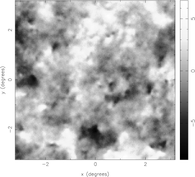
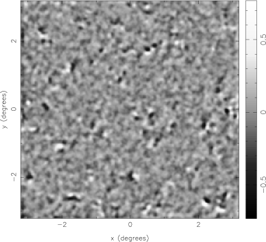
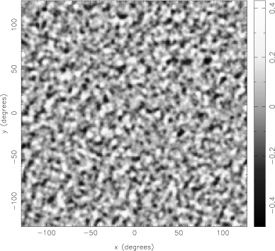
Figure 10: One of our non-Gaussian simulated maps with $b=1$ (top left) and an equivalent Gaussian realisation (top right). The bottom panels show the corresponding wavelet coefficients at scale $j=6$ for the à trous algorithm.

In spite of having only six different scales, that contain repeated information (since each region is comprised of the same number of wavelet coefficients as the original image) the separation of the models is better than that obtained with the tensor wavelets and comparable to the Mallat algorithm case (see Table 2).

In HJL, the case where Gaussian white noise is the main contaminant to the CMB map was also considered. This has been traditionally the greatest obstacle to the detection of non-Gaussianity in the CMB, and this is still the case for the 4-yr COBE data. However, current and future experiments are expected to produce data with a much higher signal to noise ratio and therefore this case offers less interest. Due to this fact and for the sake of brevity, we do no include this case in the present work. Nonetheless, we have repeated our analysis for maps where the rms level of instrumental noise is equal to that of the convolved CMB map and find that all the considered wavelets perform very well. In fact the two models are clearly discriminated being the power of the test $p=1$. We also find that the highest detection move towards larger scales. This is expected since the noise is most contributing at small scales, therefore obscuring the non-Gaussian signal.

5 Discussion and conclusions

We have investigated the performance of wavelet techniques to detect and characterise non-Gaussianity in the CMB, extending the work of Hobson, Jones & Lasenby (1999). Our test map consists of a realisation of the Kaiser-Stebbins effect due to cosmic strings of size $6.4$ square degrees and pixel of 1.5 arcminutes. In addition, a Gaussian component with the same power spectrum as the original signal has been superposed with Gaussian:non-Gaussian proportions $1:b$ and the resulting signal convolved with a Gaussian beam of $FWHM=5$ arcminutes. Gaussian white noise was also added with an rms equal to one-tenth that of the smoothed signal. A large number of non-Gaussian maps (10000) were generated, containing the same underlying Kaiser-Stebbins map and different realisations of the Gaussian component and noise. This allows us to account for the dispersion due to the Gaussian component and noise although the results will depend on the particular non-Gaussian underlying cosmic string map that is being used. Ideally, different non-Gaussian components should have been used for each map but generating cosmic strings maps is very computationally expensive and a large number of them were not available to us. However, these maps are still a good test for the method presented and, even if the particular level of discrimination may vary from realisation to realisation, we expect the general conclusions of this work to remain valid. The same number of Gaussian simulations were generated, simply by randomising the phases of the non-Gaussian maps. This method ensures that Gaussian and non-Gaussian realisations share the same power spectrum and thus any difference found between both models will be due to the non-Gaussian character of the signal and not to differences in the power spectrum.

The non-Gaussian test is as follows. First, we have obtained the wavelet transform of our non-Gaussian and Gaussian maps. We have then computed the fourth cumulant at each wavelet scale for each of the maps. All this information has been combined by computing the Fisher discriminant function for each simulated map and, finally, the distribution of this quantity has been compared for the Gaussian and non-Gaussian models. Indeed, the choice of a good test statistic that combines all the information from the different wavelet scales is crucial. The Fisher discriminant function is the optimal linear function of the measured variables in the sense of maximum power. In fact, we have found that, for most of our cases, the Fisher discriminant function clearly outperforms a generalised $\chi^{2}$ test.

We have also compared the performance of different wavelet transforms. Wavelets constructed using the Mallat algorithm have been shown to perform better than the 2D-tensor wavelets (used in the original work of HJL). In particular, using the Mallat algorithm, the stringy and inflationary models can be discriminated at a very high confidence level even when the Gaussian confusion has a rms twice as large as the one of the cosmic strings map ($b=2$, $p=0.995$ for Haar). However, the discriminating power of the test is clearly lower for the same case when tensor wavelets are used ($p=0.619$). In addition, we have tried different orthogonal bases for both decomposition schemes and find very similar results, providing all the information is combined into the Fisher discriminant function. In general, we have found that simpler wavelet bases perform slightly better than more complex ones. Thus we have used the Daubechies 4 and Haar wavelets for our work.

We have also investigated the performance of the à trous algorithm, a non-orthogonal wavelet transform. In spite of being redundant (each scale contains as many coefficients as the original image), its discriminating power is very similar to that of the Mallat algorithm. In particular, we find $p=0.991$ for $b=2$.

We have also addressed the problem of orthogonal wavelet transforms being sensitive to the orientation of the data, which is a consequence of the assymetry of the wavelet basis functions. To avoid this problem, we have used the Haar wavelet functions, which are antisymmetric. This means that the non-Gaussianity test is invariant under rotations of the data when the Haar wavelet is used. Another possibility is using a symmetric non-orthogonal wavelet such as the à trous algorithm. We have also presented results for Daubechies 4 for two different orientations of the data to give an insight of the sensitivity of the test when the original map is rotated.

In addition, wavelet techniques are useful to characterise the angular scale at which the non-Gaussian signal occurs. We have found the maximum non-Gaussian signal at scales $\sim 6$ arcminutes for the different considered transforms. Finally, we note that our test is not making use of the localisation property of wavelets. However, we can clearly see in the wavelet coefficients map of Fig. 10 individual patterns of the Kaiser-Stebbins effect. This shows that further wavelet algorithms can be investigated in order not only to detect the non-Gaussian signature of cosmic strings globally but also to extract individual non-Gaussian structures from the map.

References

- [] Aghanim N., Forni O., Bouchet F.R., 2001, A&A, 365, 341
- [] Aghanim N., Forni O., 1999, A&A, 347, 409
- [] Barreiro R.B., 2000, New Ast. Rev., 44, 179
- [] Barreiro R.B., Hobson M.P., Lasenby A.N., Banday A.J., Górski K.M., Hinshaw G., 2000, MNRAS, 318, 475
- [] Barreiro R.B., Martínez-González E., Sanz J.L., 2001, MNRAS, in press
- [] Barreiro R.B., Sanz J.L., Martínez-González E., Silk J., 1998, MNRAS, 296, 693
- [] Brandt S., 1992, ‘Datenanalyse’, 3rd edition, BI-Wissenschaftsverlag, Mannheim
- [] Burrus C.S., Gopinath R.A., Guo H., 1998, ‘Introduction to Wavelets and Wavelet Transforms. A primer’, Prentince-Hall, Upper Saddle River, New Jersey
- [] Coles P., 1988, MNRAS, 234, 509
- [1] Coles P., Barrow J.D., 1987, MNRAS, 228, 407
- [] Cowan G., 1998, ‘Statistical Data Analysis’, Oxford University Press, Oxford
- [] Daubechies I., 1992, ‘Ten Lectures on Wavelets’, S.I.A.M., Philadelphia
- [] Diego J.M., Martínez-González E., Sanz J.L., Mollerach S., Martínez V.J., 1999, 306, 427
- [2] Ferreira P.G., Magueijo J., Górski K.M., 1998, ApJ, 503, L1
- [] Ferreira P.G., Magueijo J., Silk J., 1997, Phys. Rev. D, 56, 4592
- [] Fisher R.A., 1936, Ann.Eugen., 7, 179; reprinted in ‘Contributions to Mathematical Statistics’, 1950, Jonh Wiley, New York
- [] Forni O., Aghanim N., 1999, A&AS, 137, 553
- [3] Gott III J.R., Park C., Juszkiewicz R., Bies W.E., Bennett D.P., Bouchet F.R., Stebbins A., 1990, ApJ, 352, 1
- [4] Heavens A.F., 1998, MNRAS, 299, 805
- [] Heavens A.F., Sheth R.K., 1999, MNRAS, 310, 1062
- [] Hobson M.P., Jones A.W., Lasenby A.N., 1999, MNRAS, 309, 125 (HJL)
- [] Hobson M.P., Jones A.W., Lasenby A.N., Bouchet F.R., 1998, MNRAS, 300, 1
- [] Holschneider M., Tchamitchian P., 1990, ‘Les Ondelettes en 1989’, ed. P.G.Lemarié, Springer Verlag, 102
- [] Kaiser N., Stebbins A., 1984, Nat, 310, 391
- [] Kogut A., Banday A.J., Bennett C.L., Górski K., Hinshaw G., Smoot G.F., Wright E.L., 1996, ApJ, 464, L29
- [] Magueijo J., 2000, ApJ, 528, L57 (see also Magueijo J., 2000, ApJ, 532, L157)
- [] Mallat S.G., 1989, IEEE Trans. Acoust. Speech Sig. Proc., 37, 2091
- [5] Martínez-González E., Barreiro R.B., Diego J.M., Sanz J.L., Cayón L., Silk J., Mollerach S., Martínez V.J., 2000, ApL&C, 37, 335
- [] Mukherjee P., Hobson M.P., Lasenby A.N., 2000, MNRAS, 318, 1157
- [] Naselsky P., Novikov D., 1995, ApJ, 444, L1
- [6] Pompilio M.P., Bouchet F.R., Murante G., Provenzale A., 1995, ApJ, 449, 1
- [] Scaramella R., Vittorio N., 1991, ApJ, 375, 439
- [] Shensa M.J., 1992, Proc. IEEE Trans. Signal Process, 40, 2464
- [] Starck J.L., Murtagh F., 1994, A&A, 288, 342