Towards Better Age Estimates for Stellar Populations:
The $Y^{2}$ Isochrones for Solar Mixture

Abstract

We have constructed a new set of isochrones, called the $Y^{2}$ Isochrones, that represent an update of the Revised Yale Isochrones (RYI), using improved opacities and equations of state. Helium diffusion and convective core overshoot have also been taken into consideration. This first set of isochrones is for the scaled solar mixture. A subsequent paper will consider the effects of $\alpha$-element enhancement, believed to be relevant in many stellar systems. Two additionally significant features of these isochrones are that (1) the stellar models start their evolution from the pre-main sequence birthline instead of from the zero-age main sequence, and (2) the color transformation has been performed using both the latest table of Lejeune et al., and the older, but now modified, Green et al. table. The isochrones have performed well under the tests conducted thus far. The reduction in the age of the Galactic globular clusters caused by this update in stellar models alone is approximately 15% relative to RYI-based studies. When the suggested modification for the $\alpha$-element enhancement is made as well, the total age reduction becomes approximately 20%. When post-RGB evolutionary stages are included, we find that the ages of globular clusters derived from integrated colors are consistent with the isochrone fitting ages.

1 Introduction

Isochrones are defined as the locus of coeval (equal age) points on the evolutionary tracks of stars of different masses in the Hertzsprung-Russell Diagram (HRD). An older isochrone has a fainter and redder main-sequence turn-off (MSTO), because the brighter and bluer massive stars evolve and die earlier. For the past four decades, astronomers have used this basic fact in various ways to derive the ages of star clusters and galaxies.

The first systematic application of the isochrone method was made to NGC 188 MSTO by Demarque and Larson (1964), as noted by Sandage and Eggen (1969). The widespread adoption of the isochrone technique has been tremendously helpful in understanding the formation and evolution of the Milky Way and its components, and the chronological sequence of astrophysical processes therein (see VandenBerg, Bolte, & Stetson 1996; Sarajedini, Chaboyer, & Demarque 1997). Today, isochrones are the most powerful means of measuring the ages of star clusters, and thanks to numerous recent improvements in the input physics, we may now claim to know the age of the Milky Way better than ever before. This purely theoretical achievement helps setting one of the most important constraints on cosmology, because the age of the universe is a distinctive product of any cosmological model.

A second-generation isochrone technique extends beyond the MSTO up to the tip of the red giant branch (RGB), to match more stars in the HRD (Iben 1974; Demarque & McClure 1977). The use of the extended isochrone, now standard, confers at least two significant advantages over the use of only the MSTO. Firstly, isochrone fitting is no longer in principle sensitive to the uncertainty in distance measurement. This advantage, however, has not practically been much appreciated because the uncertainties in the stellar atmosphere models and in the convection approximations still make it difficult to reproduce accurately the colors of red giants. Secondly, it allows us to build realistic population models for clusters and galaxies from their initial mass functions. This technique, called “evolutionary population synthesis” (EPS), was pioneered by Tinsley (1980).

In spite of the attendant difficulties, attempts to reproduce the colors and spectra of clusters and galaxies through the EPS technique are increasingly successful, and especially so when empirical stellar spectral libraries are resorted to (eg. Larson and Tinsley 1978; Gunn, Stryker, & Tinsley 1981; Bruzual 1983; Pickles 1985). The usage of isochrones has increased steadily. Notably, the recent studies of Spinrad et al. (1997) and Yi et al. (2000) have demonstrated that precision-isochrones can be used to constrain the galaxy formation epoch directly by estimating the ages of high-redshift galaxies in their youth. Such studies have demonstrated that population synthesis studies with precision-isochrones may even differentiate between various cosmological models.

Isochrones need to be updated when significant improvements are made in input physics. The Yale group (eg. Green, Demarque, & King 1987) is one among several involved in such activity. Other notable recent updates include Schaller et al. (1992), Straniero, Chieffi, & Limongi (1997), Girardi et al. (2000), and VandenBerg et al. (2000). The Yale group’s prior published set of isochrones, the Revised Yale Isochrones (Green et al. (1987): hereafter RYI), are out-of-date. A number of specialized studies have been published over the years by the Yale group which have updated the physics of stellar models (Guenther et al. 1992, 1996; Chaboyer & Kim 1995; Guenther & Demarque 1997; Yi et al. 1997; Chaboyer et al. 1998; Heasley et al. 2000). We note especially the importance of substantial improvements in the opacities and equation of state (mostly originating from the OPAL group: Iglesias & Rogers (1996)). Because of the need for a comprehensive set of isochrones for research in stellar populations, we hereby present a grid of Yale isochrones using up-to-date input physics and parameters.

Our new isochrone set (“the $Y^{2}$ Isochrones”, after the Yonsei-Yale collaboration) covers a wide range in metallicity and age. A wide $Z$-coverage in particular is useful in constructing EPS models for complex populations, such as elliptical galaxies. The ages in the $Y^{2}$ Isochrones are computed starting from the pre-MS birthline rather than from the “zero-age” MS (ZAMS). This allows us to build realistic young isochrones that are mainly defined by pre-MS stellar models. In this respect, they should be useful in population studies of youthful systems, such as young open clusters.

In this paper (the $Y^{2}$ isochrones-solar mixture), all isochrones are based on a chemical composition that has been scaled to the solar mixture. The case of $\alpha$-element enhancement will be considered in a subsequent paper. This is because we believe that we do not as yet have a clear understanding of it as a function of mass and of metallicity, particularly in the high metallicity regime. If $\alpha$-element enhanced isochrones is desired, we recommend the use of a correction formula similar to the one suggested by Salaris et al. (1993) with this set of isochrones. This correction formula has proven reliable in low metallicity systems, such as the globular clusters (Chaboyer et al. 1992), when compared to models actually constructed with opacities for $\alpha$-element enhanced mixtures. Subsequent work will present $Y^{2}$ isochrones that include $\alpha$-element enhancement based on more up-to-date opacities. Users will then be able to construct isochrones for the desired values of the $\alpha$-element enhancement via simple interpolation. The corresponding post-RGB models will also be available presently.

2 Input Physics and Parameters

The physics used in this study for the construction of stellar models is summarized in Table 1 and discussed below.

2.1 Microscopic Physics

The OPAL opacities are the most widely used Rosseland mean opacities today. Lately, the group has released newer tables for the Grevesse and Noels (1993) solar mixture that include the effects of seven additional heavy elements. These new calculations also include the effect of some changes in physics (Rogers & Iglesias (1995); Iglesias & Rogers (1996)). All these effects have been taken into account. We use the OPAL opacities for the temperature range of $\log T\geq 4.1$. For $\log T\leq 3.75$, we use the Alexander & Ferguson opacities (1994). In the temperature region of $3.75<\log T<4.1$, we use a value linearly interpolated between these two sets of tables. The conductive opacity is always included when $\log T\geq 4.2$ and $\log\rho\geq 2\times\log T-13$, where $\rho$ is density. We adopt the work of Hubbard & Lampe (1969) for $\log\rho\leq 6.0$ and the work of Canuto (1970) in the relativistic regime where $\log\rho>6.0$. Deep inside the star where the OPAL opacity table fails to cover, the electron scattering is the dominant mechanism.

The equation of state was taken from Rogers, Swenson, & Iglesias (1996), i.e., OPAL EOS. Beyond the boundaries of the table, the standard Yale implementation with the Debye-Hückel correction was used (Guenther et al. (1992); Chaboyer & Kim (1995)). The most popular equations of state have been simple Saha solvers, which we used when $\log T\leq 3.7$. As the importance of the Coulomb interaction has been acknowledged, the effect has been included using the Debye-Hückel approximation. Care has to be taken, however, that the Debye-Hückel correction is only applied when $\Lambda<0.2$ (see page 23-26 for definition of $\Lambda$ and discussion in Rogers (1994)). For masses of 0.75$M_{\odot}$ and above, $\Lambda$ is always less than 0.2 in the post-ZAMS stellar evolution models. Thus, models constructed using the OPAL equations of state and those of the usual Saha solver together with the Debye-Hückel approximation are similar (Chaboyer & Kim (1995)). Note that the treatment of Coulomb interaction in the OPAL equations of state are valid for values of $\Lambda$ up to 3, more than an order of magnitude better than the simple Debye-Hückel formula in common use. At very high temperature and/or pressure, where the OPAL EOS tables do not cover, we fall back to the YREC built-in EOS, which follows Cox & Giuli (1968), and is described in detail in Appendix A of Prather (1976). Here the pressure ionization is the dominant effect, i.e. fully ionized medium. Between tables, we have interpolated linearly.

To include helium diffusion in the calculation, we have employed Loeb’s formula (Bahcall, & Loeb 1990; Thoul, Bahcall, & Loeb 1994). For a more detailed discussion of diffusion, see Chaboyer et al. (1992) where the work of Thoul et al. (1994) and Michaud and Proffitt (1993) have been compared. There is an uncertainty in the diffusive coefficient of each metal element. Thus, common practice assumes that all heavy elements diffuse with the same velocity as fully ionized iron. Guenther & Demarque (1997) present the results of such computations. This study includes only helium diffusion.

The energy generation routines of Bahcall & Pinsonneault (1992) and the cross sections listed in Bahcall (1989) have been used. In addition, the cross sections for the $pp$ reactions, the $Be^{7}$-proton capture reaction, and the $hep$ reaction have been updated (Bahcall and Pinsonneault, priv. comm.). These routines, kindly provided by Bahcall (priv. comm.), also include coefficients for weak, intermediate and strong electron screening, based on the Salpeter (1954) theory of weak screening (which is valid in most cases in stellar evolution calculations), and its extension to intermediate and strong screening (DeWitt et al. 1973; Graboske et al. 1973). Neutrino losses from photo, pair and plasma neutrinos are included in the energy generation following the work of Itoh et al. (1989).

2.2 Solar Calibration

Our stellar models have been calibrated against the sun. These models are based on the solar mixture of Grevesse & Noels (1993). Grevesse & Noels made a major effort to determine more accurate CNO & Fe abundances, and now the solar Fe abundance agrees with the meteoritic abundance better than ever before. Their new solar metal-to-hydrogen ratio is $(Z/X)_{\odot}=0.0245$, while the previous value from Anders & Grevesse (1989), based on the meteoritic Fe, was 0.0267. The value we have finally adopted is 0.244 from the even more up-to-date value from Grevesse, Noels, & Sauval (1996).

The model that best matches the solar properties ($L_{\odot}$ = 3.8515E33 ergs $\rm s^{-1}$ and $R_{\odot}$ = 6.9551E10 cm) at the generally accepted age of the sun (4.50 Gyr) is of $(X,Z)_{0}=(0.7149,0.0181)$, i.e., $(Z/X)_{\odot}=0.0243$. Our solar model achieves the following agreements: $T_{\rm eff}/T_{\rm eff\odot}=0.999936$, log ($L/L_{\odot})=0.0000000185$, and log ($R/R_{\odot})=-0.0000006701$. At the solar age, the surface composition was (X, Z) = (0.7463, 0.0181). The mixing length parameter of $l/H_{p}=1.7432$ has been used to produce this match and thus for all other models.

Note that we have used the slightly larger value of $L_{\odot}$ (3.8515E33 ergs $\rm s^{-1}$) rather than the one listed in Livingston (2000), i.e., 3.845E33 ergs $\rm s^{-1}$. This 0.17% difference in luminosity is due to the uncertainty in the measured value of the solar irradiance. Guenther & Demarque (1992) state that “the luminosity has been determined from solar constant measurements from space on both the Nimbus 7 and the SMM satellites (Hickey & Alton 1983). ERB-Nimbus measures $\rm 1371.6\pm 0.765Wm^{2}$ and SMM/ACRIM measures $\rm 1367.7\pm 0.802Wm^{2}$ which yields luminosities of 3.846E33 erg $\rm s^{-1}$ and 3.857E33  erg $\rm s^{-1}$, respectively. As we cannot expertly base a preference, we merely take the average of the two and adopt the solar luminosity in all our models to be $L_{\odot}$ = 3.8515E33 erg $\rm s^{-1}$.” The accuracy of the Nimbus 7 measurements has more recently been estimated to be 0.5% (Lee et al. 1995). We simply adopt the value of $L_{\odot}$ from Guenther & Demarque (1992) in this study.

2.3 Chemical Abundance and $\Delta$$Y$/$\Delta$$Z$

We have set the initial chemical composition to $(Y,Z)_{0}=(0.23,0.00)$. Our solar calibration (described above) suggests the initial solar chemical composition of $(Y,Z)_{\odot}$ = (0.267025, 0.018100). This indicates $\Delta$$Y$/$\Delta$$Z\approx 2.0$, i.e.,

$$Y=0.23+2\,Z.$$ (1)

This slope is the same as that from VandenBerg et al. (2000) and only slightly smaller than that (2.25) of Girardi et al. (2000). Given the inevitable differences in codes and input parameters, we regard this as a good agreement. Table 2 displays the chemical compositions selected for this study.

It should be noted that $\Delta$$Y$/$\Delta$$Z$ is not a precisely determined quantity. In this study, it has been determined based on two values: the initial composition and the solar composition. Various techniques have indicated differing values, but most estimates cluster between 2 and 5 (see Pagel & Portinari 1998 for review). Adoption of a slightly different value does not greatly modify the stellar evolution when $Z$ is low. However, it can lead to unrealistic stellar models when $Z$ is very large ($>2Z_{\odot}$), because helium abundance is the prime factor in setting the pace of stellar evolution. In this sense, our extremely metal-rich models based on a crude value of $\Delta$$Y$/$\Delta$$Z$ may not have the same accuracy as their metal-poor counterparts.

2.4 Correction for $\alpha$-Element Enhancement

The isochrones presented in this paper are intended for solar-type populations that do not show signs of $\alpha$ enhancement. For populations with strong signs of $\alpha$ enhancement, such as metal-poor globular clusters, we recommend the correction formula similar to the one provided by Salaris, Chieffi, & Straniero (1993):

$$Z=Z_{0}(0.638f_{\alpha}+0.362),$$ (2)

or, one more appropriate to the Grevesse & Noels (1993) mixture, which is:

$$Z=Z_{0}(0.694f_{\alpha}+0.306),$$ (3)

where $f_{\alpha}$ is the chosen $\alpha$ enhancement factor, $Z_{0}$ is the actual metallicity of the target, and $Z$ is the metallicity of the appropriate non-$\alpha$-enhanced isochrone. The modification of the original Salaris et al. formula is necessary because of the change in the mixture adopted. This effect is probably small, as indicated by Salaris et al. (1993). But we also emphasize that such corrections are likely to be invalid at the higher metallicities.

Upon availability of our second set of isochrones (with $\alpha$ enhancement included), we will validate this issue and users will be able to generate the appropriate isochrones for any reasonable $\alpha$ enhancement factor through a simple interpolation.

2.5 Convective Core Overshoot

Convective core overshoot (OS), the importance of which was first pointed out by Shaviv & Salpeter (1973), is the inertia-induced penetrative motion of convective cells, reaching beyond the convective core as defined by the classic Schwarzschild criterion. Stars develop convective cores if their masses are larger than approximately 1 – 2 $M_{\odot}$, typical for the MSTO stars in 1 – 5 Gyr-old populations, depending on their chemical composition. Since the advent of the OPAL opacities, various studies have suggested a modest amount of OS; that is, OS $\approx 0.2$ $H_{p}$ for clusters of age 1 – 2 Gyr but OS $\approx 0.0$ – 0.1 $H_{p}$ for older clusters (4 – 6 Gyr), where $H_{p}$ is the pressure scale height (Stothers (1991); Demarque, Sarajedini, & Guo 1994; Dinescu et al. (1995); Kozhurina-Platais et al. (1997)).

In this study, we have adopted OS = 0.2 for younger isochrones ($\leq 2$ Gyr) and OS = 0.0 for older ones ($\geq 3$ Gyr). This is based on the observational studies listed above. It should be noted, however, that such tests of the models were performed mainly against the approximately solar abundance populations, and thus our adoption of the OS parameter may not be valid in chemically different populations.

For young isochrones with OS, we first found the critical mass $M^{conv}_{crit}$ above which stars continue to have a substantial convective core even after the pre-MS phase is ended, by inspecting the stellar models with no OS. The mass interval between our adjacent models being 0.1 $M_{\odot}$, the actual $M^{conv}_{crit}$ is between ($M^{conv}_{crit}$ listed) and ($M^{conv}_{crit}-0.1$). Then, we constructed heavier stellar models with OS included and used them in the construction of young isochrones. For old isochrones, we used stellar models with no OS regardless of mass. OS has many effects on stellar evolution (see Stothers 1991). Among the most notable are its effects on the shape of the MSTO, on the rate of evolution near the MSTO and the subgiant phase, and on the ratio of total lifetimes spent in the core hydrogen burning stage (MS) and in the shell hydrogen burning stage (RGB). The impacts of such effects on the isochrone and on the integrated spectrum have been discussed by Yi et al. (2000).

3 Construction of Stellar Models

3.1 Evolutionary Tracks

We have used the Yale Stellar Evolution Code (YREC) to construct these stellar models. In order to construct the isochrones for the age range 0.1 – 20 Gyr that extend to the tip of the RGB, we have constructed evolutionary tracks for mass 0.4 – 5.2 $M_{\odot}$, from the pre-MS birthline to the onset of helium burning. In addition to these full isochrones, we also provide younger isochrones that reach only up to the upper MS, as explained in §5.

3.2 Initial Models at Pre-MS Birthline

An important improvement of the $Y^{2}$ isochrones over RYI is the fact that these stellar models begin, not at the classic ZAMS, but at the deuterium MS, also called the “stellar birthline”, where stars initially become visible objects (Palla and Stahler 1993), during the pre-MS stage. Thus, these models include pre-MS evolution.

The pre-MS lifetime, denoting the time taken by a star to evolve from the birthline to the ZAMS, is a strong function of stellar mass, varying from less than 1 Myr to about 200 Myr for stars in our mass range. It is about 43 Myr long for a solar mass model. This means that the ZAMS, as hitherto defined, has an inherent age spread of about 200 Myr, making it simply inappropriate to use models starting from the ZAMS to match the HRDs of young clusters. Because of this, isochrones that label ZAMS stars as “zero-age” are bound to mismatch the lower part of the observed HRDs of young clusters that contain pre-MS stars (e.g. Patten & Pavlovsky 1999). This effect is negligible in old ($>1$ Gyr) populations, causing age underestimates of only 1% for 10 Gyr populations, but it can be significant in the analysis of young open clusters. We therefore suggest that ages be henceforth defined relative to the birthline rather than the ZAMS.

In view of the expanding utility of isochrones beyond the treatment of old systems, in recognition of the increasing importance of very young systems, and to provide a unified treatment for open, globular and perhaps other star systems, we have decided to include pre-MS evolution in this set of isochrones.

This raises the issue of where and how the models should be started off. Is there some equivalent of the ZAMS on the Hayashi track? One cannot begin the evolution at an arbitrary point on the pre-MS, since the radius and the central density of stars, both important quantities, especially from the viewpoint of stellar rotation, but also in a more general sense, change rapidly during this phase. This deprives us of the pause on the MS, when hydrogen burning begins, that serves as a natural starting point for models relevant to old stellar populations. An equivalent of this pause is provided by the deuterium MS, or stellar birthline, as defined by Palla and Stahler (1991). Its use for these purposes seems both apposite and physically meaningful. For the low-mass stars in this study, the birthline is distinct from and above the MS, located just above the T Tauri stars in the HRD.

We have constructed a series of birthline models for low-mass stars on the birthline. These models are then evolved forward in time along the pre-ms tracks, onto the MS and beyond, ending at the RGB tip, but thus making available isochrones intended for quite young systems as well, perhaps valid even for 10 Myr-old systems.

Operationally, these models were started off from polytropic models that were placed even higher than the birthline in the HRD. However, polytropic models are quite different from real stellar models in their thermal structure. Thus they need to be relaxed until their thermal structures are correct. This is accomplished in YREC and the resulting structures are evolved down their Hayashi tracks until they satisfy the mass-radius relationship of Palla & Stahler (1991), at which point they are assigned age zero (see also Barnes & Sofia [1996]). This pre-birthline evolutionary phase is a convenient way of calculating physically self consistent initial models, and has no special physical significance since it does not include deuterium burning in the definition of the birthline. Deuterium burning is however implicitly included in the post-birthline evolution in the reaction network of YREC. The initial deuterium gets destroyed, but the contribution of deuterium burning to the total energy production is negligible compared to the contribution from gravitational contraction. Thus, the starting models have both the correct, or at least appropriate, radius and also internal structure. The chemical composition is now checked, and adjusted to be pristine. Models with differing chemical compositions may be constructed by rescaling the corresponding solar mixture models. A series of these models have been constructed for different masses. These models are then evolved onto the MS and beyond.

4 Color Transformations

Theoretical properties ([Fe/H], $L$, $T_{\rm eff}$) have been transformed into colors and magnitudes using the color transformation tables of Lejeune, Cuisinier, & Buser (1998, hereafter LCB) and of Green et al. (1987, hereafter GDK), which was used in the RYI. Both tables are semi-empirical: the LCB table is based on the latest Kurucz spectral library (1992) and the GDK table is based on the older Kurucz library (1979). Both tables have been substantially modified to match the empirical stellar data better than their forebears (Kurucz tables) and extended to low temperatures based on empirical data and low temperature stellar models. For the present calculations, we have used the updated BaSeL-2.2 version of the LCB library, for which the calibration of the cool giant models in the parameter ranges 4500 K $\leq T_{\rm eff}\leq$ 6000 K and 2.5 $\leq{\rm log}\,g\leq$ 3.5 has been revised.

In the process of comparing isochrones to observation, the adoption of an up-to-date color transformation table is as important as updating input physics in the construction of stellar models. The difference between the LCB table and the GDK table is substantial, as shown in Figures 1 and 2. Figure 1 shows the comparison of bolometric correction ($BC$) for ${\rm log}\,g=4.5$ MS stars. The overall agreement is good. At solar metallicity and temperature (vertical line in the top right panel), $BC$ from the LCB table is somewhat higher than that from the GDK table. For example, $BC_{\odot}$ is $-0.08$ and $-0.109$ in the GDK table and in the LCB table, respectively. We have normalized these two tables to the Sun so that the visual absolute magnitude of the Sun ($M_{V\odot}$) becomes 4.82 (Livingston 2000), regardless of the table used. Then, the following definition of $BC$:

$$BC=M_{bol\odot}-M_{V}$$ (4)

yields $M_{bol\odot}=4.711$ and 4.74 for the LCB table and the GDK table, respectively. Because $M_{V}$ is defined as:

$$M_{V}=M_{bol\odot}-2.5{\rm log}L/L_{\odot}-BC,$$ (5)

the two tables yield the same $V$ magnitudes.

Figure 2 shows how seriously the two color tables differ from each other. The original GDK table reaches only down to the effective temperature of 2800K and up to 20000K. In order to cover the tip of the metal-rich RGB ($Z\geq 0.06$), we have extrapolated this table down to 2500K when necessary. A few of the youngest and most metal-poor isochrones reach above effective temperature 20000K. In that case, we have used the colors from the LCB table. This crude remedy did not cause any noticeable discontinuity in the isochrones.

The LCB table is obviously more up-to-date than the GDK table. Yet, it is not always our preference. In some circumstances, the isochrones with the GDK table match the empirical data better. However, without knowing the true parameters (metallicity, reddening, and distance modulus), it is difficult to choose one over the other. Thus, we have decided to provide our isochrones in two formats based on both tables. Users are recommended to try both. The color transformation is for the filter systems of $(UBV)_{Johnson}(RI)_{Cousins}$ in the GDK table and of $(UBV)_{Johnson}(RI)_{Cousins}(JHKLM)_{ESO}$ in the LCB table.

5 Results

5.1 Stellar Evolutionary Tracks

Figure 3 shows a sample set of stellar evolutionary tracks for the solar composition and for the mass range of 0.4 – 5.0 $M_{\odot}$. The line connecting the diamond symbols is the birthline for this composition. The first position of each track in the HRD is somewhat uncertain because it depends on the choice of the first time step in the numerical computation. This uncertainty can be alleviated if we force the first time step to be very small. However, we have decided not to pay too much attention to such details in the first steps of the pre-MS stage because we believe that other uncertainties in the position of the birthline and in observational data are much larger. In this sense, our youngest isochrones below 10 Myr are less certain than their older counterparts.

5.2 Isochrones

Figure 4 shows a set of isochrones for $Z=0.02$ and ages of 1 Myr through 20 Gyr. The young isochrones (1, 2, 4, 8, 10, 20, 40, 60, 80 Myr) are complete only to the MS and thus focused on the pre-MS stage. As mentioned earlier, one of the most notable features of the $Y^{2}$ Isochrones is the inclusion of pre-MS stellar evolution.

The information that we provide in the $Y^{2}$ Isochrones is listed in Table 3. The last three columns are luminosity functions (LFs); namely, the number of stars in the box defined by the mass grid given assuming there were initially 1000 stars in the mass range of 0.5 – 1.0 in $M_{\odot}$, following the concept introduced in the RYI. The bottom right panel in Figure 4 shows the evolution of LF in the case of IMF slope $x=1.35$ (Salpeter index).

Figure 5 compares the $Y^{2}$ Isochrones and RYI. One can see the substantial change in the stellar models in the top left panel. The other three panels show the isochrones in the observer’s HRD. The effects of the use of the LCB color transformation table are clear. With a close inspection of the lower MS of some isochrones based on the LCB table, one will find some discontinuities in $U-B$ and $B-V$ colors (e.g., lower left panel). These are partly real because they are also present in the empirical data, although with a smaller amplitude. The discontinuities in the isochrones get amplified by the fact that the empirical data are scarce especially in terms of metallicity and gravity grids. Besides, the adjustment (correction) between the Kurucz spectral library (the foundation of our color tables) and the existing low temperature libraries made by LCB is not as feasible as we had hoped for because of the large and apparent difference between them (At times, the flux difference is as large as an order of magnitude).

Similarly, peculiarly curved features on the RGB tip are shown in the LCB-based isochrones (in $U-B$ and $B-V$ colors). These features are caused by the non-monotonic temperature-color relations that are present in the empirical data. Lejeune et al. (1997, Figures 6 & 14) illustrate these effects. Whether the empirical stellar data that show such non-monotonic temperature-color relations are being correctly interpreted and implemented in the color transformation table remains to be determined through more rigorous data sampling. Because of the limitation of the adopted calibration procedure by LCB, the corrected LCB colors still differ from the empirical data by as much as 0.1 mag in $U-B$ and $B-V$ (see for instance Figure 14 in LCB). In this sense, our LCB-based isochrones are subject to such uncertainties. Readers are referred to Lejeune et al. (1997; 1998) for more information. Despite the magnitude of the disagreement in the colors in this temperature range (often up to 1 mag!), this may not be an important issue in the study of most Milky Way globular clusters, because their metallicities are too low to be affected by this uncertainty. But it is a serious problem in metal-rich stellar populations of the kind found in the bulges of spiral and elliptical galaxies.

Part of a sample isochrone is shown in Table 4. The tables in their entire form are available electronically from this paper. Minor corrections may occur to the tables after publication. The updated versions will be available from the authors upon request or directly from our WEB site. We also provide a FORTRAN interpolation routine that works for metallicity and age interpolation via the same WEB site.

5.3 Bump on the Red Giant Branch

The evolution in luminosity on the RGB is not always a monotonic function of time. When the depth of the convective envelope increases, some processed material is distributed over the entire convective region, and CNO processed isotopes are mixed to the surface. Stars are rejuvenated by such mixing because unprocessed hydrogen is mixed from the envelope into the interior. The first, and largest, of these partial mixing phenomena on the RGB, is called “first dredge up”, an event which takes place when the star’s convection zone reaches its maximum depth soon after it reaches the giant branch. The convection zone depth then decreases (in terms of mass fraction) as the star evolves up the giant branch, leaving behind a composition discontinuity. At some later point, the hydrogen burning shell passes through the composition discontinuity. This event gives rise to a temporary decrease in luminosity, as shown in Figure 6. This was predicted by Thomas (1967). This results in a peak in the luminosity function on the RGB, or “bump”, which is observed in some globular clusters (see e.g. King et al. 1985; Fusi Pecci et al. 1990). At luminosities higher than the bump on the giant branch, stars will have more fuel to burn in the upper part of the RGB, because the first dredge-up had previously mixed in fresh hydrogen from the envelope.

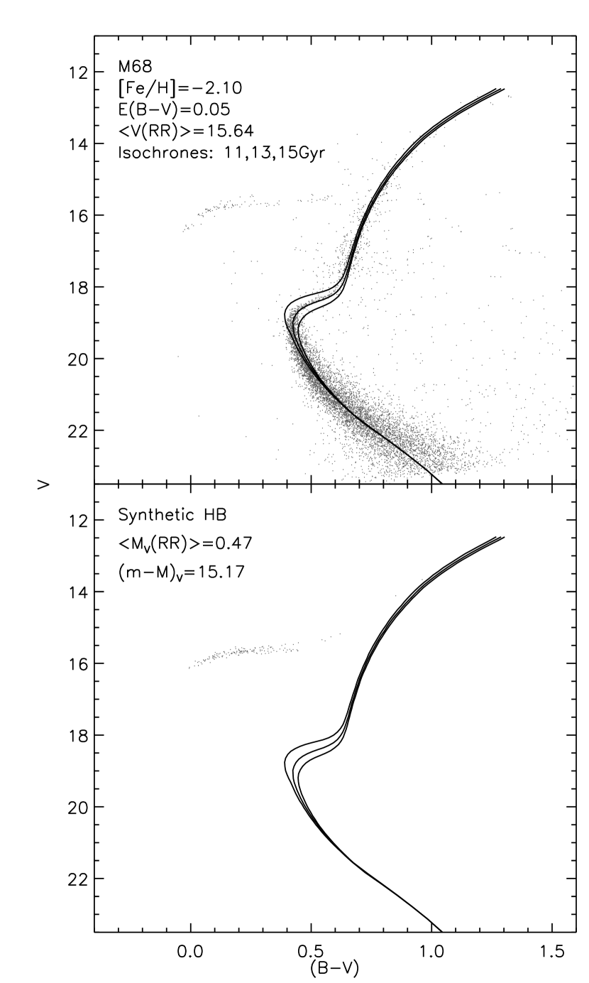
Figure 13: Same as Figure 12 but for M 68. The HRD data are from Walker (1994). The estimates of [Fe/H] and reddening are from Harris (1996), and [$\alpha$/Fe]=0.3 has been adopted following the halo observations.

Figure 7 and Table 5 display the predicted position of the RGB bump as a function of age and metallicity. Except when the metallicity is extremely low, the RGB bump generally gets fainter as age and metallicity increase. We have also plotted in Figure 7-(b) the $V$ magnitudes of the RGB-bumps in some globular clusters. The $V$ brightness data are from Table 4 in Fusi Pecci et al., while the distance moduli and the metallicities are from Harris (1996). In the case of 47 Tuc (the second most metal-rich data point), we have adopted a distance modulus of 13.47 from our CMD fit described in Figure 13. The most metal-rich data point ($V(bump)\approx 17.1$) has been derived from the NGC 6553 data from Zoccali et al. (2001). Adopting [Fe/H]=$-$0.17 (see §7.3), we derived $M_{V}(bump)\approx 1.3$, which is also in good agreement with the prediction.

The prediction of the position of the RGB bump cannot be precise because of the uncertainties in the detailed physics at the base of the convection zone and the dynamics of the first dredge-up. When the RGB bump was first identified in 47 Tuc (King et al. 1985) the observed RGB bump luminosity then differed from the predicted luminosity in the theoretical tracks, and possible causes for this discrepancy were explored, principally convective overshoot below the convection zone, and opacity uncertainties. Subsequent improvements in the quality of the observational data and in the opacities and other physics input have resulted in a decrease in the discrepancy (Fusi Pecci et al. 1990). More recently, some researchers have argued that the discrepancy disappears when one takes into account the opacity increase due to alpha-enhancement and that the effect of convective overshoot is negligible (Cassisi and Salaris 1997; Ferraro et al. 1999).

We note at this point that other physical processes can play an equally significant role. The presence of mixing other than convective overshoot complicates the issue. There is evidence that some mixing below the convection zone takes place in red giants, probably the result of meridional circulation due to rotation (Sweigart & Mengel 1979). Near the MS, the envelope overshoot does not seem sufficient to explain the observed lithium depletion below the convective envelope (Pinsonneault 1994). We also note that helioseismological inversions indicate that there is little overshoot below the convection zone in the present sun (Basu, Antia, & Narasimha 1994). For all these reasons, our models were calculated without any overshoot below the convection envelope. The effects of including alpha-element enhancement on the RGB bump position will be discussed in our next paper.

5.4 Maximum Brightness of the RGB

In general, the RYI did not provide accurate positions of RGB tips, because until recently isochrones were dominantly used for HRD fitting, a matter in which the RGB tip plays a small, if any, role. However, isochrones are now used in a variety of studies. One example is a field of evolutionary population synthesis, whose aims include the computation of integrated properties (eg. colors and magnitudes) of stellar populations. The position of the RGB tip is important in computing near infrared magnitudes, as stars near the RGB tip are good infrared sources. Therefore, we have paid extra attention in order to define the RGB tip as consistently as possible. It should be noted, however, that evolution near the RGB tip remains somewhat uncertain, and will remain so as long as mass loss is poorly understood.

Another important application of accurately modeled RGBs is to use them as distance indicators for metal-rich populations. Figure 8 shows that the brightness in $V$ magnitude on the RGB reaches a maximum not at the RGB tip but in the middle of the RGB. Because the number density of stars in the middle of the RGB is much higher than that of the RGB tip, this gives us a large statistical advantage. Besides, this part is more certain than near the RGB tip in terms of our understanding of stellar evolution. This effect, however, occurs only when the metallicity is high enough, i.e., $Z\gtrsim 0.004$, because it is mainly an opacity effect. There are currently a great number of observational studies that are based on this concept. New predictions are provided in Figure 8 and Table 6.

6 Luminosity Functions and Photometric Evolution

Isochrones are convenient building blocks for the the study of evolutionary population synthesis (EPS). EPS studies either use the luminosity functions (LFs) provided in the isochrone tables (if provided as is the case with our isochrones) or compute the LFs using the mass information that is always provided in the isochrones. Generating isochrones is not a trivial matter partly because keeping the desired accuracy in mass through several track interpolations is not easy. As Yi et al. (2000) mentioned, the mass difference between the bottom and the tip of the RGB in the 12 Gyr isochrones is merely an order of 0.7% or approximately 0.006 $M_{\odot}$. If the mass interpolation is inaccurate in the 5th decimal place in $M_{\odot}$, the LF will lose its desired accuracy. Such errors can be checked by inspecting the integrated photometric properties of a sample population, as shown in Figure 9. Our isochrones all show clear and smooth luminosity (and color) evolution, except where there are expected departures from the monotonicity in the color transformation table. Considering this complexity, it is better to use the isochrones rather than stellar tracks in most of the EPS studies.

7 Tests of Isochrones against Empirical Data

We are encouraged by the fact that the improved isochrones actually provide a better match to the empirical data. In this section, we display some of the tests we have made. We have attempted to provide a variety of tests to check the validity of different aspects of the isochrones. For example, we try to test our isochrones on young open clusters as well as old globular clusters. We demonstrate the level of agreement between the isochrones and the MS stars in the field as well as in an open cluster. We also present a test of the color evolution of Galactic globular clusters. We are pleased to find that our isochrones combined with their LFs reproduce their integrated colors quite well at their generally accepted ages.

7.1 Population I MS stars

One of the most basic tests is to examine whether our stellar models match the measured properties of nearby MS stars. Figure 10 shows a set of stellar evolutionary tracks for $Z=0.02$, i.e., nearly solar. Overplotted are the observed MS stars from Gray (1992). The match is good: not only do the models match the locus of the observed MS, but the match in mass is also good except in the very low mass range ($M\lesssim 0.6$ $M_{\odot}$). The masses of the faintest three data points (M dwarfs) are 0.6, 0.52, and 0.48 $M_{\odot}$ according to Gray (1992), while models suggest approximately 0.7, 0.6, 0.58 $M_{\odot}$. This disagreement in mass in the low mass range may be due to the uncertainties in the mass determination of cool stars or in the low-temperature stellar atmosphere models.

7.2 Subdwarf MS Stars

Figure 11 shows the match between our isochrones and the subdwarf MS stars whose distance has been determined through HIPPARCOS observations. The data are from Reid (1998), and we have followed the same criteria for the data selection as VandenBerg et al. (2000) did for their Figure 14: i.e., $[Fe/H]\,<\,-0.55$, $M_{V}\,>\,4.5$, and $\sigma_{\pi}/\pi\,<\,0.07$. Instead of 14 Gyr isochrones, we are using 12 Gyr isochrones. However, there is practically no difference in this part of the isochrones. Since our isochrones do not include the effects of $\alpha$-element enhancement, we have recalibrated to compute the isochrones in this plot using Equation [2]. We have adopted [$\alpha$/Fe]=+0.4 and +0.2 for [Fe/H]$\leq-$1.0 and [Fe/H]=$-$0.5, respectively, following Wheeler, Sneden, Truran (1989) and Carney (1996). The agreement is good and is marginally better with the isochrones based on the GDK table.

7.3 Globular clusters

Globular clusters are the main targets of isochrone applications. They are the playgrounds of stars of the same age and metallicity, so we can test and refine our stellar models. Moreover, an accurate estimation of their ages has been appreciated as an important route to a better understanding of cosmology.

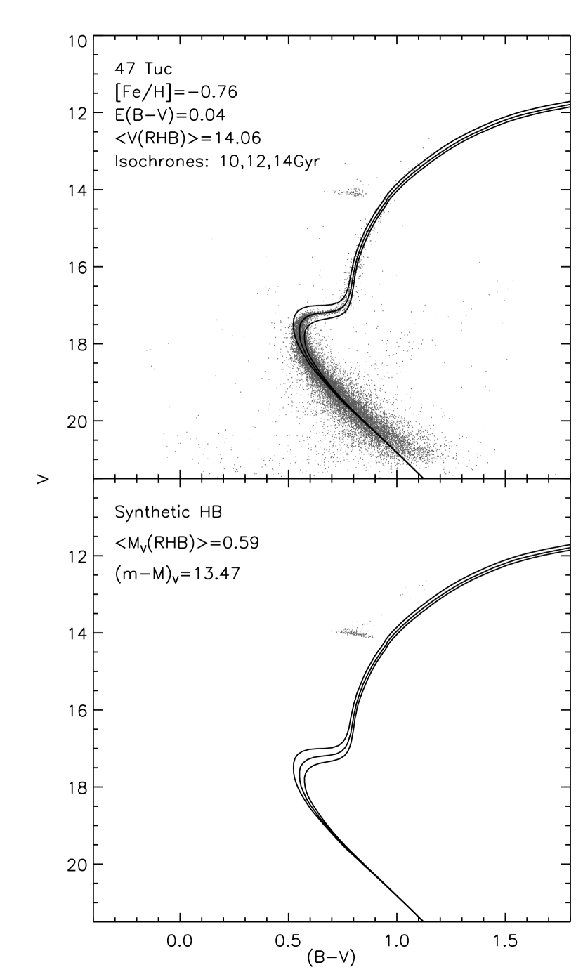
Figure 12: A test to the HRD of 47 Tuc. The HRD data have been kindly provided by A. Sarajedini. The estimates of [Fe/H] and reddening are from Harris (1996). [$\alpha$/Fe]=0.15 adopted following the general pattern in the halo.

Figures 12 and 13 shows fits to the metal-rich cluster 47 Tuc and the metal-poor cluster M 68, using our isochrones based on the GDK table. We have used theoretical values of $M_{V}$(RR) from Demarque et al. (2000) to derive their distances. These models are based on the HB evolutionary tracks with input physics nearly identical to the current isochrones. They also take into account the effects of HB morphology in the calculation of $M_{V}$(RR) for a given [Fe/H]. The theoretical values of $M_{V}$(RR) from these models are in a reasonable agreement with RR Lyrae luminosities derived from the main sequence fitting of globular clusters based on HIPPARCOS parallaxes for field subdwarfs (Reid (1997); Gratton et al. (1997)). For purposes of illustration, we have shown synthetic HB models in the lower panels (see Lee, Demarque, & Zinn 1994 for description).

In case of 47 Tuc, its red HB is approximately 0.15 mag brighter than RR Lyrae level. The matches are good if their ages are approximately 12 and 13 Gyr, respectively. Through the tests on a few other globular clusters, we have found a reduction in the age estimates of the order of 20%, and this is when $\alpha$-enhancement has been considered using the Salaris et al. formula.

The primary source of this age reduction is the update of the stellar models. Of several ways to measure the ages of globular clusters, the most popular one is probably to match the MSTO luminosity using isochrones. The $Y^{2}$ isochrones are fainter at the MSTO (bluest point on the MS) than the RYI by approximately 16% when $Z=0.0004$, a metallicity typical for Galactic globular clusters. Figure 14 clearly shows this. A given observed MSTO luminosity indicates substantially younger ages when the $Y^{2}$ isochrones are used. Also compared in this figure is the result derived from the isochrones of Girardi et al. (2000), whose input physics is quite compatible to ours. The agreement with our models is good.

Table 7 shows the change of the derived ages caused by the use of the new stellar models alone. The estimates are the mean values of the age estimates for various values of MSTO luminosities within the range of 5 – 16 Gyrs. Much of this age reduction is caused by the inclusion of the the helium-diffusion and the use of the updated equations of states. Our preliminary investigation suggests that, in addition to this, the inclusion of alpha-enhancement causes approximately another 5% of age reduction. It should also be noted that the change (reduction) in derived ages caused by the improvement in the stellar models alone (no alpha-enhancement effects included) is reversed in the metal-rich regime (see Table 7). These issues will be discussed more thoroughly in our next paper.

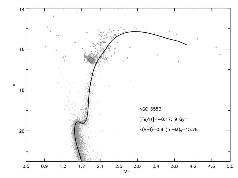
Figure 15: A test to the HRD of the metal-rich cluster NGC 6553. The new isochrone (based on the LCB color table) matches the overall HRD well at 9 Gyr. The data are from Zoccali et al. (2001; small dots) and from Sagar et al. (1999; crosses). The open diamond is from our synthetic HB models.

The next test is on NGC 6553, a metal-rich Galactic globular cluster (Figure 15). The faint data (dots) are from Zoccali et al. (2001). They are confirmed members of the cluster. Also shown are the bright stars ($V<17$: crosses) from Sagar et al. (1999). They have been selected to satisfy $Error(V-I)<0.2$. These two data sets have offsets both in $V$ magnitude and in $V$-$I$ by 0.3 mag and 0.15 mag (the Zoccali et al. data being brighter and bluer), respectively. This is because the Zoccali et al. data are from the region that suffers less reddening (Zoccali, priv. comm.). When we shifted the Sagar et al. data, both sets match one another from the MS to the HB clump very well. The magnitudes of the offsets were estimated from the mean positions of the HB clump through eye-fit.

The metallicity of this cluster has been reported to be in the range of [Fe/H]=$-$0.5 – +0.1 (see Sagar et al. 1999), i.e. approximately $Z\approx$ 0.006 – 0.02. We have adopted $Z$=0.0125 ([Fe/H]=$-$0.17) in this study because at this metallicity the LCB-based $Y^{2}$ isochrones match the upper RGB of this cluster best. The age of the model (9 Gyr for this fit, $E$($V$-$I$)=0.9, $m$-$M$[apparent]=15.78) has been derived from the luminosity difference between the MSTO and the mean luminosity of the HB clump. The open diamond shown on top of the HB clump is the synthetic HB clump for this age and metallicity. However, the age estimate is sensitive to the adopted metallicity; 10 – 8 Gyr when $Z$=0.01 – 0.02. Zoccali et al. (2001) achieve a somewhat larger age estimate, 12 Gyr, but this is mainly because they assume a metallicity lower than ours. Using LCB-based $Y^{2}$ isochrones, we favor our metallicity and thus a smaller age.

The match by the LCB-based $Y^{2}$ Isochrones is good. The turn-around in the $V$ magnitude would not be as dramatic as observed if the GDK table is used, although GDK-based isochrones seem to match the MS better. Considering the importance of this bulge cluster to the study of the formation of Milky Way, a more careful analysis, in particular considering $\alpha$-enhancement (highly suspected to be present [B. Barbuy, priv. comm.], is required to give a definite answer.

7.4 Open clusters

If tests against globular clusters teach us about the stellar evolution in the MS and phases beyond, those against young open clusters teach us about pre-MS stellar evolution. Several studies have noted that the theoretical isochrones are fainter in the lower MS than observed (e.g., Subramaniam & Sagar 1999; Patten & Pavlovsky 1999). This is likely to be evidence of pre-MS evolution.

Figures 16 and 17 show isochrone fits to the young open clusters, Pleiades and IC 2391. Both LCB- and GDK-based isochrones work well for these fittings. The Pleiades data are very well represented by the 40–100 Myr isochrones, assuming $E(B-V)=0.04$ and $m-M$(apparent)=5.6 (Pinsonneault et al. 1998). A good fit requires an apparent distance modulus somewhat larger than that derived from the HIPPARCOS data, as was noted earlier by Pinsonneault et al. (1998).

The overall fit appears to be good, but the data at $B-V\approx 0.5$ and $\gtrsim 1.5$ seem to be notably brighter (or redder) than the models. If the observational errors are not to be considered large, this may indicate the shortcomings of the models.

The MS data of the younger cluster IC 2391 is matched by the 20 Myr solar-composition isochrone. This is reasonably close, if somewhat smaller than the age estimate of Patten & Pavlovsky (1999), i.e. 30 Myr. The membership study of this cluster has been performed very carefully, and thus the data are of good quality and the sequence is better defined than the data shown in Figure 16. The model isochrones are for 4, 10, 20, 40, and 80 Myr of age, while the 20 Myr isochrone is marked as thick line. The 20 Myr isochrone appears to be matching the data reasonably well, but this pre-MS isochrone does not fully reproduce the curvatures at $V-I\approx 2$. A similar but larger mismatch was reported by Patten & Pavlovsky (1999; see their Figure 3). It seems that the $Y^{2}$ Isochrones match the data better in the lower MS (cross symbols in Figure 16) than the fit shown in their Figure 3, which was based on a different set of isochrones.

The level of agreement between the model and the data may not yet be satisfying to some readers. However, we are quite impressed by the matches, considering the large uncertainties still embedded in the convection approximation in cool stars and their color transformation. Fits to open clusters involve complex considerations of membership, photometry of differing quality for stars in differing magnitude ranges, (differential) reddening, metallicity, and of course, distance, all of which impinge on the age assigned. Inconsistencies are often found and resolved only in the context of detailed studies, and we invite the community to use these isochrones in such contexts.

7.5 Photometric Evolution

One of the most exciting outcomes of our isochrone tests is that the integrated colors can be practically used as reliable age indicators of simple stellar populations. Astronomers have long been aware of this fact, but the level of the accuracy of integrated colors as age indicators has never been very high. Optical integrated colors were believed to be useful in determining whether a population is 5 Gyr or 15 Gyr, but not whether it is 10 Gyr or 13 Gyr; that it, the expected accuracy was of an order of 50%. This is because the color evolution of old populations is too slow to be useful as an age indicator. In this paper, we claim that we have achieved a substantially better precision. Figure 18 shows the mean integrated colors of Galactic globular clusters (Harris 1996) compared with the models. Thin lines are the models made of only MS and RGB stars and thick lines are the complete models with all phases including HB stars. When complete models are used, the mean colors of the Milky Way clusters indicate ages of 12 – 13 Gyr, which is virtually identical to the age estimates obtained from the isochrone fitting. If this is not a coincidence, this improvement in the predictability of integrated colors as a function of age and metallicity will be useful to many applications in the population study.

8 Conclusions

If the HRD opened the window into the details of stellar evolution, it is isochrones that made the knowledge of stellar evolution practically meaningful to other areas of astronomy.

In this first paper, we publish a set of isochrones in which the heavy elements are scaled to the solar mixture. The use of the solar mixture is quite appropriate for the study of many stellar populations with approximately solar relative abundances. Isochrones to the tip of the giant branch for ages ranging from 0.1 to 20 Gyr have been constructed for metallicities $Z$ between 0.00001 and 0.08. Additional isochrones with ages down to 1 Myr are also provided for the pre-MS and the MS phases only.

A follow-up paper will consider mixtures that are enhanced in $\alpha$-elements as compared to the sun, since many pieces of evidence suggest $\alpha$-element enhancement in metal-poor stars and some metal-rich populations. Meanwhile, the reader is provided with a convenient correction formula for $\alpha$-element enhancement. This formula has proved reliable in the case of metal-poor stars in the field and in globular clusters which are believed to be $\alpha$-element enhanced.

Important advantages of the $Y^{2}$ Isochrones over the RYI are as follows. (1) The $Y^{2}$ Isochrones are based on updated input physics. (2) They are available for the more up-to-date color transformation table of Lejeune et al. (1998), as well as for the Green et al. table used for the RYI. (3) The stellar models start their evolution from the pre-MS birthline instead of from ZAMS. This makes the $Y^{2}$ Isochrones the first comprehensive isochrones (covering a large range of age and metallicity) based on the stellar models that include the pre-MS stage. This fact makes the $Y^{2}$ Isochrones useful to young open cluster studies as well. (4) Convective core overshoot has been taken into account. This has important impacts on isochrone fitting to open cluster HRDs and to the spectral dating of intermediate-age populations.

We note that the $Y^{2}$ Isochrones match the properties of observed objects much better than the RYI. In particular, good matches are achieved at substantially smaller ages than before for the Galactic globular clusters, by approximately 20%, once $\alpha$-element enhancement corrections are taken into account. Approximately 15% (out of 20%) of this age reduction is caused by the update in the stellar models.

Partly owing to the improved color calibration, and partly due to the inclusion of post-RGB evolutionary phases, the model integrated colors generated by the isochrones now also match within the uncertainties the observed integrated colors of Galactic globular clusters at their expected ages. This is one of the most significant achievements made by the $Y^{2}$ Isochrones.

The $Y^{2}$ isochrones are available from the authors upon request or directly from our WEB site, as well as electronically through this paper. We are currently constructing a new set of $\alpha$-element enhanced $Y^{2}$ Isochrones.

Table 1: Input Physics and Parameters

Solar mixture	Grevesse & Noels (1993)
OPAL Rosseland mean opacities	Rogers & Iglesias (1995), Iglesais & Rogers (1996)
Low temperature opacities	Alexander & Ferguson (1994)
Equations of state	OPAL EOS (Rogers et al. 1996)
Energy generation rates	Bahcall & Pinsonneault (1992; 1994 priv. comm.)
Neutrino losses	Itoh et al. (1989)
Convective core overshoot	0.2 $H_{p}$ for age $\leq$ 2 Gyr
Alpha-element enhancement	none
Helium diffusion	Thoul et al. (1994)
Mixing length parameter	${\it l}/H_{p}=1.7431$
Primordial helium abundance	$Y=0.23$
Galactic helium enrichment parameter	$\Delta$$Y$/$\Delta$$Z=2.0$

Table 2: Chemical Compositions and Convective Core Developing Mass

$Z$	$Y$	[Fe/H]	$M^{conv}_{crit}$
0.00001	0.23002	-3.29	2.1
0.00010	0.23020	-2.29	1.6
0.00040	0.23080	-1.69	1.4
0.00100	0.23200	-1.29	1.3
0.00400	0.23800	-0.68	1.2
0.00700	0.24400	-0.43	1.2
0.01000	0.25000	-0.27	1.2
0.02000	0.27000	0.05	1.2
0.04000	0.31000	0.39	1.1
0.06000	0.35000	0.60	1.1
0.08000	0.39000	0.78	1.0

Table 3: Description of the $Y^{2}$ Isochrones

Column	Description
1	Mass in $M_{\odot}$
2	${\rm log}T$
3	${\rm log}L/L_{\odot}$
4	${\rm log}g$
5	$M_{V}$
6	$U-B$
7	$B-V$
8	$V-R$
9	$V-I$
10	$V-J$
11	$V-H$
12	$V-K$
13	Star number density for power law IMF index $x=-1$
14	Star number density for power law IMF index $x=1.35$
15	Star number density for power law IMF index $x=3$

Table 4: Part of a sample isochrone. The whole isochornes are available electronically.

M/Msun	logT	logL/Ls	logg	Mv	U-B	B-V	V-R	V-I	V-J	V-H	V-K	V-L	V-M	N(x=-1)	N(x=1.35)	N(x=3)
0.4000000	3.5645	-1.6026	4.8526	10.051	1.076	1.506	1.030	1.982	3.701	3.486	3.701	3.701	4.701	1.9551E+01	7.1323E+01	1.5597E+02
0.4195508	3.5800	-1.5126	4.8453	9.613	1.031	1.418	0.934	1.790	3.429	3.223	3.429	3.429	3.429	3.9115E+01	1.3132E+02	2.7100E+02
0.4391149	3.5956	-1.4223	4.8372	9.198	0.960	1.323	0.860	1.656	3.136	2.938	3.136	3.136	3.136	3.9099E+01	1.1793E+02	2.2573E+02
0.4586498	3.6113	-1.3322	4.8288	8.830	0.876	1.239	0.775	1.501	2.938	2.754	2.938	2.938	2.938	3.9141E+01	1.0656E+02	1.8980E+02
0.4782554	3.6269	-1.2416	4.8188	8.492	0.784	1.165	0.686	1.336	2.797	2.635	2.797	2.797	2.797	3.9170E+01	9.6656E+01	1.6068E+02
0.4978195	3.6425	-1.1510	4.8080	8.181	0.719	1.102	0.626	1.216	2.691	2.543	2.691	2.691	2.691	4.0790E+01	9.1419E+01	1.4204E+02
0.5190451	3.6578	-1.0594	4.7957	7.867	0.644	1.036	0.570	1.103	2.570	2.434	2.570	2.570	2.570	4.3124E+01	8.7724E+01	1.2734E+02
0.5409435	3.6730	-0.9681	4.7832	7.535	0.532	0.955	0.507	0.982	2.389	2.264	2.389	2.389	2.389	4.4283E+01	8.1763E+01	1.1088E+02
0.5633278	3.6882	-0.8773	4.7708	7.233	0.379	0.875	0.466	0.912	2.210	2.095	2.210	2.210	2.210	4.5107E+01	7.5726E+01	9.6053E+01
0.5860503	3.7033	-0.7869	4.7580	6.960	0.213	0.797	0.438	0.868	2.063	1.957	2.063	2.063	2.063	2.6800E+01	4.1776E+01	5.0287E+01
0.5901278	3.7061	-0.7709	4.7562	6.916	0.184	0.782	0.435	0.862	2.043	1.939	2.043	2.043	2.043	8.1951E+00	1.2332E+01	1.4479E+01
0.5942454	3.7088	-0.7547	4.7538	6.871	0.157	0.768	0.431	0.856	2.025	1.922	2.025	2.025	2.025	8.3248E+00	1.2324E+01	1.4304E+01
0.5984526	3.7115	-0.7383	4.7513	6.827	0.131	0.754	0.428	0.850	2.007	1.906	2.007	2.007	2.007	8.8200E+00	1.2838E+01	1.4725E+01

Table 5: Position of the Red Giant Branch Bump

[Fe/H]	Age(Gyr)	${\rm log}T$	${\rm log}L/L_{\odot}$	Mv	U-B	B-V	V-R	V-I
-2.29	2	3.692	2.618	-1.467	0.083	0.746	0.487	0.972
-2.29	5	3.692	2.441	-1.024	0.076	0.744	0.486	0.972
-2.29	7	3.692	2.382	-0.878	0.075	0.744	0.486	0.972
-2.29	10	3.692	2.321	-0.724	0.076	0.746	0.487	0.973
-2.29	13	3.692	2.269	-0.593	0.074	0.746	0.487	0.973
-1.29	2	3.690	2.330	-0.769	0.248	0.828	0.489	0.962
-1.29	5	3.689	2.141	-0.295	0.245	0.827	0.489	0.962
-1.29	7	3.689	2.075	-0.130	0.248	0.829	0.490	0.963
-1.29	10	3.689	2.002	0.053	0.248	0.830	0.490	0.963
-1.29	13	3.688	1.946	0.194	0.249	0.831	0.490	0.964
-0.68	2	3.677	2.071	-0.093	0.541	0.940	0.515	1.001
-0.68	5	3.675	1.892	0.360	0.551	0.945	0.518	1.007
-0.68	7	3.675	1.826	0.529	0.556	0.947	0.520	1.010
-0.68	10	3.674	1.749	0.726	0.563	0.950	0.522	1.013
-0.68	13	3.673	1.690	0.875	0.567	0.952	0.522	1.015
-0.27	2	3.665	1.913	0.355	0.822	1.039	0.557	1.046
-0.27	5	3.664	1.724	0.838	0.831	1.042	0.561	1.053
-0.27	7	3.662	1.649	1.032	0.839	1.046	0.565	1.059
-0.27	10	3.661	1.577	1.219	0.847	1.049	0.568	1.066
-0.27	13	3.661	1.522	1.361	0.850	1.050	0.569	1.068
0.05	2	3.649	1.929	0.429	1.154	1.167	0.628	1.155
0.05	5	3.653	1.622	1.169	1.089	1.134	0.613	1.129
0.05	7	3.653	1.551	1.352	1.093	1.137	0.616	1.135
0.05	10	3.651	1.481	1.539	1.101	1.141	0.622	1.144
0.05	13	3.650	1.421	1.697	1.108	1.144	0.627	1.152
0.39	2	3.637	1.890	0.658	1.506	1.295	0.722	1.297
0.39	5	3.643	1.532	1.500	1.405	1.247	0.692	1.244
0.39	7	3.642	1.458	1.695	1.409	1.249	0.698	1.253
0.39	10	3.641	1.374	1.915	1.412	1.252	0.705	1.265
0.39	13	3.640	1.307	2.087	1.410	1.251	0.708	1.270
0.60	2	3.628	1.902	0.741	1.729	1.383	0.774	1.402
0.60	5	3.636	1.523	1.599	1.612	1.324	0.741	1.325
0.60	7	3.636	1.448	1.793	1.608	1.323	0.745	1.331
0.60	10	3.636	1.368	1.998	1.603	1.323	0.747	1.336
0.60	13	3.636	1.293	2.184	1.592	1.318	0.747	1.336
0.78	2	3.622	1.908	0.807	1.849	1.439	0.793	1.460
0.78	5	3.630	1.550	1.611	1.757	1.387	0.774	1.397
0.78	7	3.631	1.456	1.841	1.742	1.381	0.773	1.395
0.78	10	3.631	1.365	2.069	1.729	1.377	0.773	1.394
0.78	13	3.631	1.297	2.237	1.718	1.373	0.772	1.393

Table 6: Maximum brightness ($M_{V}$) of the RGB as a Function of Age and Metallicity ($Z$)

t(Gyr)	0.00001	0.0001	0.0004	0.001	0.004	0.007	0.01	0.02	0.04	0.06	0.08
2	-1.737	-2.392	-2.671	-2.584	-2.207	-1.919	-1.573	-1.002	-0.415	-0.052	0.231
3	-2.091	-2.597	-2.703	-2.635	-2.099	-1.727	-1.369	-0.789	-0.185	0.179	0.457
4	-2.423	-2.673	-2.708	-2.568	-1.982	-1.586	-1.228	-0.645	-0.044	0.340	0.622
5	-2.528	-2.709	-2.706	-2.543	-1.889	-1.486	-1.123	-0.538	0.083	0.463	0.749
6	-2.573	-2.730	-2.702	-2.522	-1.787	-1.399	-1.036	-0.453	0.193	0.564	0.852
7	-2.600	-2.744	-2.699	-2.503	-1.720	-1.319	-0.953	-0.372	0.271	0.657	0.939
8	-2.618	-2.756	-2.698	-2.488	-1.655	-1.253	-0.883	-0.304	0.335	0.733	1.015
9	-2.637	-2.768	-2.698	-2.473	-1.594	-1.202	-0.833	-0.242	0.393	0.799	1.082
10	-2.644	-2.770	-2.694	-2.456	-1.550	-1.150	-0.784	-0.195	0.459	0.839	1.139
11	-2.649	-2.772	-2.689	-2.441	-1.509	-1.111	-0.745	-0.148	0.510	0.878	1.183
12	-2.654	-2.773	-2.684	-2.426	-1.469	-1.071	-0.703	-0.113	0.563	0.912	1.217
13	-2.659	-2.774	-2.678	-2.410	-1.441	-1.039	-0.669	-0.070	0.597	0.960	1.247
14	-2.663	-2.775	-2.674	-2.394	-1.403	-1.004	-0.634	-0.039	0.639	1.007	1.277
15	-2.666	-2.775	-2.670	-2.383	-1.376	-0.974	-0.607	-0.003	0.672	1.055	1.325

Table 7: Change of age estimate caused by the update in the stellar models alone

Z	Age Change (%)
0.0001	-17.21
0.0004	-15.87
0.001	-17.16
0.004	-10.57
0.02	10.02

Figure 1: Comparison of bolometric correction (BC). The comparison is for the stars of ${\rm log}\,g=4.5$. The difference is larger in metal-poor stars.

Figure 2: Comparison in colors between the LCB table and the GDK table. The y-axis shows LCB color minus GDK color. Dwarfs are for ${\rm log}\,g=4.5$ and Giants are for ${\rm log}\,g=0.5$. The difference is substantial for giants.

Figure 3: Stellar evolutionary tracks from the pre-MS birthline to the RGB, all for the solar composition. The pre-MS phase is shown in dotted lines.

Figure 4: A set of sample isochrones for $Z=0.02$, based on the LCB table . The bottom right panel shows the luminosity functions for all isochrones but the youngest ones of age smaller than 0.1 Gyr, where the farthest to the right (top) is the youngest (0.1 Gyr).

Figure 5: Comparison between the Revised Yale Isochrones and the new isochrones (based on the LCB table) for $Z=0.02$. The top left panel shows the difference in theoretical HRD which is caused by the difference in stellar models. The other panels show the effects of the use of the updated color transformation table.

Figure 6: Metal poor RGB tracks that show first dredge up bump phenomenon (see text). ¿From bottom to top, models are for 1.2, 1.3, 1.4, 1.5, 1.6 $M_{\odot}$. The models shown here are for no convective core overshoot.

Figure 7: The position of the RGB bump caused by the first dredge-up, as a function of age and metallicity (based on the LCB table). (a) Each sequence is denoted by its metallicity. Circles are for 2, 5, 7, 10, and 13 Gyr of age from the smallest symbol to the largest. (b) Each line is a metallicity sequence for given age, as denoted in the far left. Triangles are the $V$ magnitudes of the RGB-Bump adopted from Fusi Pecci et al. (1990). The most metal-rich data point is for NGC 6553. The data for this cluster have been kindly provided by M. Zoccali prior to publication.

Figure 8: Maximum brightest in V magnitude of the RGB as a function of age and metallicity. The brightest RGB means the tip of the RGB when metallicity is low ($Z\lesssim 0.004$) but a mid-point on the RGB when metallicity is high. The LBC table has been used for this because it reaches farther down to the lower effective temperature than the GDK table does.

Figure 9: The evolution of integrated luminosity for $Z=0.02$ and total mass of approximately 940 $M_{\odot}$ in the range of 0.4 – 1.0 $M_{\odot}$. The smoothness of the luminosity evolution is a direct check on the accuracy of the mass interpolation and thus on the LF. No matter how accurately the shape of an isochrone may be determined, LF can easily be in error if the mass interpolation is performed inaccurately. Such isochrones cannot be used in the evolutionary population synthesis.

Figure 10: Stellar evolutionary tracks from the pre-MS birthline to the RGB, all for the solar composition. The pre-MS phase is shown in dotted lines. Filled circles are the observed MS (Gray 1992).

Figure 11: A test to the subdwarf MS stars whose distance has been determined by HIPPARCOS observation. We have used the GDK-based isochrones with the following $\alpha$-enhancement assumption: [$\alpha$/Fe]=+0.4 for [Fe/H]$\leq-$1.0, and +0.2 for [Fe/H]=$-$0.5.

Figure 14: The use of the updated stellar models alone leads to an age reduction for the Galactic globular clusters by approximately 15%. A given observed MSTO brightness indicates a much smaller age when the $Y^{2}$ isochrones are used than when the RYI are used. The Girardi et al’s (2000) isochrones are in good agreement with ours.

Figure 16: A test to the HRD of Pleiades. The data are from Schilbach et al. (1998, crosses) and from Eichhorn et al. (1970, diamonds). The Eichhorn et al. data are truncated at $V=10$ mag, because they are overlapped by Schilbach et al’s more recent data. Isochrones are for $Z=0.02$ and for ages of 1, 2, 4, 10, 20, 40, 60 (thick line), 100 (top) Myr from right to left. Adopted parameters are (m-M)=5.6, E(B-V)=0.04, and $R_{V}=3.1$.

Figure 17: A test to the HRD of IC 2391. This young open cluster is matched by the 20Myr solar-composition isochrone. The data are from Patten & Pavlovsky (1999) and have been kindly provided by Patten. Adopted parameters are (m-M)=6.05, E(B-V)=0.01, and $R_{V}=3.1$.

Figure 18: The evolution in integrated color of metal-poor populations. Compared are the observed integrated color of Galactic globular clusters with $E(B-V)<1.0$. The data are from Harris (1996). Thine lines are the models that contain only MS and RGB stars. Thick lines are the models that contain all evolutionary phases. The age estimates indicated by their integrated colors are in good agreement with isochrone-derived ages.

References

- Anders & Grevesse (1989) Anders, E., & Grevesse, N. 1989, Geochim. Cosmochim. Acta, 53, 197
- Alexander & Ferguson (1994) Alexander, D. R., & Ferguson, J. W. 1994, ApJ, 437, 879
- Bahcall (1989) Bahcall, J. N. 1989, Neutrino Astrophysics (Cambridge: Cambridge U.P.)
- (4) Bahcall, J. N., & Pinsonneault, M. H. 1992, Rev. Mod. Phys., 60, 297
- Bahcall & Loeb (1990) Bahcall, J. N. & Loeb, A. 1990, ApJ, 360, 267
- Barnes & Sofia (1996) Barnes, S.A. & Sofia, S. 1996, ApJ, 462, 746
- Basu et al. (1994) Basu, S., Antia, H. M., & Narasimha, D. 1994, MNRAS, 267, 209
- Bruzual (1983) Bruzual, G. A. 1983, ApJ, 273, 105
- Canuto (1970) Canuto, V. 1970, ApJ, 159, 641
- Carney (1996) Carney, B. W. 1996, PASP, 108, 900
- Cassisi & Salaris (1997) Cassisi, S. & Salaris, M. 1997, MNRAS, 285, 593
- Chaboyer et al. (1992) Chaboyer, B., Deliyannis, C. P., Demarque, P., Pinsonneault, M. H., & Sarajedini, A. 1992, ApJ, 388, 372
- Chaboyer & Kim (1995) Chaboyer, B., & Kim, Y. -C., 1995, ApJ, 454, 767
- Chaboyer et al. (1998) Chaboyer, B., Demarque, P., Kernan, P.J., & Krauss, L. M. 1998, ApJ, 494, 96
- (15) Cox, J. P. & Giuli, R. T. 1968, Principles of Stellar Structure (New York: Gordon & Breach)
- Demarque & Larson (1964) Demarque, P., & Larson, R. B. 1964, ApJ, 140, 544
- Demarque & McClure (1977) Demarque, P., & McClure, R. D. 1977, in The Evolution of Galaxies and Stellar Populations (New Haven: Yale University Observatory), 199
- Demarque et al. (1994) Demarque, P., Sarajedini, A., & Guo, X.-J. 1994, ApJ, 426, 165
- Demarque et al. (2000) Demarque, P., Zinn, R., Lee, Y.-W., & Yi, S. 2000, AJ, 119, 1398
- DeWitt et al. (1973) DeWitt, H. E., Graboske, H. C. & Cooper, M. S. 1973, ApJ, 181, 439
- Dinescu et al. (1995) Dinescu, D. I., Demarque, P., Guenther, D. B., & Pinsonneault, M. H. 1995, AJ, 109, 2090
- Eichhorn et al. (1970) Eichhorn H., Googe W. D., Lukac C. E., & Murphy J. K. 1970, Mem. Roy. Astron. Soc., 73, 125
- Ferraro et al. (1999) Ferraro, F. R., Messineo, M., Fusi Pecci, F. de Palo, M. A., Straniero, O., Chieffi, A., & Limongi, M. 1999,AJ, 118, 1738
- Fusi Pecci et al. (1990) Fusi Pecci, F., Ferraro, F. R., Crocker, D. A., Rood, R. T., & Buonanno, R. 1990, A&A, 238, 95
- Girardi et al. (2000) Girardi, L., Bressan, A., Bertelli, G., & Chiosi, C. 2000, A&A, 141, 371
- Graboske et al. (1973) Graboske, H. C., DeWitt, H. E., Grossman, A. S. & Cooper, M. S. 1973, ApJ, 181, 457
- Gratton et al. (1997) Gratton, R. G., Fusi Pecci, F., Carretta, E., Clementini, G., Corsi, C. E., & Lattanzi, M. 1997 ApJ, 491, 749
- Gray (1992) Gray, D. 1992, The Observation and Analysis of Stellar Photospheres (Cambridge: Cambridge U. P.), 431
- Green et al. (1987) Green, E. M., Demarque, P., & King, C. R. 1987, The Revised Yale Isochrones and Luminosity Functions (New Haven: Yale Univ. Obs.)
- Grevesse & Noels (1993) Grevesse, N., & Noels, A. 1993, in Origin and Evolution of the Elements, ed. N. Prantzos, E. Vangioni-Flam, & M. Cassé (Cambridge: Cambridge U. P.), 14
- Grevesse et al. (1996) Grevesse, N., Noels, A., & Sauval, A. J.1996, in Cosmic Abundances, ed. S. S. Holt & G. Sonneborn (San Francisco: ASP), 117
- Guenther & Demarque (1997) Guenther, D., & Demarque, P. 1997, ApJ, 484, 937
- Guenther et al. (1992) Guenther, D. B., Demarque, P., Kim, Y.-C., & Pinsonneault, M. H. 1992, ApJ, 387, 372
- Guenther et al. (1996) Guenther, D. B., Kim, Y. -C., & Demarque, P. 1996, ApJ, 463, 382
- Gunn et al. (1981) Gunn, J.E., Stryker, L.L. & Tinsley, B.M. 1981, ApJ, 249, 48
- Harris (1996) Harris, W. E. 1996, AJ, 112, 1487
- Heasley et al. (2000) Heasley, J. N., Janes, K. A., Zinn, R., Demarque, P., Da Costa, G. S., & Christian, C.A. 2000, AJ, 120, 879
- Hickey & Alton (1983) Hickey, J. R, & Alton, B. M. 1983, in Solar Irradiance Variations of Active Region Time Scales (NASA CP-2310), ed. B.J. LaBonte, G.A. Chapman, H.S. Hudson, & R.C. Willson (Washington,DC: NASA), 43.
- Itoh et al. (1989) Itoh, N., Adachi, T., Nagakawa, M., Kohyama, Y. & Munakata, H. 1989, ApJ, 339, 354; erratum ApJ, 360, 741
- Hubbard & Lampe (1969) Hubbard, W. B. & Lampe, M. 1969, ApJS, 18, 297
- Iben (1974) Iben, I. Jr. 1974, ARA&A, 12, 215
- Iglesias & Rogers (1996) Iglesias, C. A., & Rogers, F. J. 1996, ApJ, 464, 943
- King et al. (1985) King, C. R., Da Costa, G. S., & Demarque, P. 1985, ApJ, 299, 674
- Kozhurina-Platais et al. (1997) Kozhurina-Platais, V., Demarque, P., Platais, I., Orosz, J. A., & Barnes, S. 1997, AJ, 113, 1045
- Kurucz (1979) Kurucz, R. 1979, ApJS, 40, 1
- Kurucz (1992) Kurucz, R. 1992, in The Stellar Population in Galaxies, ed. B. Barbuy & A. Renzini (Dordrecht: Reidel), 225
- Larson & Tinsley (1978) Larson, R. B., & Tinsley, B. M. 1978, ApJ, 219,46
- Lee et al. (1995) Lee, R. B. III, Gibson, M. A., Wilson, R. S., & Thomas, S. 1995, J. Geophys. Res., 100, 1667
- Lee et al. (1994) Lee, Y.-W., Demarque, P., & Zinn, R. 1994, ApJ, 423, 248
- Lejeune et al. (1997) Lejeune, Th., Cuisinier, F., & Buser, R. 1997, A&A, 125, 229
- Lejeune et al. (1998) Lejeune, Th., Cuisinier, F., & Buser, R. 1998, A&A, 130, 65
- Livingston (2000) Livingston, W. C. 2000, Allen’s Astrophysical Quantities, ed. A. N. Cox (New York: Springer-Verlag), 340
- Michaud and Proffitt (1993) Michaud, G., & Proffitt, C. R. 1993 in Inside the Stars, eds. A. Baglin and W. W. Weiss (San Francisco: PASP), p 246.
- Pagel & Portinari (1998) Pagel, B. E. J. , & Portinari, L. 1998, MNRAS, 298, 747
- Palla & Stahler (1991) Palla, F. , & Stahler, S. W. 1991, ApJ, 375, 288
- Palla & Stahler (1993) Palla, F. , & Stahler, S. W. 1993, ApJ, 418, 414
- Patten & Pavlovsky (1999) Patten, B. M., & Pavlovsky, C. M. 1999, PASP, 111, 210
- Pickles (1985) Pickles, A. J. 1985, ApJ, 290, 340
- Pinsonneault (1994) Pinsonneault, M. H. 1994, in Stellar Systems and the Sun, ed. J.-P. Caillault (San Francisco: ASP), 254
- Pinsonneault et al. (1998) Pinsonneault, M.H., Stauffer, J., Soderblom, D.R., King, J.R., & Hanson, R.B. 1998, ApJ, 504, 170
- Prather (1976) Prather, M.J. 1976, Ph.D. thesis, Yale University
- Reid (1997) Reid, I. N. 1997, AJ, 114, 161
- Reid (1998) Reid, N. 1998, AJ, 115, 204
- Rogers (1994) Rogers, F. J. 1994, in The Equation of State in Astrophysics, eds. G. Chabrier and E. Schatzman (Cambridge: Cambridge U. P.)
- Rogers & Iglesias (1995) Rogers, F. J. & Iglesias, C. A. 1995, in Astrophysical Applications of Powerful New Databases, eds. S. J. Adelman and W. L. Wiese (San Francisco: ASP), 78
- Rogers et al. (1996) Rogers, F. J., Swenson, F. J., & Iglesias, C. A. 1996, ApJ, 456, 902
- Sagar, Subramaniam, Richtler, & Grebel (1999) Sagar, R., Subramaniam, A., Richtler, T., & Grebel, E. K. 1999, A&AS, 135, 391
- Salaris, Chieffi & Straniero (1993) Salaris, M., Chieffi, A., & Straniero, O. 1993, ApJ, 414, 580
- Salpeter (1954) Salpeter, E. E. 1954, Australian J. Phys., 7, 373
- Sandage & Eggen (1969) Sandage, A., & Eggen, O. J. 1969, ApJ, 158, 685
- Sarajedini et al. (1997) Sarajedini, A., Chaboyer, B., & Demarque, P. 1997 PASP, 109, 1321
- Schaller et al. (1992) Schaller G., Schaerer D., Meynet G., Maeder A., 1992, A&AS 96, 269
- Schilbach et al. (1995) Schilbach, E., Robichon, N., Souchay, J., & Guibert, J. 1995, A&A, 299, 696
- Shaviv & Salpeter (1973) Shaviv, G., & Salpeter, E. 1973, ApJ, 184, 191
- Spinrad et al. (1997) Spinrad, H., Dey, A., Stern, D., Dunlop, J., Peacock, J., Jimenez, R., & Windhorst, R. 1997, ApJ, 484, 581
- Stothers (1991) Stothers, R. B. 1991, ApJ, 383, 820
- Straniero et al. (1997) Straniero, O., Chieffi, A., & Limongi, M. 1997, ApJ, 490, 425
- Subramaniam & Sagar (1999) Subramaniam, A., & Sagar, R. 1999, AJ, 117.937
- Sweigart & Megel (1979) Sweigart, A. V. & Mengel, J. G. 1979, ApJ, 229, 624
- Thomas (1967) Thomas, H.-C. 1967, Z. Astrophys, 67, 420
- Thoul et al. (1994) Thoul, A. A., Bahcall, J. N., & Loeb, A. 1994, ApJ, 421, 828
- Tinsley (1980) Tinsley, B. M. 1980, Fundamentals of Cosmic Physics, 5, 287
- VandenBerg et al. (1996) VandenBerg, D. A., Bolte, M., & Stetson, P. B. 1996, ARA&A, 34, 461
- VandenBerg et al. (2000) VandenBerg, D. A., Swenson, F. J., Rogers, F. J., Iglesias, C. A., & Alexander, D. R. 2000, ApJ, 532, 430
- Wheeler et al. (1989) Wheeler, J. C., Sneden, C., & truran, J. W. 1989, ARA&A, 27, 279
- Yi et al. (1997) Yi, S., Demarque, P., & Oemler, A. Jr. 1997, ApJ, 486, 201
- Yi et al. (2000) Yi, S., Brown, T. M., Heap, S., Hubeny, I., Landsman, W., Lanz, T., & Sweigart, A. 2000, ApJ, 533, 670
- Zoccali et al. (2001) Zoccali, M., Renzini, A., Ortolani, S., Bica, E., & Barbuy, B. 2001, astro-ph/0101200