On the variation of the gauge couplings during inflation

Abstract

It is shown that the evolution of the (Abelian) gauge coupling during an inflationary phase of de Sitter type drives the growth of the two-point function of the magnetic inhomogeneities. After examining the constraints on the variation of the gauge coupling arising in a standard model of inflationary and post-inflationary evolution, magnetohydrodynamical equations are generalized to the case of time evolving gauge coupling. It is argued that large scale magnetic fields can be copiously generated. Other possible implications of the model are outlined.

]

I Introduction

Prior to the formation of the light elements (taking place at a temperature of roughly $0.1$ MeV) the gauge coupling could have been dynamical [1, 2]. Two examples in this direction are models involving extra-dimensions [3] and string motivated scenarios [4].

Suppose that a minimally coupled (massive) scalar field $\phi$ evolves in a conformally flat metric of Friedmann-Robertson-Walker type:

$$ds^{2}=G_{\mu\nu}dx^{\mu}dx^{\nu}=a^{2}(\eta)[d\eta^{2}-d\vec{x}^{2}],$$ (1)

where $a(\eta)$ is the scale factor, $\eta$ the conformal time coordinate [related to cosmic time $t$ as $a(\eta)d\eta=dt$] and $G_{\mu\nu}$ the space-time metric. The field $\phi$ is not the inflaton but it evolves during different cosmological epochs parametrised by a different form of $a(\eta)$. Typically the Universe evolves from an inflationary phase of de Sitter (or quasi-de Sitter) type towards a radiation dominated phase which is finally replaced by a matter dominated epoch.

The evolution equation of $\phi$ in the background given by Eq. (1) can be written as

$$\phi^{\prime\prime}+2{\cal H}\phi^{\prime}+m^{2}a^{2}\phi=0,\,\,\,{\cal H}=\frac{a^{\prime}}{a},$$ (2)

where the prime denotes derivation with respect to the conformal time coordinate and ${\cal H}$ is the Hubble factor in conformal time related to the Hubble parameter in cosmic time $H=\dot{a}/a$ as $Ha={\cal H}$ (the dot denotes derivative with respect to cosmic time).

If $\phi$ evolves during an inflationary phase of de Sitter type the scale factor will be

$$a(\eta)=\bigl{(}-\frac{\eta}{\eta_{1}})^{-1},\,\,\,\eta<-\eta_{1},$$ (3)

where $-\eta_{1}$ marks the end of the inflationary phase. If $m^{2}a^{2}\ll{\cal H}$ (i.e. $m\ll H$) during inflation, according to Eq. (2), $\phi$ relaxes as $\phi\sim(-\eta/\eta_{1})^{3}$ for $\eta<-\eta_{1}$.

Suppose, as an example, that $\phi$ is coupled to an (Abelian) gauge field

$$S\sim\int d^{4}x\sqrt{-G}\phi^{2}F_{\mu\nu}F^{\mu\nu}.$$ (4)

The normal modes of the hypermagnetic field fluctuations $B_{i}(\vec{x},\eta)$ are $b_{i}(\vec{X},\eta)=\phi(\eta)B_{i}(\vec{x},\eta)$ and their correlation function during the de Sitter phase can then be written as

$${\cal G}_{ij}(\vec{r},\eta)=\int\frac{d^{3}k}{(2\pi)^{3}}P_{ij}(k)b(k,\eta)b^{\ast}(k\eta)e^{i\vec{k}\cdot\vec{r}},$$ (5)

where

$$P_{ij}=\biggl{(}\delta_{ij}-\frac{k_{i}k_{j}}{k^{2}}\biggr{)}.$$ (6)

The normal modes $b(k,\eta)$ will evolve as

$$b^{\prime\prime}+\bigl{[}k^{2}-\frac{\phi^{\prime\prime}}{\phi}\bigr{]}b=0.$$ (7)

Using now the fact that $\phi\sim\eta^{3}$ the correlation function, during the de Sitter phase grows as

$${\cal G}_{ij}(\vec{r},\eta)\sim(-\eta)^{-4},$$ (8)

for $\eta\rightarrow 0^{-}$ (i.e. $t\rightarrow\infty$). Thus, gauge field fluctuations grow during the Sitter stage. Furtheremore, from Eq. (4) the magnetic energy density $\rho_{\rm B}(r,\eta)$ [related to the trace of ${\cal G}_{ij}(\vec{r},\eta)$] also increases for $\eta\rightarrow 0^{-}$. Consequently, since the magnetic energy density can be amplified during a de Sitter-like stage of expansion, large scale gauge fluctuations pushed outside of the horizon can generate the galactic magnetic field.

II Evolution of the gauge coupling

The only gauge coupling free to evolve, in the present discussion, is the one associated with the hypercharge field leading, after symmetry breaking, to the time variation of the electron charge. In a relativistic plasma the conductivity goes, approximately, as $T/\alpha_{\rm em}$ where $\alpha_{\rm em}$ is the fine structure constant [6]. If $\alpha_{\rm em}$ depends on time also the well known magnetohydrodynamical equations (MHD) [6] will have to be generalized, leading, ultimately, to different mechanism for the relaxation of the magnetic fields.

If the evolution of the Abelian coupling is parametrised through the minimally coupled scalar field $\phi$, the possible constraints pertaining to the evolution of $\phi$ are translated into constraints on the evolution of the gauge coupling. Massless scalars cannot exist in the Universe: they lead to long range forces whose effect should appear in sub-millimiter tests of Newton’s law. Consequently, the scalar mass should be, at least, larger than $10^{-4}$ eV otherwise it would be already excluded [7]. Massive scalars are severely constrained from cosmology [8, 9]. When the scalar mass is comparable with the Hubble rate (i.e. $m\sim H$) the field starts oscillating coherently with Planckian amplitude and $\phi$ decays too late big-bang nucleosynthesis (BBN) can be spoiled [2].

Initial conditions for the evolution of $\phi$ are given during a de Sitter stage of expansion. Thus, the homogeneous evolution of $\phi$ can be written as

$$\phi_{\rm i}(\eta)\sim\phi_{1}-\phi_{2}\bigl{(}\frac{\eta}{\eta_{1}}\bigr{)}^{3},\,\,\,\eta<-\eta_{1},$$ (9)

where $\phi_{1}$ is the asymptotic value of $\phi$ which may or may not coincide with the minimum of $V(\phi)$; $\phi_{2}$ is also an integration constant. Without fine-tuning $\phi_{1}$ and $\phi_{2}$ both coincide with $M_{P}$. During the inflationary phase $m\ll{\cal H}_{1}/a_{1}=H_{1}$ where, $H_{1}<10^{-6}\,M_{P}$ is the curvature scale at the end of inflation.

After $\eta_{1}$ the Universe enters a phase of radiation dominated evolution (possibly preceded by a reheating phase) where the curvature scale decreases. When $H_{\rm m}\sim m$ the scalar field starts oscillating coherently with amplitude $\phi_{1}$.

During reheating the scale factor evolves as $a(\eta)\sim\eta^{\alpha}$ so that, in this phase, $\phi$ relaxes as

$$\phi_{\rm rh}\sim\phi_{1}+\bigl{(}\frac{\eta}{\eta_{1}})^{1-2\alpha},\,\,\eta_{1}<\eta<\eta_{r},$$ (10)

where $\eta_{\rm r}$ marks the beginning of the radiation dominated phase occurring at a scale $H_{\rm r}>m$. In the case of matter-dominated equation of state during reheating $\alpha\sim 2$.

For $\eta>\eta_{r}$, the evolution of the field $\phi$ can be exactly solved (in cosmic time) in terms of Bessel functions

$$\phi(t)\sim a^{-3/2}(t)\sqrt{mt}\bigl{[}AY_{1/4}(mt)+BJ_{1/4}(mt)\bigr{]},$$ (11)

where $A$ and $B$ are two integration constants. From Eq. (11), $\phi\sim{\rm constant}+\eta^{-1}$ for $H>m$, and it oscillates for $H<m$. When $H<m$ the coherent oscillations of $\phi$ start and their energy density decreases as $a^{-3}$. The curvature scale $H_{\rm c}$ marks the time at which the energy density stored in the coherent oscillations equal the energy density of the radiation background, namely

$$H_{\rm r}^{2}M_{P}^{2}\bigl{(}\frac{a_{\rm r}}{a_{\rm c}}\bigr{)}^{4}\sim m^{2}\phi_{1}^{2}\bigl{(}\frac{a_{\rm m}}{a_{\rm c}}\bigr{)}^{3},$$ (12)

where $\eta_{\rm m}$ correspond to the times at which $H\sim m$. From Eq. (12)

$$H_{\rm c}\sim\xi\,\varphi^{4}\,M_{P}.$$ (13)

where $\varphi=\phi_{1}/M_{P}$ and $\xi=m/M_{P}$. The phase of dominance of coherent oscillation ends with the decay of $\phi$ at a scale dictated by the strength of gravitational interactions and by the mass $m$, namely

$$H_{\phi}\sim\xi^{3}\,M_{P}.$$ (14)

In order not to spoil the light elements abundances we have to require that $H_{\phi}>H_{\rm ns}$ implying that $m>10$ TeV.

In order not wash-out the baryon asymmetry produced at the electroweak time by overproduction of entropy [10, 11] $H_{\phi}>H_{\rm ew}$ may be imposed. Since $H_{\rm ew}\sim\sqrt{N_{\rm eff}}T^{2}_{\rm ew}/M_{P}$ [where $N_{\rm eff}=106.75$ is the effective number of (spin) degrees of freedom at $T_{\rm ew}\sim 100$ GeV] we obtain $m>10^{5}$ TeV. Notice, incidentally, that the time variation of the gauge couplings during the electroweak epoch (possibly in the presence of a hypermagnetic field [13]) has not been analyzed and it may be relevant in order to produce inhomogeneities at the onset of BBN [14].

The inhomogeneous modes of $\phi$ should also be taken into account since we have to check that further constraints are not introduced. In order to find how many quanta of the field $\phi$ are produced by passing from the inflationary phase to a radiation dominated phase let us look at the sudden approximation for the transition of $a(\eta)$ [12]. Consider the first order fluctuations of the field $\phi$

$$\phi(\vec{x},\eta)=\phi(\eta)+\delta\phi(\vec{x},\eta),$$ (15)

whose evolution equation is, in Fourier space,

$$\psi^{\prime\prime}+2{\cal H}\psi^{\prime}+[k^{2}+m^{2}a^{2}]\psi=0,$$ (16)

where $\psi(k,\eta)$ is the Fourier component of $\delta\phi(\vec{x},\eta)$.

In the limit $k\eta_{1}\ll 1$ the mean number of quanta created by parametric amplification of vacuum fluctuations [12] is

$$\overline{n}(k)\simeq|c_{-}(k)|^{2}=q|k\eta_{1}|^{-2\lambda}\biggl{(}\frac{m}{H_{1}}\biggr{)}^{-1/2}$$ (17)

where $q$ is a numerical coefficient of the order of $10^{-2}$. the energy density of the created (massive) quanta can be estimated from

$$d\rho_{\psi}=\frac{d^{3}\omega}{(2\pi)^{3}}m\overline{n}(k),$$ (18)

where $\omega=k/a$ is the physical momentum. In the case of a de Sitter phase ($\lambda=3/2$) the typical energy density of the produced fluctuations is

$$\rho_{\psi}(\eta)\simeq q\,m\,H_{1}^{3}\,\biggl{(}\frac{m}{H_{1}}\biggr{)}^{-1/2}\biggl{(}\frac{a_{1}}{a}\biggr{)}^{3}$$ (19)

Also the massive fluctuations may become dominant and we have to make sure that they become dominant after $\phi$ already decayed. Define $H_{\ast}$ as the scale at which the massive fluctuations become dominant with respect to the radiation background. The scale $H_{\ast}$ can be determined by requiring that $\rho_{\psi}(\eta_{\ast})\simeq\rho_{\gamma}(\eta_{\ast})$ implying that

$$m\,H_{1}^{3}\biggl{(}\frac{m}{H_{1}}\biggr{)}^{-1/2}\biggl{(}\frac{a_{1}}{a_{\ast}}\biggr{)}^{3}\simeq H_{1}^{2}\,M_{P}^{2}\biggl{(}\frac{a_{1}}{a_{\ast}}\biggr{)}^{4},$$ (20)

which translates into

$$H_{\ast}\simeq q\,\xi\,\epsilon^{4}\,M_{P},$$ (21)

where $\epsilon=H_{1}/M_{P}$. In order to make sure that the non-relativistic modes will become dominant after $\phi$ already decayed we have to impose that $H_{\ast}<H_{\phi}$ which means that $m>10^{2}$ TeV for $H_{1}\sim 10^{-6}\,M_{P}$ and which is less restrictive than the other constraints previously derived in this paper.

III Magnetogenesis

The full action describing the problem of the evolution of the gauge coupling in this simplified scenario is

$$S=\int d^{4}x\,\,\sqrt{-G}\biggl{[}\frac{1}{2}G^{\mu\nu}\partial_{\mu}\phi\partial_{\nu}\phi-V(\phi)$$ (22)

$$-\frac{1}{4}f(\phi)F_{\mu\nu}F^{\mu\nu}\biggr{]}.$$ (23)

Using Eq. (1) the equations of motion become

$$\phi^{\prime\prime}+2{\cal H}\phi^{\prime}+a^{2}\frac{\partial V}{\partial\phi}=-\frac{1}{2a^{2}}\frac{\partial f}{\partial\phi}\biggl{[}\vec{B}^{2}-\vec{E}^{2}\biggr{]}$$ (24)

$$\frac{\partial{\vec{B}}}{\partial\eta}=-\vec{\nabla}\times\vec{{E}},~{}~{}~{}~{}~{}{\vec{\nabla}}\cdot{\vec{E}}=0,$$ (25)

$$\frac{\partial}{\partial\eta}\biggl{[}f(\phi)\vec{E}\biggr{]}+\vec{J}=f(\phi){\vec{\nabla}}\times\vec{B},$$ (26)

$${\vec{\nabla}}\cdot{\vec{B}}=0,~{}~{}~{}~{}~{}~{}\vec{J}=\sigma({\vec{E}}+\vec{v}\times{\vec{B}})$$ (27)

(${\vec{B}}=a^{2}\vec{{\cal B}}$, $\vec{E}=a^{2}\vec{{\cal E}}$; $\vec{J}=a^{3}\vec{j}$; $\sigma=\sigma_{c}a$; $\vec{{\cal B}}$, $\vec{{\cal E}}$, $\vec{j}$, $\sigma_{c}$ are the flat-space quantities whereas $\vec{B}$, $\vec{E}$, $\vec{J}$, $\sigma$ are the curved-space ones; $\vec{v}$ is the bulk velocity of the plasma).

In Eqs. (24)–(27) the effect of the conductivity has been included. The current density [present in Eq. (24) with a term $(\partial j_{\alpha}/\partial\phi)A^{\alpha}$] has been eliminated by the usingMaxwell’s equations. During the inflationary phase, for $\eta<-\eta_{1}$, the role of the conductivity shall be neglected. In this case the evolution equation for the canonical normal modes of the magnetic field can be derived from the curl of Eq. (26) with the use of Eq. (25):

$$\vec{b}^{\prime\prime}-\nabla^{2}\vec{b}-\bigl{[}\frac{1}{2}\frac{f^{\prime\prime}}{f}-\frac{1}{4}\bigl{(}\frac{f^{\prime}}{f}\bigr{)}^{2}\bigr{]}\vec{b}=0,$$ (28)

where $\vec{b}=\sqrt{f}\vec{B}$. For $\eta>-\eta_{1}$ the effect of the conductivity is essential. Therefore, the correct equations obeyed by the magnetic field will be the generalization of the MHD equations whose derivation will be now outlined.

MHD equations represent an effective description of the plasma dynamics for large length scales (compared to the Debye radius) and short frequencies compared to the plasma frequency. MHD can be derived from the kinetic (Vlasov-Landau) equations and the MHD spectrum indeed reproduces the plasma spectrum up to the Alvfén frequency [6]. MHD can be also derived [6] by neglecting the displacement currents in Eq. (26):

$$f\vec{\nabla}\times\vec{B}=\vec{J}+f^{\prime}\vec{E}.$$ (29)

By now using the Ohm law together with the Bianchi identity we get to

$$\bigl{(}1+\frac{f^{\prime}}{sf}\bigr{)}\vec{B}^{\prime}=\vec{\nabla}\times(\vec{v}\times\vec{B})+\frac{1}{s}\nabla^{2}\vec{B}$$ (30)

which is the generalization of MHD equations to the case of evolving gauge coupling. The quantity $s=\sigma/f$ is constant. The reason for this statement is the following. The rescaled conductivity,

$$\sigma=\sigma_{c}a\equiv\frac{T}{\alpha_{\rm em}},$$ (31)

where $\alpha_{\rm em}\sim f^{-1}$. Therefore $\sigma/f=s$ with these rescalings, is constant. Taking now the Fourier transform of the fields appearing in Eq. (30) the solution, for the Fourier modes, will be

$$B_{i}(k,\eta)=B_{i}(k,\eta_{1})e^{-\int\frac{k^{2}f}{sf+f^{\prime}}d\eta}.$$ (32)

Consider now, as an example,

$$f(\phi)=\bigl{(}\frac{\phi-\phi_{1}}{M_{P}}\bigr{)}^{2}.$$ (33)

For $\eta<-\eta_{1}$ the solution of the evolution equation of the magnetic fluctuations is, from Eq. (28),

$$b(k,\eta)=N\sqrt{k\eta}H^{(2)}_{\nu}(k\eta),\,\,\,N=\frac{\sqrt{k\pi}}{2}e^{-i\frac{\pi}{4}(1+2\nu)},$$ (34)

where $N$ has been chosen in such a way that $b(k,\eta)\rightarrow\sqrt{k/2}e^{-ik\eta}$ for $\eta\rightarrow-\infty$. Using Eq. (33) $\nu=5/2$.

For $\eta_{1}<\eta<\eta_{r}$ the Universe is reheating. During this phase the conductivity is not yet dominant and the fastest growing solution outside the horizon is given, in the case of Eq. (33), by

$$b(\eta)\sim\sqrt{f}\int_{\eta_{1}}^{\eta_{\rm r}}\frac{d\eta}{f},$$ (35)

where we assumed, for concreteness, that $\alpha=2$ in Eq. (10). For $\eta>\eta_{\rm r}$ Eqs. (30) should be used.

The typical present frequency corresponding to the end of the inflationary phase is given, at the present time $\eta_{0}$, by

$$\omega_{1}(\eta_{0})\sim 10^{-4}\,\,T_{\rm dec}\,\,\epsilon^{\frac{1}{\alpha+1}}\,\zeta^{\frac{\alpha-1}{2(\alpha+1)}}\xi^{1/3}\,\varphi^{-2/3},$$ (36)

Notice that $10^{-4}\,T_{\rm dec}=100$ GHz where $T{\rm dec}$ is the decoupling temperature. The typical frequency corresponding to the onset of the radiation dominated phase is given by

$$\frac{\omega_{\rm r}(\eta_{0})}{\omega_{1}(\eta_{0})}\sim\biggl{(}\frac{\zeta}{\epsilon}\biggr{)}^{\frac{1}{\alpha+1}}.$$ (37)

For $\eta>\eta_{\rm r}$ the conductivity dominates the evolution and using Eq. (30) we can estimate the trace of the two-point function (5)

$$\rho_{B}(r,\eta)=\int\rho_{B}(k,\eta)\frac{\sin{kr}}{kr}\frac{dk}{k},$$ (38)

with

$$\rho_{B}(k,\eta)=\frac{k^{3}}{\pi^{2}}|b(k,\eta)|^{2}.$$ (39)

Thus, in terms of

$$r(\omega)=\frac{\rho_{B}(\omega,\eta)}{\rho_{\gamma},(\eta)}$$ (40)

and using Eqs. (34)–(30)

$$r_{B}(\omega_{\rm G},\eta_{0})=C(\nu,\omega_{1},\omega_{\rm r})\bigl{(}\frac{\omega_{\rm G}}{\omega_{1}}\bigr{)}^{5-2\nu}{\cal T}(\omega_{\rm G})$$ (41)

where $\omega_{\rm G}\sim 10^{-14}$Hz is the present frequency corresponding to a Mpc scale and

$$C(\nu,\omega_{1},\omega_{\rm r})=\zeta^{2}\frac{2^{2\nu-2}}{\pi^{2}}\Gamma^{2}(\nu)\biggl{(}\frac{\omega_{1}}{\omega_{\rm r}}\biggr{)}^{4(\alpha+1)}.$$ (42)

$${\cal T}(\omega_{\rm G})=e^{-\frac{\omega^{2}_{\rm G}}{\omega^{2}_{\sigma}}}\bigl{[}\bigl{(}\frac{\omega_{\phi}}{\omega_{1}}\bigr{)}\bigl{(}\frac{\omega_{\phi}}{\omega_{\rm m}}\bigr{)}^{\frac{1}{2}}\bigl{(}\frac{\omega_{\phi}}{\omega_{\rm c}}\bigr{)}^{\frac{3}{2}}\bigr{]}^{2\frac{\omega^{2}_{\rm G}}{T^{2}_{0}}},$$ (43)

with $\omega_{\sigma}\sim\sqrt{s/\eta_{0}}$ and $T_{0}\sim 10^{-13}$ GeV. In Eq. (43) $\omega_{\phi}$, $\omega_{\rm m}$ and $\omega_{\rm c}$ are, respectively, the present values of $H_{\phi}$, $H_{\rm m}$ and $H_{\rm c}$. Using the notation of Eq. (36) we have that

$$\omega_{\rm m}\sim\epsilon^{-1/(\alpha+1)}\,\xi^{1/2}\,\zeta^{(1-\alpha)/(2\alpha+2)}\,\omega_{1}$$ (44)

$$\omega_{\rm c}\sim\varphi^{2}\epsilon^{-1/(\alpha+1)}\,\xi^{1/2}\,\zeta^{(1-\alpha)/(2\alpha+2)}\,\omega_{1}$$ (45)

$$\omega_{\phi}\sim\xi^{7/6}\varphi^{2/3}\epsilon^{-1/(\alpha+1)}\,\xi^{1/2}\,\zeta^{(1-\alpha)/(2\alpha+2)}\,\omega_{1}.$$ (46)

All the frequencies are evaluated at the time $\eta_{0}$. Using now the previous equations,

$$r_{B}(\omega_{\rm G})\sim\epsilon^{4}\zeta^{-2}.$$ (47)

This result should be confronted with typical values of $r_{\rm B}$ required in order to explain galactic (and possibly inter-galactic) magnetic fields.

Large scale magnetic fields are a well known component of the interstellar medium. The most reliable estimates available today rely on Faraday rotation of radio signals. With these techniques the magnetic fields of different galaxies have been measured both within and beyond our local group [16]. Recently magnetic fields in clusters have been shown to possess a magnetic field which is larger than previously thought and of the order of the $\mu$ Gauss [17]. These measurements have been made possible through the combined analysis of x-rays bright Abell clusters performed with VLA telescope and ROSAT satellite full sky survey.

Through differential rotation of the primeval galaxy some small magnetic seeds can be substantially amplified. Since by the time of the formation of the galaxy the gauge coupling is frozen the correct equation describing large scale magnetic will be exactly Eq. (30) with $f^{\prime}=0$ and $s\rightarrow\sigma$. In this equation an instability develops when the dynamo term (containing the bulk velocity) dominates over the diffusivity term (containing the conductivity).

Taking into account that the rotation period is of the order of $10^{8}$ yrs and that the age of the galaxy is of the order of $10^{10}$ yrs the typical amplification which could be obtained through the dynamo mechanism is of the order of 30 e-folds, namely, $13$ orders of magnitude. This implies that if today galactic magnetic fields have $\mu$ Gauss strength, at the end of gravitational collapse they should have been as small as $10^{-19}$ Gauss in order to turn on the dynamo mechanism.

When the primeval galaxy collapses (from a typical scale of $1$ Mpc down to a scale of $30$ kpc) the frozen-in magnetic flux increases of roughly $4$ orders of magnitude. This is because the mean density prior to collapse is of the order of the critical density, whereas, after collapse, the mean density of the galaxy is approximately six orders of magnitude larger. These estimates have been obtained for $h=0.65$, $\Omega_{\Lambda}=0.7$ and $\Omega_{\rm matter}=0.3$.

Taking now into account this last point the primordial seeds should be as strong as $10^{-23}$ Gauss over a typical scale $\omega_{\rm G}^{-1}$ prior to gravitational collapse. In terms of $r_{B}(\omega)$ this means that in order to turn on the dynamo mechanism we should have [15]

$$r_{B}(\omega_{\rm G})\geq 10^{-34}.$$ (48)

Various mechanisms have been proposed so far in order to explain the magnetic field of the galaxy [18]. Recently [19], it was pointed out that the evolution of gauge couplings in a Kaluza-Klein context can offer interesting possibilities for the generation of primordial magnetic fields. The present analysis could be viewed as a realization of that proposal in a geometry compatible with a de Sitter stage of inflation.

In the case of clusters the dynamo mechanism is more problematic. Indeed on one hand clusters rotate less than galaxies and, on the other hand, the mean density of matter is smaller. Therefore, larger values of $r_{B}$ are required in order to successfully implement the dynamo mechanism for clusters.

Using Eqs. (47) and (48) the allowed region in the parameter space of the model can be obtained by taking into account the constraints discussed in the previous section. In Fig. 1 the shaded area illustrates the region where magnetogenesis is possible.

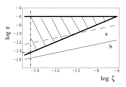
FIG. 1.: Magnetogenesis requirements are illustrated. The thin line b corresponds to $r_{\rm B}(\omega_{\rm G})\sim 10^{-34}$. The dashed line a corresponds $r_{\rm B}(\omega_{\rm G})\sim 10^{-20}$. The (horizontal) thick line correspond to $\epsilon=10^{-6}$. The (diagonal) thick line corresponds to $\epsilon\sim\zeta$. Magnetogenesis is possible when the parameters lie in the shaded area.

To be consistent with inflationary production of scalar and tensor fluctuations of the geometry $\epsilon<10^{-6}$ should be imposed. Thus, in Fig. 1 the parameters should all lie below the (horizontal) thick line. Moreover, since $H_{\rm r}<H_{1}$, $\zeta<\epsilon$. Recall that $\zeta>10^{-15}$ in order not to affect the nucleosynthesis epoch [see the dot-dashed line in Fig. 1]. This requirement comes about since $H_{\rm r}>m$ and $\xi\geq 10^{-15}$.

In this paper the possible phenomenological implications of the evolution of the gauge coupling have been analyzed in the case of a specific model of background evolution. It has been shown that if the gauge coupling is related to a massive scalar field minimally coupled to the geometry the phenomenological constraints related both to the evolution of the massive scalar and to the evolution of the gauge coupling can be satisfied. In a specific example the large scale magnetic fields produced with this mechanism have been computed. It has been shown that they can be large enough to seed the galactic dynamo mechanism. They can be also relevant for the origin of magnetic fields in clusters. Further work on these possibilities is in progress.

Acknowledgments The author wishes to thank M. E. Shaposhnikov for important discussions.

REFERENCES

- [1] P. A. M. Dirac, Nature 139, 323 (1937); Proc. R. Soc. London A 165, 199 (1938); P. Jordan, Z. Phys. 157, 112 (1959); E. Teller, Phys. Rev. 73 , 801 (1948); J. D. Bekenstein, Phys. Rev. D 25, 1527 (1982).
- [2] J. D. Barrow, Phys. Rev. D 35, 1805 (1987).
- [3] T. Appelquist, A. Chodos, and P. G. O. Freund, Modern Kaluza Klein Theories (Addison-Wesley, Redwood City, CA, 1987).
- [4] M. B. Green, J. H. Schwartz, and E. Witten, Superstring Theory (Cambridge University Press, Cambridge, England, 1987).
- [5] P. G. Bergmann, Int. J. Theor. Phys. 1, 25 (1968).
- [6] N. A. Krall and A. W. Trivelpiece, Principles of Plasma Physics (San Francisco Press, San Francisco 1986).
- [7] Smith et al., Phys. Rev. D 61, 022001 (2000); J. C. Long et al., hep-ph/0009062; C. D. Hoyle et al., Phys. Rev. Lett. 86, 1418 (2001).
- [8] G. German and G. G. Ross, Phys. Lett. B 172 305 (1986).
- [9] A. S. Goncharov, A. D. Linde and M. Vysotsky, Phys. Lett. B 147 279 (1993); M. Gasperini, Phys. Lett. B 327, 214 (1994).
- [10] V. A. Kuzmin, V. A. Rubakov and M. E. Shaposhnikov, Phys. Lett. B 155, 36 (1985); V. A. Robakov and M. E. Shaposhnikov, Phys. Usp. 39, 461 (1996) [Usp.Fiz.Nauk 166, 493 (1996)].
- [11] M. E. Shaposhnikov, JETP Lett. 44, 465 (1986); Nucl. Phys. B 287, 757 (1987).
- [12] M. Giovannini and M. Shaposhnikov, Phys. Rev. D 62, 103512 (2000).
- [13] M. Giovannini and M. E. Shaposhnikov, Phys. Rev. D 57, 2186 (1998); Phys. Rev. Lett. 80, 22 (1998); K. Kajantie, M. Laine, J. Peisa, K. Rummukainen, M. E. Shaposhnikov, Nucl.Phys.B 544, 357 (1999); P. Elmfors, K. Enqvist, and K. Kainulainen, Phys.Lett.B 440 269, (1998); M. Giovannini, Phys.Rev.D 61, 063004 (2000); M. Laine, hep-ph/0001292.
- [14] J. B. Rehm and K. Jedamzik, Phys.Rev.Lett. 81, 3307 (1998); H. Kurki-Suonio and E. Sihvola, Phys. Rev. Lett. 84 3756 (2000).
- [15] M. S. Turner and L. M. Widrow, Phys. Rev. D 37, 2734 (1988).
- [16] P. P. Kronberg, Rep. Prog. Phys. 57, 325 (1994).
- [17] T. E. Clarke et al., astro-ph/0011281; H. Bohringer, Rev. Mod. Astron. 8, 295 (1995); K.-T. Kim et al. Astrophys. J. 379, 80 (1991).
- [18] T. Vachaspati and A. Vilenkin, Phys.Rev.Lett. 67, 1057 (1991); B. Ratra, Astrophys. J. Lett. 391, L1 (1992); M. Gasperini, M. Giovannini, and G. Veneziano Phys. Rev. D 52, 6651 (1995); Phys. Rev. Lett. 75 (1995) 3796; M. Giovannini, Phys. Rev. D 56, 3198 (1997); S. Carroll, G. Field and R. Jackiw, Phys. Rev. D 41, 1231 (1990); W. D. Garretson, G. Field and S. Carroll, Phys. Rev. D 46, 5346 (1992); G. B. Field and S. M. Carroll, astro-ph/9811206; A. Dolgov and J. Silk, Phys. Rev. D 47, 3144 (1993); A. Dolgov, Phys.Rev.D 48, 2499 (1993).
- [19] M. Giovannini, Phys. Rev. D 62, 123505 (2000).