Cooling Rates of Molecular Clouds Based on Numerical MHD Turbulence and non-LTE Radiative Transfer

Abstract

We have computed line emission cooling rates for the main cooling species in models of interstellar molecular clouds. The models are based on numerical simulations of super–sonic magneto–hydrodynamic (MHD) turbulence. Non-LTE radiative transfer calculations have been performed to properly account for the complex density and velocity structures in the MHD simulations.

Three models are used. Two of the models are based on MHD simulations with different magnetic field strength (one model is super–Alfvénic, while the other has equipartition of magnetic and kinetic energy). The third model includes the computation of self-gravity (in the super–Alfvénic regime of turbulence). The density and velocity fields in the simulations are determined self–consistently by the dynamics of super–sonic turbulence. The models are intended to represent molecular clouds with linear size $L\approx 6$ pc and mean density $\langle n\rangle\approx 300$ cm^-3, with the density exceeding 10⁴ cm^-3 in the densest cores.

We present ¹²CO, ¹³CO, C¹⁸O, O₂, OI, CI and H₂O cooling rates in isothermal clouds with kinetic temperatures 10–80 K. Analytical approximations are derived for the cooling rates.

The inhomogeneity of the models reduces photon trapping and enhances the cooling in the densest parts of the clouds. Compared with earlier models the cooling rates are less affected by optical depth effects. The main effects come, however, from the density variation since cooling efficiency increases with density. This is very important for the cooling of the clouds as a whole since most cooling is provided by gas with density above the average.

1 Introduction

Line emission by molecules and atomic species is the most important cooling process in interstellar clouds (Goldsmith & Langer, 1978). The temperatures of molecular clouds are determined by the balance between radiative cooling and various heating mechanisms like cosmic ray heating, formation of H₂ molecules, photo-electric heating due to external radiation (de Jong, 1977) and ambipolar drift (Padoan, Zweibel & Nordlund 2000b).

In order to derive the radiative cooling rate for a given species one must first know the excitation conditions in the cloud. However, the cooling rates also depend on the detailed structure of the cloud and the true net flow of energy can only be obtained by solving the full radiative transfer problem. So far the calculations have been based on homogeneous models in different geometries or spherically symmetric clouds with smooth density distribution.

Because of its large abundance the CO molecules is usually the most important coolant of molecular gas. Goldreich & Kwan (1974) studied the CO cooling and made comparisons between the CO cooling rates and the heating associated with cloud collapse. The radiative transfer calculations were based on the Sobolev, or large velocity gradient (LVG), approximation. Goldsmith & Langer (1978) computed cooling rates due to a number of molecules and atomic species using the LVG method applied to spherical, homogeneous and isothermal model clouds. They covered a wide density range up to 10⁷ cm^-3 and a temperatures up to 60 K. Although ¹²CO dominates the cooling of low density gas, the rare CO isotopes, CI and O₂ were found to contribute a large fraction of the total cooling rates. At even higher densities the cooling rates are determined by a large number of species including H₂O, various hydrides and molecular ions. Goldsmith & Langer considered several heating mechanisms and derived equilibrium temperatures for typical clouds.

Neufeld et al. (1995) continued this work by studying radiative cooling rates of dense molecular clouds, $n=$ 10³-10¹⁰ cm^-3 using updated molecular data. The molecular gas was assumed to be fully shielded from external ionizing radiation. Neufeld et al. used chemical models to compute the steady state molecular abundances that were used as the basis of the cooling rate calculations. Level populations of the main cooling species were solved using the escape probability formalism (Neufeld & Kaufman, 1993). Strictly speaking the calculations assume plane-parallel geometry with strong velocity gradient but the results can be applied also to different geometries. That paper concentrated on the study of isothermal, spherical models.

In the present work we re–examine the cooling efficiency of the main cooling agents in molecular clouds at temperatures T${}_{\rm kin}<$100 K. Compared with the earlier studies there are two main improvements: i) The model clouds are no longer assumed to be homogeneous and, more importantly, the density and velocity structures are the result of realistic magnetohydrodynamical simulations; ii) The non-LTE radiative transfer problem is solved exactly with Monte Carlo methods. The solution takes fully into account the inhomogeneous density and velocity fields of the models.

2 The Cloud Models

The numerical models used in this work are based on the results of numerical simulations of highly super–sonic magneto–hydrodynamic (MHD) turbulence, run on a 128³ computational mesh, with periodic boundary conditions.

As in our previous work, the initial density and magnetic fields are uniform. We apply an external random force, to drive the turbulence at a roughly constant rms Mach number of the flow. The force is generated in Fourier space, with power only at small wave numbers ($1\leq k\leq 2$). The isothermal equation of state is used. A description of the numerical code used to solve the MHD equations may be found in Padoan & Nordlund (1999 and references therein).

In order to scale the models to physical units, we use the following empirical Larson type relations, as in our previous works:

$${\cal M}_{s}=4.0\left(\frac{L}{1pc}\right)^{0.5},$$ (1)

where ${\cal M}_{s}$ is the rms sonic Mach number of the flow (the rms flow velocity divided by the sound speed), and a temperature $T=10$ K is assumed, and

$$\langle n\rangle=2.0\times 10^{3}\left(\frac{L}{1pc}\right)^{-1},$$ (2)

where the gas density $n$ is expressed in cm^-3. The rms sonic Mach number is an input parameter of the numerical simulations, and can be used to scale them to physical units. The rms Alfvénic Mach number of the flow ${\cal M}_{a}$ is also an input parameter of the numerical simulations. ${\cal M}_{a}$ is defined as the ratio of the rms flow velocity and the Alfvén velocity, $(\langle B^{2}\rangle/4\pi\langle\rho\rangle)^{\frac{1}{2}}$. It determines the magnetic field strength, once the sonic rms Mach number, ${\cal M}_{s}$, is fixed. We refer to the turbulent flow as super–Alfvénic when ${\cal M}_{a}>1$, while by equipartition turbulence we mean ${\cal M}_{a}\approx 1$.

In this work we use three models. They are all highly super–sonic, with ${\cal M}_{s}\sim 10$. Models $B$ and $C$ are super–Alfvénic, with ${\cal M}_{a}\sim 10$, while model $A$ has rough equipartition of magnetic and kinetic energy of turbulence, with ${\cal M}_{a}\sim 1$. Models $A$ and $B$ neglect the effect of self–gravity, which is instead included in model $C$.

The physical unit of velocity in the code is the isothermal speed of sound, $C_{s}$, and the physical unit of the magnetic field is $C_{s}(4\pi\langle\rho\rangle)^{\frac{1}{2}}$ (cgs). Assuming a kinetic temperature of $T_{\rm kin}$=10 K and a mean density of 320 cm^-3 the mean field strength is $47.0$ $\mu$G in model $A$, $2.2$ $\mu$G in model $B$ and $2.6$ $\mu$G in model $C$. At $T_{\rm kin}$=10 K the rms velocity is approximately 2.1 km/s and the linear size $L=6.3$ pc in all three models. The turbulent velocity inside each computational cell is estimated as the rms velocity between neighboring cells. The macroscopic velocities and the thermal line widths are scaled according to the assumed temperature.

In Figure 1 we show the distribution of cell densities, velocities and magnetic field strength for the three models. Model $B$ has the widest range of densities and the largest fraction of dense cells, $n\sim$10³ cm^-3 (top panel of Figure 1). In $C$ the density distribution is skewed towards lower densities. Model $A$ is the least inhomogeneous one, but the density contrast is still larger than three orders of magnitude. As can be seen from the middle panel of Figure 1, differences in the velocity distribution between different models are insignificant. The magnetic field strengths are shown in the bottom panel of Figure 1, with physical values obtained for the mean density $n=320$ cm^-3 and the kinetic temperature $T_{\rm kin}=20$ K.

Figure 1: Number of cells in the three model clouds ($A$, $B$ and $C$) as a function of density (a) velocity (b) and magnetic field strength (c). The plots assume a mean density of 320 cm^-3 and a temperature of $T_{\rm kin}$=20 K.

3 The Calculation of the Cooling Rate

The cooling rates are calculated individually for each cell in the model clouds and for several cooling species. The original MHD simulations were performed on a 128³ grid but because of the high computational burden of the radiative transfer calculations most of these calculations were carried out with model clouds re-sampled into a 90³ cell grid. The discretization introduces some small smoothing of the high density peaks but is otherwise not expected to affect the derived cooling rates.

The collisional coefficients for CO were taken from Flower & Launay (1985), CI-H₂ rates are from Schröder et al. (1991) and OI-H₂ rates from Jacquet et al (1992). The rate coefficients for collisions O₂-H₂ and O₂-He were provided by P. Bergman (1995; private communication).

3.1 Fractional Abundances of the Cooling Species

The cooling rates are calculated for the species ¹²CO, ¹³CO, C¹⁸O, O₂, CI and OI. According to Neufeld & Kaufman (1993) these are the most important cooling species in the present parameter region, that is at densities below $\sim 10^{4}$ cm^-3 and at temperatures $T_{\rm kin}<$100 K. Cooling rates due to H₂O are calculated only at T_kin=60 K.

For the CO species we assume fractional abundances [¹²CO]/[H₂]=$5\cdot 10^{-5}$, [¹³CO]/[H₂]=$1\cdot 10^{-6}$ and [C¹⁸O]/[H₂]=$1\cdot 10^{-7}$. These values are similar to those adopted by Goldsmith & Langer (1978). The CO abundance is lower than predicted by standard chemical models (Millar et al., 1997; Lee et al., 1997) but consistent with observation (e.g. Ohishi et al. 1992) which also show a significant variations between clouds (Harjunpää & Mattila, 1996). Depending e.g. on the radiation field and the gas temperature, chemical fractionation can lead to abundance variations (e.g. Warin et al. 1996) but we shall assume constant abundances throughout the clouds. This is probably a good approximation since the inhomogeneous density distribution reduces differences in the radiation field between inner and outer parts of the cloud (Boissé, 1990; Spaans, 1996) and we do consider only isothermal models.

The abundances of O₂ and OI are not well known. Recent results from the ISO and SWAS satellites show that the oxygen abundances in molecular clouds have been previously overestimated and probable values are below [O₂]/[H₂]$\sim 10^{-6}$ (Bergin et al., 2000; Goldsmith et al., 2000). On the other hand, Caux et al. (1999) found L1689N to be rich in OI indicating that the abundance of OI can be as high as [OI]/[H₂]$\gtrsim 10^{-5}$. The predictions of chemical models have usually been closer to 10^-4 for both [OI]/[H₂] and [O₂]/[H₂] (e.g. Lee et al. 1997). Above 100 K the abundances are also very sensitive to the assumed temperature but in the temperature range considered in the present work the abundances are essentially independent of temperature (Neufeld et al., 1995). We use an abundance of $10^{-5}$ for both OI and O₂. In view of the recent observational results the OI abundance is adequate but the O₂ abundance might be too high by more than one order of magnitude. However, a similar value is used by Goldsmith & Langer (1978) and Neufeld et al. (1995), which makes comparison with their results easier. For CI a fractional abundance value of 10^-6 will be used.

For water a fractional abundance of 1.0$\cdot 10^{-6}$ is assumed. Calculations are carried out separately for ortho- and para-water with ortho to para ratio 1:3. The total abundance is similar to the values used by Goldsmith & Langer (1978) and Neufeld et al. (1995). However, observations of quiescent gas in molecular cloud cores, Orion and M17SW (Snell et al., 2000a, b, c) have indicated much lower abundances [H₂O]/[H₂]$\sim 10^{-8}$. Similar values have been reported by Ashby et al. (2000). The lower values would mean that water is unimportant for the cooling of the clouds considered here. Locally H₂O can be very efficient coolant since in outflows and hot cores its abundance can be enhanced up to [H₂O]/[H₂]$\sim 10^{-4}$ (Snell et al., 2000c) and the importance of H₂O increases with temperature. Our models represent, however, relatively cold and quiescent clouds. The H₂O cooling rates are therefore computed only for $T_{\rm kin}$=60 K and with relative abundance [H₂O]/[H₂]=1.0$\cdot 10^{-6}$ the results can be taken as upper limits for the actual H₂O cooling.

Since we will examine only isothermal models, the possible temperature dependence of the abundances affects only the comparison between models with different $T_{\rm kin}$. At these low temperatures the temperature dependence is, however, weak. According to models (e.g. Lee et al. 1997) there can be a significant dependence on the gas density even when photo-processes due to external radiation field are not considered. The effect is especially clear for carbon. In the standard model presented by Lee et al. (1997) the carbon abundance increases by a factor $\sim$10 as the gas density decreases from 10⁴ cm^-3 to 10³ cm^-3. This would reduce the spatial variation in the carbon emission. We have not included these abundance variations in our models. The steady state abundances are not necessarily valid for the turbulent medium of the MHD models where density variations are caused by moving shock fronts and the predicted abundances must be treated with some caution.

3.2 Energy Levels Used in the Calculations

For practical reasons the number of energy levels that can be included in the calculations is limited. The number of levels needed for an accurate estimate of the cooling rate depends mainly on the excitation as all significantly populated levels must be considered. The relative importance of the transitions is affected also by optical depth, as optically thick transitions contribute less to the total cooling rate.

In the case of ¹²CO we find that at low temperatures, $T_{\rm kin}\leq 20$ K, it is sufficient to include levels up to $J=11$. Higher transitions are more important at higher densities. However, at 20 K, the cooling rate of the $J=8-7$ transition is approximately two orders of magnitude below that of the $J=2-1$ transition, even for densities $n\gtrsim$10³ cm^-3. The total contribution from higher transitions is insignificant.

At higher temperatures, $T_{\rm kin}>20$ K, we include the 15 lowest energy levels of ¹²CO. In Figure 2 the cooling rate in model $B$ is plotted as a function of the kinetic temperature. At $T_{\rm kin}\geq 60$ K and at densities $n\sim$10⁴ cm^-3 the cooling rate from the $J=8-7$ transition is roughly equal to the rate from the $J=2-1$ transition. However, the population as a function of $J$ decreases rapidly and the contribution of levels close to $J=14$ is insignificant. All models have similar ranges of density and the same number of levels is used also for the other two model clouds ($A$ and $C$).

Due to small optical depths the number of populated ¹³CO and C¹⁸O levels is lower than in ¹²CO. For these species we include 10 levels at $T_{\rm kin}\leq$20 K and 12 at higher temperatures. The number of O₂ levels used in the calculations was the same as for CO but because of the fine structure there are now 22 transitions between the first 15 energy levels. For both CI and OI, 3 energy levels were used, with only 2 transitions between them. The CI lines are ³P₁-³P₀ at 610 $\mu$m and ³P₂-³P₀ at 230 $\mu$m and the corresponding OI lines are at 145 $\mu$m and 63 $\mu$m. Cooling rates due to H₂O were calculated only at 60 K and only 11 energy levels (20 transitions) were included. This is adequate due to the relatively low densities and temperatures. The highest included levels are more than $400$ K above the ground state and are not significantly populated.

The inhomogeneous cloud structure of the MHD models increases the photon escape probability in otherwise optically thick transitions. The cooling rate from lower transitions is increased while the population of the higher levels is decreased.

Figure 2: The cooling rates, $\Lambda/n$, due to selected ¹²CO transitions ($J=$2-1, 4-3, 6-5 and 8-7) as a function of the kinetic temperature. The rates are averaged over cells in the density ranges 10³-10⁴ cm^-3 (upper panel) and 10-10² cm^-3 (lower panel). The errorbars correspond to the dispersions within the given density ranges.

4 The Radiative Transfer Method

The model cloud is divided into 90³ cells. Each cell is assumed to be homogeneous and is characterized by one value of density, intrinsic linewidth and macroscopic velocity. Density and velocity are obtained directly from MHD simulations once the results are scaled to physical units. The intrinsic linewidth is the sum of thermal line broadening and the Doppler broadening caused by turbulent motions inside the cell. The latter is estimated as the rms velocity difference between neighboring cells. The components are of the same order but usually the turbulent line broadening is the larger of the two.

The radiative transfer problem is solved with a Monte Carlo method (method B in Juvela 1997). The radiation field is simulated by a large number of photon packages going through the cloud. These represent both photons entering the cloud from the background and photons emitted within the cloud. As a photon package goes through a cell the number of photons absorbed within that cell is removed from the package. At the same time the number of upward transitions induced by these photons is stored in counters. There is a separate counter for each cell and each simulated transition. After the simulation of the radiation field the counters are used to obtain new estimates of the level populations. The whole process is repeated until the level populations converge (the relative change from an iteration to the next is less than 10^-4). The core saturation method was used to speed the calculations of optically thick species (Hartstein & Liseau, 1998; Juvela & Padoan, 1999).

The cooling rates of the cells are also calculated with a Monte Carlo method, using the previously obtained level populations. During the computation the net flux of photons is counted for each cell and this is transformed into cooling rates in units of erg s^-1 cm^-3. In order to study the relative importance of the transitions the net flux is counted for each transition separately.

Figure 3: Distributions of effective hydrogen column density, N_eff, in the three model clouds. The average density is 320 cm^-3 and the linear size 6.3 pc in all models.

5 Results

5.1 Cooling Rates

The local cooling rate depends mainly on three parameters: the local density, kinetic temperature and effective column density, or effective optical depth. The optical depth determines the photon escape probability that in our case is strongly affected by the inhomogeneity of the clouds. The optical depth seen by a cell varies strongly depending on the line of sight. This is true throughout the cloud, not only close to the cloud surface. The effective optical depth depends on both the density and the velocity distributions since the velocity dispersion is always large compared with the thermal linewidth. The velocity dispersion in the models is approximately 3.0 km/s, assuming a sound speed 0.3 km/s.

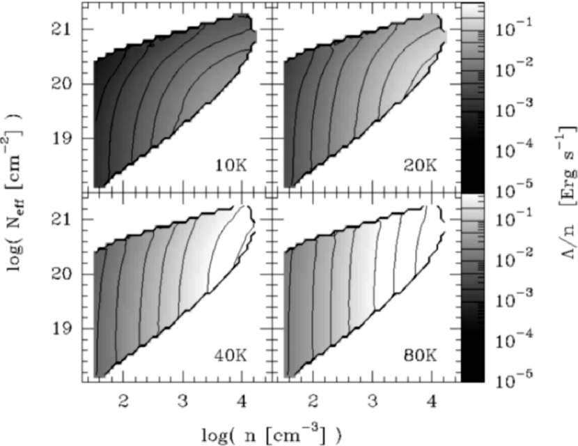
Figure 4: ¹²CO cooling rates $\Lambda/n$ as a function of density, $n$, and effective column density, $N_{\rm eff}$, in model $B$.

In order to quantify these effects, we have calculated the effective column density, $N_{\rm eff}$, seen by each cell in the three models. We define this as

$$N_{\rm eff}\,\,=\,\,\langle\,\,\left(\int N(v)\phi(v)dv\right)^{-1}\,\,\rangle^{-1}.$$ (3)

$N(v)$ is the column density along one line of sight from the edge of the cloud to the cell and $\phi(v)$ is the local absorption profile, both given in units of velocity. The integral is proportional to the column density seen by the cell towards one direction and the averaging is done over all directions. $N_{\rm eff}$ is calculated as a by-product of the radiative transfer calculations. The cooling rate depends on $N_{\rm eff}$ through its effect on the effective optical depth seen by the cells i.e. the escape probability. The optical depth depends in a complicated way on the excitation in other parts of the cloud. The effective column density is, on the other hand, a parameter of the cloud itself and describes the effects of the density and velocity fields independently of the studied molecule. For these reason the effective column density will be used as a substitute for the effective optical depth.

The distributions of $N_{\rm eff}$ seen by individual cells are shown in Figure 3 for the three models. $N_{\rm eff}$ is smallest on the surface of the cloud and increases towards the centre depending, however, on the actual density and velocity fields. In microturbulent case with gaussian line profiles we would get $N_{\rm eff}=N/\sqrt{4\pi\,\sigma^{2}}$. Here $N$ is approximately equal to the average column density between the cell and the cloud boundary. In our case we have $<n>=320$ cm^-3 and $L/2$=3.1 pc. When total velocity dispersion, some 3 km s^-1 at 20 K, is used for $\sigma$ we obtain an effective column density of $\sim$3$\cdot$10²⁰cm^-2 km^-1 s in the cloud centre. In MHD simulations the turbulence is, however, not random and more importantly the density distribution is not constant. Higher values, up to $N_{\rm eff}\sim 10^{21}$cm^-2 km^-1 s, are therefore reached in dense and velocity coherent regions.

Figure 4 summarizes the CO cooling rate for model $B$ as a function of density, $n$, effective column density, $N_{\rm eff}$, and temperature. In Figure 5 the cooling rate $\Lambda({\rm CO})/n$ in model $B$ is plotted as a function of the effective column density $N_{\rm eff}$, for different density intervals and kinetic temperatures $T_{\rm kin}$. This illustrates some basic features seen in the case of all three model clouds.

Figure 5: Cooling rate $\Lambda({\rm CO})/n$ in model $B$ as a function of the effective column density $N_{\rm eff}$, in clouds with kinetic temperature T_kin=10, 20 or 60 K. Each panel shows the average cooling rates in three density intervals, 2.2-4.2$\cdot$10¹ cm^-3 (lowest curves), 2.2$\cdot$10²-4.2$\cdot$10² cm^-3 and 2.2$\cdot$10³-4.2$\cdot$10³ cm^-3 (highest curves). The errorbars reflect the variation of $\Lambda({\rm CO})/n$ in the given density intervals.

$\Lambda/n$ decreases with $N_{\rm eff}$, particularly in the case of low temperatures and high volume densities. The behavior is the result of the dense cores becoming opaque. In low density regions, the net cooling is reduced also by the incoming flux from surrounding regions that, due to the higher density, have higher excitation temperature. At higher kinetic temperatures more transitions are contributing to the cooling rates and photon trapping cannot reduce the cooling rates to the same extent.

Similar effects can be seen by studying the cooling rates $\Lambda/n$ computed separately for different CO transitions. Figure 6 illustrates the situation for model $B$. The increasing importance of higher CO transitions with increasing column density is evident. In the higher density ranges the importance of higher transitions is larger (see Figure 6). The increase in the cooling rate of the $J=6-5$ transition, for example, tends to be more rapid than the decrease in lower transitions. As a result, the total cooling rate does not drop significantly with $N_{\rm eff}$.

Figure 6: Cooling rate $\Lambda({\rm CO})/n$ from different CO transitions in model $B$, as a function of the effective column density $N_{\rm eff}$. The kinetic temperature is $T_{\rm kin}$=20 K. The panels correspond to the density ranges: 2.2$\cdot$10¹-4.2$\cdot$10¹ cm^-3 (a), 2.2$\cdot$10²-4.2$\cdot$10² cm^-3 (b) and 2.2$\cdot$10³-4.2$\cdot$10³ cm^-3 (c). The variation in the cooling rates within the given density intervals is indicated by errorbars.

Figure 7: Cooling rate $\Lambda({\rm CO})/n$ from different CO transitions in model $B$, as a function of the effective column density $N_{\rm eff}$ at three temperatures, $T_{\rm kin}$=10 K (top panel), 20 K (middle panel) and 60 K (bottom panel). The curves represent the average rate for the density interval 2.2$\cdot$10²-4.2$\cdot$10² cm^-3.

Figure 7 shows similar $\Lambda/n$ dependencies at three temperatures. At $T_{\rm kin}=10$ K the cooling rate of the transition $J=2-1$ (and $J=1-0$) decreases strongly as column density exceeds $10^{20}$ cm^-2. The increase in the cooling rate from the higher transitions is unable to compensate for the loss and the total cooling rate decreases as seen in Fig 5. On the other hand, already at $T_{\rm kin}$=20 K the cooling rate by the transition $J=4-3$ exceeds at high column densities that of the transition $J=2-1$ and $\Lambda/n$ levels off. However, the rates do not decrease significantly even at $N_{\rm eff}=5\cdot 10^{20}$ cm^-2. At $T_{\rm kin}$=20 K the average optical depths averaged over the whole cloud are $\tau(J=2-1)\approx 130$, $\tau(J=4-3)\approx 65$ and $\tau(J=6-5)\approx 0.5$. At 60 K the corresponding values are $\tau(J=2-1)\approx 30$, $\tau(J=4-3)\approx 42$, $\tau(J=6-5)\approx 11$ and $\tau(J=8-7)\approx 0.4$. At higher temperatures optical depths of individual transitions are lower and this reduces the effect that column density has on local cooling rates.

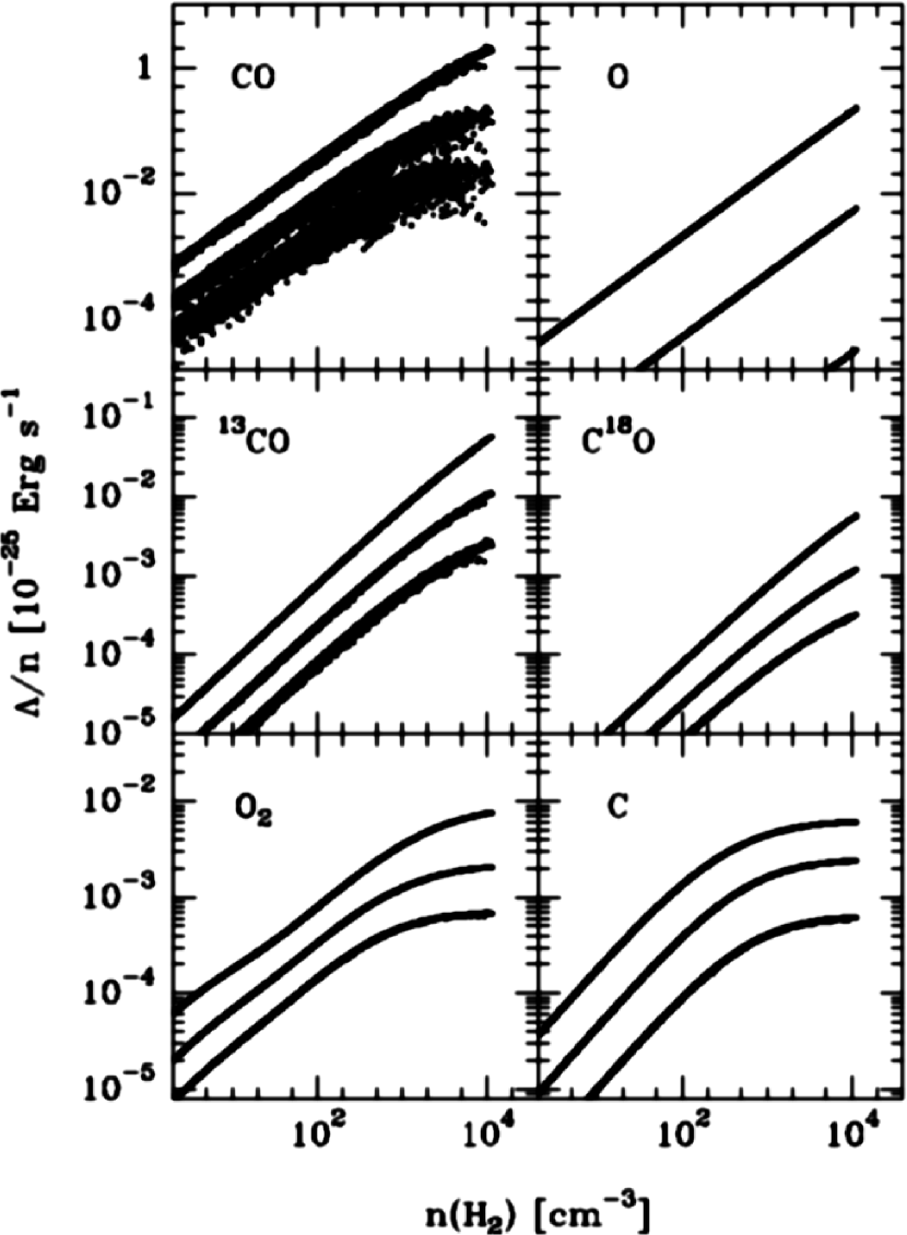
Figure 8: The cooling rate $\Lambda/n$ in the cells of model $B$ as a function of local gas density. The curves correspond to different values of the kinetic temperature, $T_{\rm kin}$=10, 20, and 60 K, in increasing order. Rates are plotted for every tenth cell in the model.

Figure 9: Parameters of Eq. 4 as a function of the kinetic temperature of the model, $T_{\rm kin}$, when fitted to the ¹²CO cooling rates $\Lambda({\rm CO})/n$. The panels correspond to the three cloud models $A$, $B$ and $C$.

5.2 Analytic Approximations

We have computed an analytic approximation of the cooling rates $\Lambda=\Lambda(n,T_{\rm kin},N_{\rm eff}$). The rates $\Lambda/n$ are fitted at each temperature with a function

$$f(n,N_{\rm eff}) = a\times$$ (4)

$$(1+b\,log({n\over 10^{3}})+c\,(log({n\over 10^{3}})^{2}))\times$$

$$(1+d\,log({N_{\rm eff}\over 10^{20}})+e\,(log({N_{\rm eff}\over 10^{20}}))^{2})$$

$$= log\,\Lambda/n\,[10^{-25}\,{\rm erg}\,{\rm s}^{-1}]$$

This is not the most optimal functional form for fitting the cooling rates but is conceptually simple. Parameters $b$ and $d$ are, respectively, the slopes of the density and the column density dependence and the parameters $c$ and $e$ represent the non-linearity of these relationships. As a first approximation the dependence of the $\Lambda/n$ on the density and column density is linear on the log-log scale. Deviations from this behavior are visible at low kinetic temperatures as a flattening or even a turnover in the density dependence. Although similar turnover is seen in the cooling rates of individual CO transitions also at higher temperatures (see Figure 8) the total cooling rates are monotonic in the present density and column density ranges. The turnover is simply transferred to higher densities and/or column densities. In the case of CI, flattening is even more pronounced and persists to higher temperatures.

For the fitting of Eq. 4 the cells of the clouds were divided into small density and column density bins and the parameters of Eq. 4 were fitted using the average values $\langle n\rangle$, $\langle N_{\rm eff}\rangle$ and $\langle\Lambda\rangle$ in each bin. The fitting was weighted with the number of the cells in each bin and the fit is therefore least reliable in the tails of the density and column density distributions.

Figure 9 shows the fitted parameters as a function of the kinetic temperature in the case of ¹²CO. Note the decreasing dependence of cooling rate on column density when kinetic temperature is increased (coefficients $d$ and $e$). As already stated, this is a natural consequence of the reduced optical depth per transition. A related effect is the increased importance of density at higher temperatures (coefficients $b$ and $c$). The first excitation level of CO is at $\sim$5 K and e.g. $J=5$ is $\sim 80$ K above the ground state. Therefore, at $T_{\rm kin}\sim$10 K only a couple of levels can be populated whereas at $T_{\rm kin}\sim$80K̇ a density increase can easily double the number of populated levels and markedly increase the escape probability of the emitted photons.

Figure 10: Cooling rate, $\Lambda/n$, of the studied species as a function of the gas density in model $B$. The lower panel corresponds to kinetic temperature $T_{\rm kin}$=20 K; the upper panel to $T_{\rm kin}$=60 K. The rates for CI are drawn with dashed lines. At 60 K the sum of the computed ortho-H₂O and para-H₂O rates is shown as a dotted line. With the abundances used in this paper the O₂ rates (not shown) would be roughly equal with the CI rates. As the real O₂ abundances are expected to be much lower its contribution to the cooling will be negligible

The dependence on the effective column density, $N_{\rm eff}$, is not very strong for the cooling rate $\Lambda/n$. This is true for optically thin species and even for ¹²CO, at least for temperatures above 10 K (see Figure 5). It is therefore reasonable to search for an analytical approximation for $\Lambda/n$ as a function of density and kinetic temperature alone. The function

$$\log{(\Lambda/n)}=c_{1}\sqrt{\log{T}}+({\log{n}})^{3/2}\left(c_{2}+c_{3}/\sqrt{\log{T}}\right)$$ (5)

may be used to represent the ¹²CO and the total cooling rate with $\sim$20% accuracy over the studied density and temperature ranges, where the absolute values of $\Lambda/n$ change by more than a factor of 10⁴. The parameter values obtained for the fits to total cooling rates are listed in Table 1.

Table 1: Parameters of Eq. 5 obtained by fitting the cooling rate, $\Lambda/n$ [$10^{-25}$ erg s^-1], in the three models. The equation  5 gives the local cooling rate as a function of local gas density and the kinetic temperature.

model	c1	c2	c3
$A$	-4.23	0.80	-0.121
$B$	-4.14	0.78	-0.118
$C$	-4.24	0.82	-0.129

6 Discussion

In the parameter range studied ¹²CO is the main coolant. In Figure 10 we plot the cooling rates from model $B$ as a function of the gas density, for all the coolants included in our study. The most important difference between $T_{\rm kin}$=20 K and 60 K is the increased cooling from O at the higher temperature, where it provides $\approx 10$% of the total cooling rate. Due to the lower optical depth per transition the ¹²CO cooling rate is, at 60 K, considerably higher than the cooling rate of ¹³CO and C¹⁸O. The sum of the computed para-H₂O and ortho-H₂O rates are shown for $T_{\rm kin}$=60 K. At this temperature the contribution from H₂O is not very significant.

According to Neufeld et al. (1995) the most important group of coolants not included in our calculations is the non-hydride molecules. Neufeld et al. estimate the total effect from these using the formula

$$L= \sum_{diatomic}L_{\rm CO}(0.01\,n,100\,\tilde{N})$$ (6)

$$+\sum_{polyatomic}L_{\rm CO}(0.008\,n,7\,\tilde{N})$$

with $L(\rm M)$ defined as $\Lambda=L\,n({\rm H}_{2})n({\rm M})$ for each species M. According to the formula the rates are similar to those of CO in gas with lower volume density and higher column density. The average dipole moment of diatomic non-hydrides (CS, NO, CN etc.) is approximately 10 times the dipole moment of the CO molecule. The radiative rates are therefore two orders of magnitude higher and this results in the first term of the equation. The second term for polyatomic non-hydrides was based on the computed cooling function of SO₂ (see Neufeld et al. 1995).

Using the CO cooling functions derived in this work, substituting $N_{\rm eff}$ for $\tilde{N}$ in Eq. 6 and using the steady state fractional abundances published by Lee et al. (1997), ‘new standard model’, $T_{\rm kin}$=10 K, $n$=10³ cm^-3, we can estimate the contribution from these other molecules. With the CO cooling function fitted in model $B$ we find that at $T$=10 K this amounts to $\sim$10% of the CO cooling rates at the high density limit of our models, $n$=$10^{4}$ cm^-3. The importance of these other molecules decreases rapidly with decreasing density. The cooling rate decreases also with increasing kinetic temperature so that at 60 K it is less than 5% of the CO cooling rate.

Although the previous estimates are very crude we can conclude that for our models the non-hydride molecules are not important, except perhaps in the densest and coldest cores, where they could provide $\approx 10$% of the total cooling. However, this number is uncertain and can be altered significantly, for example by assuming different fractional abundances.

6.1 Comparison Between MHD Models

Both density and velocity fields are important in determining the cooling rate of optically thick lines. We may therefore expect to see some differences between the MHD models although they are similarly inhomogeneous in both density and velocity space.

Compared with the model $B$ at $T_{\rm kin}$=10 K the average cooling rate, $\lambda/n$, is $\sim$15% lower in model $A$. The difference increases with temperature and exceeds 30% at $T_{\rm kin}$=60 K. The difference is, however, partly due to the fact that model $B$ has more high density cells with correspondingly higher cooling rates (see Figure 1a). In fact, for densities below 10³ cm^-3 the cooling efficiency is higher in model $A$. At column density $N_{\rm eff}\approx$10²⁰ cm^-2 and volume density 10² cm^-3 the cooling rates ($\lambda/n$) in model $A$ are a few of percent larger than in model $B$. At somewhat higher densities, $n\approx 3\cdot$10³ cm^-3, the rates are below those of the model $B$ (at 10 K by some 10% but at 60 K by only $\sim$1%).

The net cooling rate ($\Lambda/n$) in model $C$ is 4% smaller than in model $B$. As a function of density and column density the rates are between those of the models $A$ and $B$ and usually closer to the rates in model $A$. The model $C$ included self-gravity which should affect the structure of the high density concentrations. This does not, however, show clearly in the overall density distribution (see Figure 1) and even at $n\sim$10³ cm^-3 the cooling rates are quite similar to those found in the other models. Same trend continues up to highest densities, $n\sim$10⁴ cm^-3, with model $B$ having cooling rates 5-10 % in excess of the other two models.

The cooling function should be sensitive to the cloud structure. In the range $n=$10¹–10³ cm^-3 and $N=$10¹⁹–10²¹ cm^-2 the differences in the ¹²CO cooling efficiency in the three MHD models are, however, below 20% and from this point of view the models do not differ radically from each other. All have similar types of inhomogeneous density structures and the overall velocity dispersions are also similar. Furthermore, the clumpiness increases the photon escape probability and reduces any effects caused by large optical depths. The differences between MHD models would be enhanced e.g. in clouds with larger size, higher density or lower turbulence.

6.2 Average cooling rates

In the previous chapters we have studied the local cooling rate as a function of the local gas properties, density $n$ and kinetic temperature $T_{\rm kin}$, and the general environment described by the effective column density $N_{\rm eff}$. Since earlier theoretical studies and observers tend to concentrate on the average properties of the clouds we will now discuss the average cooling rate which is also proportional to the net cooling of the cloud as a whole.

Figure 11: The cooling rates averaged over model $B$, as a function of the kinetic temperature of the model. The mean density is $<n>$=320 cm^-3.

Figure 11 shows the cooling rates in model $B$ averaged over the model volume. Note the steep temperature dependence of the OI emission. The actual ratios between different species depend on the assumed abundances and, as already mentioned, for species other than ¹²CO the cooling efficiency scales almost linearly with the abundance.

We now study more closely the ¹²CO cooling. The cooling rate depends strongly on the density (Figure 8). In an inhomogeneous cloud this means that most of the cooling power comes from regions denser than the average. The average cooling rate is also higher than the local rate at the density equal to the mean density of the cloud. This is true as long as the dense cores are not optically very thick. When the cores become opaque to most of the cooling lines the cooling efficiency will not increase any more with increasing density and the total cooling efficiency will be reduced.

Figure 12: The ¹²CO cooling in model $B$ at three kinetic temperatures. The longer curves show the local cooling rates as a function of the local gas density. The mean density of the model was 320 cm^-3. The filled squares show the cooling rates averaged over the model, as a function of the mean density of the model. The models were obtained by scaling the mean density of model $B$ to 160, 320, 640, 1280 and 2560 cm^-3

Figure 12 shows both the local cooling rate and the average cooling rate of ¹²CO, as a function of density for three different kinetic temperatures. The local rates are obtained from the individual cells of the model $B$ as the cooling rate of a cell divided by the gas density in the cell. The entire model cloud provides the point at 320 cm^-3 for the curve showing the average cooling rate $<\Lambda>/<n>$. Here the cooling rate and the density are averaged separately over the volume of the model. The average cooling rate is proportional to the net cooling rate of the entire model (erg s^-1). Other points for the average cooling rate are from models which were obtained by scaling the mean density of model $B$ to 160, 640, 1280 and 2560 cm^-3.

The rates follow the expected behavior outlined above. At lower densities the average rates exceed the local rates, with a ratio approaching a factor of ten. Even in the $<n>$=320 cm^-3 model the CO rate $\Lambda/n$ levels off at the highest densities. In models with high mean density this leads to a turnover and eventually the average rate drops below the curve for the local cooling rate. This means that gas below the mean density is getting more and more important for the net cooling of the cloud. For 10 K models the curves meet below 10³ cm^-3. At higher temperatures the optical depth effects are again reduced and at 60 K the average rate remains above the local rate until close to 10⁴ cm^-3. This is perhaps the most striking result of the present work. Molecular clouds described by turbulent density and velocity field as modeled here, can radiate 10 times more efficiently than a uniform cloud with density equal to the mean density of our model. As a consequence, their thermal balance requires a ten times larger heating source.

In order to study separately the effects of the density and the velocity inhomogeneities we have considered two further models that are based on model $B$. The constant density model, $CD$, has constant density 320 cm^-3 (equal to the mean density in the model $B$) but the velocity structure of the model $B$. The constant velocity model, $CV$, has the same density structure as the model $B$ but no macroscopic velocity field. Only ¹²CO cooling rates were calculated since, due to high optical depth, these are most likely to show differences between the models.

Compared with model $B$ the effective column densities are higher in $CV$ and $CD$, since the inhomogeneity of either densities or velocities is removed. This gives the appearance of increased $\Lambda/n$ when plotted against $N_{\rm eff}$. This is, however, only due to the shift of the $N_{\rm eff}$ axis and the total cooling rate of the clouds is reduced. This is natural since the escape probability of emitted photons is smaller. For model $CV$ the total ¹²CO cooling rate is reduced by $\sim$10% at $T_{\rm kin}$=10 K. The effect reduces at higher temperatures as the optical depths of individual transitions are reduced. For model $CD$ the drop is $\sim$50% at 10 K and increases with temperature. The difference between the original model and $CD$ is not due to radiative transfer effects but is rather a direct consequence of the steep density dependence of the cooling function. In an inhomogeneous cloud most of the cooling is provided by regions with density well above the average value. For optically thin emission the ratio of average cooling rate and cooling rate at the mean density can be derived directly based on the cell density distribution (Figure 1) and the density dependence $\Lambda\sim n^{2}$. The ratios are 3.9, 8.0 and 8.9 for the models $A$, $B$ and $C$, respectively.

Since density peaks are very important for the cooling we must make sure that the results are not affected by the limited spatial resolution. The CO cooling rates were compared in three variants of the model $B$ where the cloud was divided into either 128³, 90³ or 48³ cells. The plots of local cooling rates against local density were almost indistinguishable although at lower resolutions the total range of densities was reduced. A change in the discretization causes changes in the cell densities. In the plot this means only a small displacement along the $\Lambda(n)$ curve which itself remains unchanged. As the cell size is increased some of the velocity dispersion between cells (‘macroturbulence’) is transformed into turbulent velocity inside the cells (‘microturbulence’) but this did not produce any noticeable effects on the cooling rates. At $T_{\rm kin}$=20 K the total cooling rates of the models were within $\sim$3% of each other. This shows that the selected resolution was sufficient to capture the effects of density and velocity inhomogeneities. Our models represent quiescent diffuse clouds. In models with more developed cloud cores and steeper density gradients the spatial resolution should be correspondingly higher.

6.3 Comparison with Earlier Work

Most previous calculations of molecular line cooling rates have focused on specific objects (for example dense cores) and are therefore not useful for comparison with the present work. In particular, little has so far been published on the subject in connection with inhomogeneous clouds. In the following we look at some of the differences between our work and the results obtained by Goldsmith & Langer (1978) and Neufeld et al. (1995). Their results apply to clouds with continuous and smooth density distributions. Differences will be caused by two factors. Firstly, our MHD models contain a range of densities and due to steep density dependence (e.g. Figure 8) total radiated energy will be larger than in a homogeneous cloud with equal mean density (see previous chapter). Secondly, excitation and escape probability of emitted photons will be affected by the density and velocity inhomogeneities.

Figure 13: Comparison of our ¹²CO and CI cooling rates with Goldsmith & Langer (1978). The solid curves show our local cooling rates in model $B$ as a function of the local gas density. The errorbars indicate the variation within the density bins. The solid squares show our estimates for the average cooling as a function of the average density of the model cloud (see text). The dashed curves are ¹²CO and CI rates taken from Goldsmith & Langer (1978)

In Figure 13 we plot the Goldsmith & Langer (1978) cooling rates for ¹²CO and CI together with our average rates at a few densities (solid squares). In the same figure the local cooling rates for the $n=320$ cm^-3 model are also shown (solid curve). This should be compared only with those points on the other curves that correspond to the same density.

We will first compare the CO rates. For the LVG model used by Goldsmith & Langer the relevant parameter is the CO abundance divided by the velocity gradient, $X_{\rm CO}/\,(dV/dr)$. In our models a corresponding parameter can be calculated using the average velocity dispersion of the cloud and the linear size of the model, $L$. Choosing models where these parameters agree ensures that the average properties of the LVG and the MHD models will be similar. Differences will be caused by differences at smaller scales i.e. mostly by the density and velocity inhomogeneity of our models. In the MHD simulations the velocity and density fields are not completely random and depending on the line of sight the average density and column density can differ significantly from the values averaged over the entire volume of the cloud.

In the following we will use the FWHM of the one-dimensional velocity distribution as the measure of the velocity dispersion in our models. The value is calculated as the average over the whole cloud. In model $B$ the FWHM of the velocity dispersion is 2.90 km s^-1 at $T_{\rm kin}$=10 K. With abundance 5$\cdot$10^-5 and cloud size 6.25 pc we get a column density per velocity unit of 1.08$\cdot$10^-4 pc km^-1s. In Figure 13 the model is compared with Goldsmith & Langer calculations for $X/\,(dV/dr)$=10^-4 pc km^-1s. At 40 K the velocity dispersion in the MHD model was higher, FWHM=5.77 km s^-1, corresponding to the higher speed of sound. The column density is 5.4$\cdot$10^-5 pc km^-1s and the corresponding value of the Goldsmith & Langer model shown in Figure 13 is 4$\cdot$10^-5 pc km^-1s. Goldsmith & Langer note that their results are not sensitive to the assumed velocity gradient and in our case similar conclusion can be drawn from the weak column density dependence in Figure 5. Therefore, an absolute equality of the column density parameters is not crucial and the qualitative result of the comparison would remain the same even if our column density values were scaled by a factor of two.

At 10 K our local  ¹²CO cooling rate at $n=$320 cm^-3 agrees with the predictions of Goldsmith & Langer (see Figure 13). The point is still on the linear portion of the curve i.e. radiative trapping is not yet significant. The average cooling rate is, however, two times higher than either the Goldsmith & Langer value or our local cooling rate at that density. This is due to the fact that the density dependence of the cooling rate $\Lambda$ is steeper than $n^{1.0}$. In the case of a wider distribution of density values the average cooling rate increases even when the mean density remains unaltered.

At 40 K the effects of optical depth are greatly reduced and in the model with mean density 320 cm^-3 the local cooling rate is almost a linear function of local density. This increases the difference to Goldsmith & Langer results which are at $n=10^{4}$ cm^-3 a factor of six below our rate. At 10 K the average cooling rate $\Lambda/n$ was a decreasing function of density but at 40 K it increases up to $<n>\sim 10^{3}$cm^-3. In the model with mean density $<n>$=320 cm^-3 the local cooling rate exceeds the volume averaged rate by a factor of four.

In Figure 13 the errorbars indicate the variation in local cooling rate, $\Lambda/n$, within each density bin (see also Figure 8). Although this does include some noise from the Monte Carlo calculations most of the variation is due to radiative transfer effects. The cells are in different environments (e.g. cloud centre vs. cloud surface) and this affects the cooling. At 40 K the local cooling rate is rather uniform while at 10 K there is wider scatter, especially at high densities. This shows again how an increasing kinetic temperature reduces the effects of optical depth.

For CI the abundance used in this paper was 10^-6 i.e. a factor of ten lower than the value used by Goldsmith & Langer. The relevant parameter is, however, again $X_{\rm CI}/\,(dV/dr)$. None of the results published by Goldsmith & Langer correspond exactly to the parameters of our models and therefore we have rescaled our abundance value so that our model can be compared directly with their Figure 7. Another difference is caused by the collisional coefficients. Goldsmith & Langer used for CI-H₂ collisions the Launay & Roueff (1977) CI–H rates divided by ten. In this paper we have used rates given by Schröder et al. (1991) and these result in a significantly higher CI cooling. However, in Figure 13 we have derived the CI cooling using the scaled Launay & Roueff (1977) coefficients. After these modifications the predicted cooling rates agree at low column densities and the mean density and the average column density per velocity interval are identical to the values in the Goldsmith & Langer model.

The main features are similar as in the case of CO. Our local CI rate $\Lambda/n$ increases up to density $n\sim 10^{4}$ cm^-3 where the Goldsmith & Langer curves are already clearly decreasing. At 40 K the turnover is shifted further to a higher density. The average CI rates at five mean densities between 160 cm^-3 and 2560 cm^-3 are shown in the same figure. In the model $<n>$=320 cm^-3 the average rate exceeds the local cooling rate at this density by a factor of $\sim$3. The ratio is the same at both 10 K and 40 K. When the mean density exceeds 1000 cm^-3 the average rates drop close to Goldsmith & Langer predictions.

Compared with CO the main difference is that the kinetic temperature has very little effect on the shape of the CI curves. At 40 K the CO curve has become almost linear while the CI has similar flattening as at 10 K. The effect is visible also in the average rates. While for CO $\Lambda/n$ changes from a decreasing function to an increasing one, little change is seen in the CI curves. There are only three populated CI levels and the effect kinetic temperature can have on the optical depth of the transitions is correspondingly smaller. The second excitation level of CI is more than 60 K above the ground state while CO has already five energy levels below this.

In comparison with Neufeld et al. (1995) some of the differences are due to the abundances. For example, the chemical models of Neufeld et al. (1995) predict OI and O₂ fractional abundances slightly below 10⁴. The values adopted in this paper are lower by almost a factor of ten, but OI still provides a few per cent of the total cooling rate at the highest density and temperature in our models. The optical depth of most species is sufficiently low, so that the cooling rate depends linearly on the abundance. For example, reducing the abundance of O₂ by a factor of ten decreases the cooling rate by the same factor, the accuracy of the linear relation being $\approx$3% at 10 K and better than 0.5% at 60 K. On the other hand, the ¹²CO cooling rate decreases with $N_{\rm eff}$, especially at high column densities. Therefore, a change in the ¹²CO abundance has a relatively small effect on the cooling efficiency. We checked this by reducing the ¹²CO abundance by 50% in the model $A$. Assuming $T_{\rm kin}$=10 K the value of $\Lambda/n$ is reduced by 47% for column densities $N_{\rm eff}\sim 10^{19}$cm^-2 roughly independent of volume density. However, when the column density reaches $5\cdot 10^{20}$cm^-2 the reduction in $\Lambda/n$ is no more than 20%.

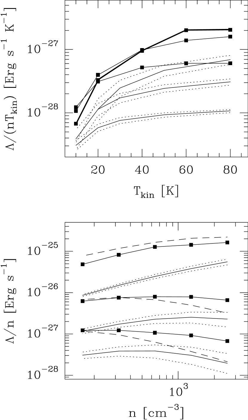
Figure 14: Cooling rate of ¹²CO averaged over the volume of the model B. In the upper panel the filled squares joined by lines are our results for cloud mean densities $<n>$=160 cm^-3 (lowest curve), 640 cm^-3 and 2560 cm^-3 (thick line). The corresponding rates computed from the formulae presented by Neufeld et al. (1995) are shown with solid lines and dotted lines correspond to column densities two times or half the estimated values of $\tilde{N}$. In the lower panel the corresponding curves are plotted as the function of density for temperatures 10, 20 and 80 K. The dashed lines are Neufeld et al. predictions for density 3$<n>$.

Figure 15: Comparison of the cooling rates $\Lambda$ computed from the analytical representation given by Neufeld et al. (1995; dotted lines) and the rates in our model $A$ (solid curve). The curves correspond to density $n\sim 10^{3}$ cm^-3. The solid curve is computed from the analytical fit of Equation 4 and is drawn only for the actual column density interval present in the model.

Neufeld et al. (1995) give cooling rate as a function of column density measure, $\tilde{N}=Gn/|dv/dx|$, i.e. number density divided by the velocity gradient or, in the absence of a gradient, by the velocity dispersion divided by distance. This is essentially the number of hydrogen atoms per velocity unit, in units of cm^-2 km^-1 s. There is, however, an additional factor, $G$, which depends on the geometry. For plane parallel medium with large velocity gradient the value is $G=1$ and in the centre of a static sphere $G\sim 0.5$. The effect of the abundance is included in the parameter $\tilde{N}$ and its value need not be known separately.

In the upper panel of Figure 14 we plot the average ¹²CO rate for model $B$, with the mean density scaled to 160, 640, and 2560 cm^-3. The parameter $\tilde{N}$ was estimated as $G\,n\,L/\sigma$ with $G=1$ and $\sigma$ equal to the rms velocity dispersion in the MHD model at given temperature. The lower three lines show predictions by Neufeld et al. (1995) and the dotted lines show the rates with $\tilde{N}$ multiplied by two or by one half. The lower panel shows the corresponding rates as function of the mean cloud density. The main difference is again due to the density inhomogeneity of MHD models. Gas with density above the average value provides most of the cooling power and the cooling rate is comparable to that of a much denser homogeneous cloud. In the low density models the Neufeld et al. formula would give a fairly good prediction of the cooling rate if density value $n\sim 3<n>$ were used. On the other hand, rate could be raised only slightly by lowering $\tilde{N}$.

Next we will discuss again the local cooling rates. In Figure 15 our ¹²CO cooling efficiencies, $\Lambda$, are shown together with the results of Neufeld et al. (1995, Table 3) as a function of $\tilde{N}$. Our curves correspond to the analytic approximation of the local cooling rate in model $B$ (see Sect. 5.2). For the plot we must determine a relation between our parameter $N_{\rm eff}$, which is a quantity integrated over the local absorption profile, and $\tilde{N}$ used by Neufeld et al. For gaussian lines we have relation $N_{\rm eff}\approx$0.3 $N/\sigma$ (see Section 5.1) while for plane-parallel flow (geometrical factor $G=1$) $\tilde{N}=N/\sigma$. This gives a conversion $N_{\rm eff}\sim 0.3\tilde{N}$ and this relation is used to plot our results on the $\tilde{N}$ scale in Figure 15. The scaling between $\tilde{N}$ and $N_{\rm eff}$ is only approximate and depends on the LVG model assumed. The curves may therefore be shifted in the horizontal direction. However, the shift should correspond to no more than a factor of two change in $\tilde{N}$.

The most important difference is the marked flattening of the column density dependence that is seen in our models at higher kinetic temperatures. This is the same effect as seen e.g. in Figures 12 and 13 and we interpret this as the consequence of varying excitation conditions that allow efficient cooling even in the dense gas. Low density gas radiates in low transitions while cooling in dense cores takes place mainly through higher transitions. At higher kinetic temperatures more transitions can contribute to the cooling and there is a clear difference between subthermally excited low density gas and cores that are close to thermalization. Different parts of the cloud are therefore decoupled not only due to velocity differences but also because they radiate mostly in different transitions. The difference between our results and those in Neufeld et al. (1995) decreases with decreasing temperature, i.e., at low kinetic temperatures our models behave more like homogeneous clouds. At low temperatures the number of excited levels is small and the remaining transitions have higher optical depth. In Figure 15 we show curves only for density $n\sim$10³ cm^-3 but the results are qualitatively similar even at other densities.

The detected differences between inhomogeneous and homogeneous cloud models can be attributed to two effects. Firstly, density and velocity inhomogeneities increase the photon escape probability. Both the excitation and the escape probability of photons are determined by the optical depths towards different lines of sight. In the center of a homogeneous cloud the optical depth is the same towards all directions. An inhomogeneous cloud with the same average optical depth has always a higher escape probability, since the escape probability is proportional to the average of exp(-$\tau$) and not to the average of $\tau$. This leads to higher escape probability but generally also to lower excitation. Secondly, in the considered models $\Lambda/n$ is still an increasing function of density and therefore density variations tend to increase the total cooling power. The slope of $\Lambda/n$ is, of course, determined by the radiative transfer and the two effects are closely interrelated. The density distribution was seen to affect the photon escape probability also indirectly through excitation. Some excitation levels are populated only in the densest regions and this leads to a partial decoupling between the dense cores and the surrounding low density gas.

7 Summary and conclusions

We have studied the radiative cooling of molecular gas at temperatures $T_{\rm kin}$=10-80 K and densities $n\lesssim 10^{4}$ cm^-3, based on three-dimensional MHD calculations of the density and velocity structure of interstellar clouds. The models have been scaled to linear sizes $\sim$6 pc and mean densities in the range 160–2560 cm^-3. The cooling rates for isothermal clouds were computed by solving the radiative transfer problem with Monte Carlo methods.

We find that:

• Inhomogeneous density and velocity fields reduce photon trapping and thus increase the cooling rates. In comparison with homogeneous cloud models the MHD models are much less affected by optical depths effects. This is especially true at kinetic temperatures $T_{\rm kin}\gtrsim$60 K.

• There is a clear difference between the density dependence of local cooling rates and the density dependence of cooling rates averaged over entire clouds.

• At low to intermediate densities most of the cooling power is provided by clumps with densities above the average gas density. The average cooling rate for a model with given mean density can be as much as an order of magnitude larger than the local cooling rate at the same density. In models with higher average density and lower temperature the differences are smaller since the densest parts of clouds become optically thick.

• Compared with earlier models (Goldsmith & Langer (1978); Neufeld et al. (1995)) our local cooling rates differ mainly at large densities where our rates are higher due to reduced photon trapping. The volume averaged cooling rates are higher than in the earlier models typically by a factor of few. At higher temperatures ($T\gtrsim 40$ K) the difference can be almost one order of magnitude.

• For the MHD models, the absence of the macroscopic velocity field would reduce the cooling by up to 10%.

• The absence of density fluctuations would reduce cooling by $\sim$50% at 10 K. This is caused mainly by the density dependence of the cooling rates and the radiative transfer effects are less important. At high temperatures ($\gtrsim$80 K) the difference to homogeneous models approaches a factor of ten.

• ¹²CO is clearly the most important coolant over the whole parameter range studied.

• At low temperatures ¹³CO is the the second most important coolant, after ¹²CO. At temperatures $T_{\rm kin}>$60 K it is exceeded by OI, which can provide more than 10% of the total cooling (assuming a relative abundance $\sim$10^-5).

• In view of the recently observed very low O₂ and H₂O abundances these species are unimportant for the cooling of the type of clouds studied in this paper.

References

- Ashby et al. (2000) Ashby M.L.N., Bergin E.A., Plume R., et al. 2000, ApJ 539, 119
- Bergin et al. (2000) Bergin E.A., Melnick G.J., Stauffer J.R. et al. 2000, ApJ 539, L129
- Bergman (1995) Bergman P. 1995, ApJ 445, L167
- Boissé (1990) Boissé P. 1990, A&A 228, 483
- Caux et al. (1999) Caux, E., Ceccarelli, C., Castets, A., et al. 1999, A&A 347, L1
- de Jong (1977) de Jong T. 1977, A&A 55, 137
- Flower & Launay (1985) Flower D.R., Launay J.M. 1985, MNRAS 214, 271
- Goldreich & Kwan (1974) Goldreich P., Kwan J. 1974, ApJ 189, 441
- Goldsmith & Langer (1978) Goldsmith P.F., Langer W.D. 1978, ApJ 222, 881
- Goldsmith et al. (2000) Goldsmith P. F., et al. 2000, ApJ 539, L123
- Harjunpää & Mattila (1996) Harjunpää P., Mattila K. 1996, A&A 305, 920
- Hartstein & Liseau (1998) Hartstein D., Liseau R. 1998, A&A, 332, 702
- Jacquet et al (1992) Jacquet R., Staemmler V., Smith M.D., Flower D.R. 1992, J.Phys.B 25, 285
- Jimenez et al. (2000) Jimenez R., Padoan P., Dunlop J., Bowen D., Juvela M., Matteucci F. 2000, ApJ 532, 152
- Juvela (1997) Juvela M. 1997, A&A 322, 943-961
- Juvela (1998) Juvela M. 1998, A&A 329, 659-682
- Juvela & Padoan (1999) Juvela M., Padoan P. 1999, in Science with the Atacama Large Millimeter Array, Wootten A. (ed), in press (astro-ph/9912154)
- Larson (1981) Larson R.B. 1981, MNRAS 194, 809
- Launay & Roueff (1977) Launay J.M., Roueff E. 1977, A&A 56, 289
- Lee et al. (1997) Lee H.-H., Bettens R.P.A., Herbst E. 1996, A&AS 119, 111
- Millar et al. (1997) Millar T.J., Farquhar P.R.A., Willacy K. 1997, A&AS 121, 139
- Neufeld & Kaufman (1993) Neufeld D.A., Kaufman M.J. 1993, ApJ 418, 263
- Neufeld et al. (1995) Neufeld D.A., Lepp S., Melnick G.J. 1995, ApJS 100, 132
- Ohishi et al. (1992) Ohishi M., Irvine W.M., Kaifu N. 1992, in Astrochemistry of Cosmic Phenomena, Singh P.D. (ed.) Kluwer Academic Publishers, Dordrecht, p. 171
- Padoan et al. (1999) Padoan P., Bally J., Billawala Y., Juvela M., Nordlund Å1999, ApJ 525, 318
- Padoan & Nordlund (1999) Padoan, P., Nordlund, Å. 1999, ApJ, 526, 279
- Padoan et al. (1998) Padoan P., Juvela M., Bally J., Nordlund Å. 1998, ApJ 504, 300
- Padoan et al. (2000a) Padoan P., Juvela M., Bally J., Nordlund Å. 2000a, ApJ 529, 259
- Padoan et al. (2000b) Padoan, P., Zweibel, E., Nordlund, Å. 2000b, ApJ, 540, 332
- Schröder et al. (1991) Schröder K., Staemmler V., Smith M.D., Flower D.R., Jacquet R. 1991, J.Phys.B 24, 2487
- Snell et al. (2000a) Snell R.L., Howe J.E., Ashby M.L.N et al. 2000a, ApJ 539, L93
- Snell et al. (2000b) Snell R.L., Howe J.E., Ashby M.L.N et al. 2000b, ApJ 539, L97
- Snell et al. (2000c) Snell R.L., Howe J.E., Ashby M.L.N et al. 2000c, ApJ 539, L101
- Spaans (1996) Spaans M. 1996, A&A 307, 271
- Warin et al. (1996) Warin S., Benayoun J.J., Viala Y.P. 1996, A&A 308, 535