Space Debris Hazards from Explosions in the collinear Sun-Earth Lagrange points

Abstract

The collinear Lagrange points of the Sun-Earth system provide an ideal environment for highly sensitive space science missions. Consequently many new missions are planed by ESA and NASA that require satellites close to these points. For example, the SOHO spacecraft built by ESA is already installed in the first collinear Lagrange point. Neither uncontrolled spacecraft nor escape motors will stay close to the Lagrange points for a long time. In case an operational satellite explodes, the fragmentation process will take place close to the Lagrange point. Apparently a number of spacecraft will accumulate close to the Lagrange points over the next decades. We investigate the space debris hazard posed by these spacecraft if they explode and fall back to an Earth orbit. From our simulation we find that, as expected, about half of the fragments drift towards the Earth while the other half drifts away from it. Around $2\%$ of the simulated fragments even impact the Earth within one year after the explosion.

1 Introduction

The hazards to manned as well as unmanned satellites by breakups of satellites and rocket upper stages in low Earth orbit (LEO) and geo-stationary orbit (GEO) have been extensively discussed in the literature [1990, 1993, 1993, 1995, 1997, 1997]. Since the early 1970ies [1973] there are considerations to use another class of orbits: quasi-stable trajectories around the Lagrange points of the Sun-Earth system. Especially the collinear points ${\rm L}_{1}$ and ${\rm L}_{2}$ (see figure 1) are interesting for solar physics and space science applications [1998]. Since orbits around the collinear libration points are inherently instable, the dwell time of rocket bodies or uncontrolled satellites is short and thus breakups of these objects are less likely than in LEO or GEO. Breakups of malfunctioning operational satellites, however, create a cloud of fragments on the stable manifold. The stable manifold connects the locations of periodic motion in the six-dimensional phase space of the satellite [1980].

Figure 1: Illustration of the position of the Lagrangian points of equilibrium in the Sun-Earth system. The Sun is at the centre of the plane representing the orbital plane of the Earth, and the horizontal axis is fixed to the Sun-Earth line.

In order to model the fragmentation process, we apply a fragmentation model that combines the fragment mass distribution by Bess [1975] with the $\Delta v$ distribution taken from the explosion model by Reynolds [1990]. From these models, the differential fragment mass distribution of a low intensity explosion is given by (see also Jehn [1990]):

$$nd\!m = \left\{\begin{array}[]{l}1.71\times 10^{-4}M_{t}\exp(-0.02056\sqrt{m})\\ \mbox{\hskip 14.22636ptfor }m>1936\>{\rm g}\\ 8.69\times 10^{-4}M_{t}\exp(-0.05756\sqrt{m})\\ \mbox{\hskip 14.22636ptfor }m<1936\>{\rm g}\end{array}\right.$$ (5)

with $M_{t}$ being the total mass of the satellite. Assuming an average fragment mass density of $\rho=4.7\>{\rm g}\>{\rm cm}^{-3}$, the fragment diameter $d$ is given by

$$\frac{d}{2} = \sqrt[3]{\frac{3m}{4\pi\rho}}.$$ (6)

According to Reynolds, the $\Delta v$ of a fragment in $[{\rm m}\>{\rm s}^{-1}]$ is given as a function of fragment diameter $d$ in $[{\rm m}]$ :

$$\log\Delta v = -0.0676\left(\log d\right)^{2}-0.804\log d$$

$$-1.514$$

We simulate an explosion close to ${\rm L}_{2}$ using the models described above. A total number of $820$ fragments is generated, that drift off the point of equilibrium depending on the direction and the magnitude of the $\Delta v$ imposed on the fragment by the explosion. Figure 2 shows the distribution of $\Delta v$ in the simulated fragment cloud. We assume that the fragments are distributed isotropically. After the simulated breakup we propagate the fragments for one year, taking into account the gravity of the Earth, the Sun, the Moon, as well as the oblateness of the Earth and solar radiation pressure. In the following sections we describe the motion of the simulated fragments, as well as the potential threat they pose to operational satellites.

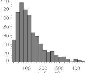
Figure 2: Histogram of the distribution of $\Delta v$ of the generated fragments (total number: $820$).

2 Motion of the Fragments

The dynamics of the fragments is dominated by the effective potential in the Earth-fixed frame of the restricted three-body problem. Thus, the fragment motion depends on the Jacobian constant that is determined by the breakup process. Before the breakup, the satellite is assumed to have the Jacobi constant of the ${\rm L}_{2}$ point of $C_{0}=-3.0008926$ in canonical units (distance unit $=1\>{\rm AU}$, mass unit $=M_{\odot}+M_{\oplus}$, time unit such that period of Earth’s orbit equals $2\pi$). For this value of $C$, the satellite is at the intersection of zero-velocity curves (ZVC), i.e., in equilibrium motion. Since the satellite is in rest with respect to the Earth-fixed frame, the breakup always increases the value of $C$. Because we consider lunar gravity, the Earth’s oblateness, and radiation pressure, the Jacobi “constant” is not exactly constant along the fragment’s trajectories. The value of $C$ can be decreased by lunar perturbations (e.g. by close fly-bys), or by the effect of the Earth’s oblateness during close Earth encounters. Figure 3 shows the distribution of $C$ for all $820$ fragments $30\>{\rm days}$ after the breakup.

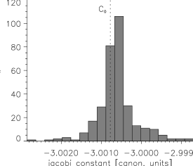
Figure 3: Histogram of the distribution of the Jacobi constant of the generated fragments (total number: $820$). The dotted line indicates the initial value of the constant before the breakup.

Figure 4: Zero velocity curves (ZVCs) in the Earth-fixed system for different values of the Jacobi constant. A plane $0.1\times 0.1\>{\rm AU}$ around the Earth is shown, the Sun (not on the diagram) is at the origin. The contour lines (solid for $C>C_{0}$, dashed for $C=C_{0}$, dotted for $C<C_{0}$) represent ZVCs for $C=C_{0},C_{0}\pm 0.001,C_{0}\pm 0.0005,andC_{0}\pm 0.0001$.

Figure 5: Trajectories (solid lines) of an explosion fragments in the Earth’s orbital plane. In panel (a) a region $11\times 11\>{\rm AU}$, and in panels (b)-(d) a region $4\times 4\>{\rm AU}$ are shown with the Earth at the origin. The dotted circle indicates the orbit of the Moon and the dashed line the Sun-Earth line. The Sun is located at $149\times 10^{6}\>{\rm km}$ along the positive $x$-axis. The cross-markers along the trajectories indicate the fragment’s position separated by $20\>{\rm days}$. Panel (a) shows an Out-bound directed trajectory, panel (b) a typical in-bound trajectory, and panels (c) and (d) in-bound trajectories that are captured into bound orbits around the Earth.

The breakup creates a rather narrow distribution of the Jacobian constant around the equilibrium value $C_{0}$. Fragments with $C<C_{0}$ are confined either to a region close to the Earth or to outside a ring around the Earth’s orbit. This restriction can be seen in figure 4 that shows the ZVCs for fragments with different values of $C$. For $C>C_{0}$ the fragments may move freely along the Sun-Earth line, but not along the Earth’s orbit. In general two classes of orbits are possible: out-bound and in-bound. Fragments on out-bound orbits move away from the Earth so that they have larger heliocentric semi-major axes and smaller mean motions. Consequently they drift into the positive $y$-direction, which is opposite to the direction of motion of the Earth around the Sun (see figure 5 (a)). These fragments, which constitute $44\%$ of the simulated objects, continue on independent heliocentric orbits and therefore pose no threat to Earth satellites. The other class of orbits are in-bound to the Earth that potentially exhibit close lunar or Earth encounters. If no close encounters occur, the orbits around the Earth are very unstable, as shown in figure 5 (b). Mostly lunar fly-bys decrease the orbital energy (and thus the value of $C$) of some fragments, so that they stay in bound orbits about the Earth for more than one year (see figures 5 (c) and (d)).

3 Potential Hazards to Operational Satellites

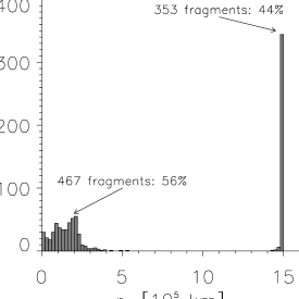
Figure 6: Histogram of the perigee distribution of the fragments (total number: 820) one year after the breakup.

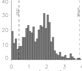
Figure 7: Zoom of the perigee range from $0$ to $4\times 10^{5}\>{\rm km}$ in figure 6. The dashed lines indicate the distance range of the GEO ring and the lunar orbit.

In our simulation $56\%$ of the fragments moved towards the Earth along the Sun-Earth line. Whether or not they pose a threat to operational satellites depends on whether they reach LEO or GEO distances, i.e. on their perigee distance $r_{\pi}$. Figure 6 shows the distribution of $r_{\pi}$ for all $820$ fragments, propagated over one year. The peak at $1.5\times 10^{6}\>{\rm km}$ indicates the $353$ ($44\%$) fragments on out-bound orbits that never approach the Earth closer than the distance of ${\rm L}_{2}$. The $467$ ($56\%$) fragments on in-bound orbits almost always approach the Earth closer than the lunar orbit. Figure 7 shows a zoom of the fragment perigee distribution inside the lunar orbit. The maximum of the perigee distribution is at $2\times 10^{5}\>{\rm km}$, far outside the orbit of most operational satellites. While less than $60$ fragments approached the Earth closer than GEO, no fragment actually intersected the GEO ring. In addition, a crossing of fragments from ${\rm L}_{2}$ of the GEO ring is only possible around the equinoxes when the GEO ring intersects the Sun-Earth line.

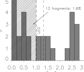
Figure 8: Zoom of the perigee range from $0$ to $3R_{\oplus}$ (Earth radii) in figure 7. The dashed lines indicate the boundaries of the LEO region and the hashed area indicates the extend of the Earth.

Due to their low initial angular momentum (or transversal velocity) with respect to the Earth, fragments can actually impact the Earth’s surface. In our simulation $17$ fragments reached the LEO environment ($H<2000\>{\rm km}$), and $13$ ($1.6\%$) impacted the Earth close to Earth escape velocity (see figure 8). Despite the fact that the out-of plane motion of the fragments stays small, they can impact the Earth at any latitude, because the Earth’s diameter small is compared to the distance to ${\rm L}_{2}$(see figure 9).

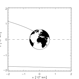
Figure 9: Trajectory (solid line) of an impacting fragment in the Earth’s vicinity. The $x$-direction is the Sun-Earth line and the $z$-direction is perpendicular to the Earth’s orbital plane. At the bottom a segment of the fragment’s trajectory from an earlier close encounter can be seen. The final segment of the trajectory approaches the Earth from the upper left corner.

4 Conclusion

The use of the collinear Sun-Earth Lagrange points for solar physics and space science application is expected to increase. Therefore, a breakup of a controlled satellite due to a malfunction can not be ruled out. Since the dwell time of uncontrolled satellites and rocket bodies close to the libration points is short, they are unlikely to contribute to the hazard to operational satellites due to breakups at these points. If an explosion of a satellite occurs close to ${\rm L}_{2}$, about $50\%$ of the fragments move in-bound towards the Earth. Collisions of the fragments with GEO satellites are very unlikely and are possible only if the breakup occurs close to the vernal or autumnal equinox. A low percentage (about $2\%$) of the fragments reaches the LEO environment and impacts the Earth’s atmosphere with velocities close to the Earth’s escape speed of $11\>{\rm km}\>{\rm s}^{-1}$. These Earth impacts can happen at any geographic latitude and longitude.

References

- 1975 Bess, T. D. 1975. Size Distribution of Fragment Debris Produced by Simulated Meteoroid Impact of Spacecraft Wall. TN D-8108. NASA/Langley Research Center.
- 1973 Farquhar, R. W. 1973. Quasi-Periodic Orbits about the Translunar Libration Points. Celestial Mechanics, 7, 458–473.
- 1998 Farquhar, R. W. 1998. The Flight of ISEE-3/ICE: Origins, Mission History, and a Legacy. AIAA 98-4464.
- 1993 Fucke, W. 1993. Fragmentation Experiments for the Evaluation of the Small Size Debris Population. Pages 275–280 of: Flury, W. (ed), Proceedings of the First European Conference on Space Debris. Darmstadt, Germany: Mission Analysis Section, ESOC, for ESA.
- 1997 Houchin, P. P., Crowther, R., & Walker, R. J. 1997. Analysis of a Break-Up Event in Orbit. Pages 293–297 of: Kaldeich-Schürmann, B., & Harris, B. (eds), Proceedings of the Second European Conference on Space Debris. ESTEC, Noordwijk, The Netherlands: ESA Publications Division, for ESA.
- 1990 Jehn, R. 1990. Fragmentation Models. Working Paper 312. ESA/MAS.
- 1995 Jehn, R. 1995. Modelling Debris Clouds. Ph.D. thesis, Technische Hochschule Darmstadt.
- 1997 Matney, M., & Settecerri, T. 1997. Characterization of the Breakup of the Pegasus Rocket Body 1994-029B. Pages 289–292 of: Kaldeich-Schürmann, B., & Harris, B. (eds), Proceedings of the Second European Conference on Space Debris. ESTEC, Noordwijk, The Netherlands: ESA Publications Division, for ESA.
- 1993 McKnight, D. S., & Nagl, L. 1993. Key Aspects of Satellite Breakup Modeling. Pages 269–274 of: Flury, W. (ed), Proceedings of the First European Conference on Space Debris. Darmstadt, Germany: Mission Analysis Section, ESOC, for ESA.
- 1990 Reynolds, R. C. 1990. A Review of Orbital Debris Environment Modeling at NASA/JSC. AIAA-90-1355.
- 1980 Richardson, D. 1980. Periodic Orbits About the Collinear Points. Celestial Mechanics, 22, 241–253.