[

Tests for Gaussianity of the MAXIMA-1 CMB Map

Abstract

Gaussianity of the cosmological perturbations in the universe is one of the key predictions of standard inflation, but it is violated by other models of structure formation such as topological defects. We present the first test of the Gaussianity of the cosmic microwave background (CMB) on sub-degree angular scales, where deviations from Gaussianity are most likely to occur. We apply the methods of moments, cumulants, the Kolmogorov test, the $\chi^{2}$ test, and Minkowski functionals in eigen, real, Wiener-filtered and signal-whitened spaces, to the MAXIMA-1 CMB anisotropy data. We conclude that the data, which probe angular scales between 10 arcminutes and 5 degrees, are consistent with Gaussianity.

]

A. Introduction: The anisotropy in the cosmic microwave background (CMB) is arguably the cleanest cosmic signal that preserves the intrinsic statistical properties of cosmological perturbations [1]. The recent observations from MAXIMA-1 [2] and BOOMERANG [3] have unambiguously detected a sharp peak in the CMB power spectrum. This has favored inflation [4] as the dominant mechanism for structure formation of the universe [5] as opposed to other candidates like topological defects [6]. Another key prediction of standard inflation is that the distribution of cosmic perturbations are Gaussian, while other cosmological models such as isocurvature inflation (e.g. [7]) and topological defects (e.g. [8]) predict otherwise. Thus tests for the Gaussianity of CMB anisotropy data can discriminate between cosmological models. In addition, a Gaussian distribution is an important ingredient in the estimation algorithm of CMB power spectra [9, 10], which has been used to produce the recent MAXIMA-1 and BOOMERANG results [2, 3]. Adding the fact that the estimation of cosmological parameters [11, 12, 13] relies on the estimated CMB power spectra, it is important to verify the Gaussian distribution of the CMB.

Tests for the Gaussianity of CMB data have been carried out by numerous authors, mainly using data from the Differential Microwave Radiometer (DMR) on the COsmic Background Explorer (COBE) [14]. Several statistics were used including moments, cumulants, Minkowski functionals (which include genus, e.g. [15, 16]), the three-point function (e.g. [17]), bispectrum (e.g. [18, 19]), wavelet transform (e.g. [20]), etc. All these tests showed that the data were consistent with Gaussianity, except for a couple of results [19, 20] that may have non-cosmological origins [21].

In addition to the usual limitations from foreground contamination and instrumental noise, the $7^{\circ}$ angular resolution of the DMR data is not ideal for tests of Gaussianity. Angular resolution is an issue because the size of the causal horizon at last scattering is about one degree. Thus in a sky patch of super-degree size, there are many uncorrelated perturbations due to causality. As a result, the central limit theorem guarantees that the pre-last-scattering anisotropy on super-degree scales will tend to be Gaussian. Even if the post-last-scattering anisotropy is strong and non-Gaussian, it can be obscured by the pre-last-scattering contribution, which we expect to be Gaussian. Therefore a CMB map with sub-degree resolution can provide much more powerful tests for Gaussianity. Park et al. [22] recently used a genus test on the QMAP and Saskatoon data, which have a resolution of about $1.5^{\circ}$, to show that they were consistent with Gaussianity. In this paper we report results from a series of Gaussianity tests on the MAXIMA-1 CMB map [2], which provides anisotropy information on angular scales between $10^{\prime}$ and $5^{\circ}$. To optimize both the resolution and the signal-to-noise ratio for these tests, we shall use a map with 5972 square pixels of $8^{\prime}$ each [23]. Using these high-quality data we probe for the first time the Gaussianity of CMB anisotropy on sub-degree scales.

A CMB sky is Gaussian if it is a realization of a process that is only specified by the two-point correlation function of a given cosmological model. However, because we have only one realization of the CMB sky, it is not possible to exhaustively test the statistical properties of the process that generated it. Therefore, we employ a Frequentist approach, testing the null hypothesis of Gaussianity for the inflationary model that best fits the data.

B. Karhunen-Loève transform: We consider the Karhunen-Loève (K-L) transform, sometimes called Principal Component Analysis or the signal-to-noise eigenmode transformation [24, 9], because it enables us not only to transform the observed CMB map into uncorrelated eigenmodes of known signal-to-noise ratios, and further to implement Gaussianity tests on the uncorrelated modes. For the CMB, it is standard to model the data ${\bf d}\equiv d_{i}$ as a linear sum of uncorrelated signal ${\bf s}\equiv s_{i}$ and noise ${\bf n}\equiv n_{i}$, with the correlation matrix ${\bf C\equiv\langle dd^{\rm T}\rangle=S+N}$ where ${\bf S=\langle ss^{\rm T}\rangle}$ and ${\bf N=\langle nn^{\rm T}\rangle}$. In the noise-whitened space ${\bf d}^{\rm(W)}={\bf N}^{-1/2}{\bf d}$, all the eigenvalues of the noise matrix, ${\bf N}^{-1/2}{\bf N}{\bf N}^{-1/2}={\bf I}$, are simply unity. Thus the eigenvalues ${\bf e}^{S({\rm W})}$ of the noise-whitened signal matrix ${\bf N}^{-1/2}{\bf S}{\bf N}^{-1/2}$ represent the square of signal-to-noise ratios of each eigenmode. The coefficients ${\bf b}^{\rm(W)}$ of the noise-whitened eigenmodes in a data set can be obtained by transforming ${\bf d}^{\rm(W)}$ to the basis which diagonalizes ${\bf N}^{-1/2}{\bf C}{\bf N}^{-1/2}$. These coefficients are normally called the K-L coefficients.

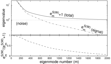
We compute ${\bf S}$ using the CMB power spectrum of the best estimated cosmological model [11] ($\Omega_{b}=0.105$, $\Omega_{c}=0.595$, $\Omega_{\Lambda}=0.3$, and $h=0.53$) and including the effects introduced by the beam shape and the pixelization of the map [25]. The matrix ${\bf N}$ is estimated from the temporal data [23]. The resulting eigenvalues in the noise-whitened space are shown in Fig. 1, sorted in descending order. The dot-dashed line indicates that only the first 639 modes have signal-to-noise ratios $\left[{\bf e}^{S({\rm W})}\right]^{1/2}\geq 1$. This number is well below our pixel number 5972. It is determined by the signal and noise levels and the observing resolution (beam) of a data set, but is independent of the pixel number of the map when the pixel size is not larger than the observing resolution.

A common technique to remove the information of non-cosmological interest in the map is Wiener filtering, ${\bf d}^{\rm WF}={\bf SC}^{-1}{\bf d}$. This is equivalent to weighting the eigenmodes with the ratios ${\bf e}^{S({\rm W})}/({\bf e}^{S({\rm W})}+1)$ (see Fig. 1). The sum of these ratios for all the eigenmodes is 837, again well below the total number 5972 of the eigenmodes. We shall employ this technique in section D to amplify the statistical significance of the CMB signal in our map.

The K-L transform can also be used to test for Gaussianity. If the underlying map is Gaussian, then the eigenvalue-normalized K-L coefficients ${\bf a}^{{\rm(W)}}\equiv{\bf b}^{{\rm(W)}}/({\bf e}^{S{\rm(W)}}+1)^{1/2}$ should be a set of Gaussian variables with mean zero and variance one. We compute the ${\bf a}^{{\rm(W)}}$ of our data, and use the observed frequency distribution to approximate its one-point probability distribution functions (PDF) $p(\nu)$, where $\nu$ is the number of standard deviations from the mean, for both the entire 5972 and the first 639 modes (i.e., those modes with signal dominating over noise). Both cases easily pass the $\chi^{2}$ and the Kolmogorov tests for Gaussianity at 95% confidence.

FIG. 1.: Noise-whitened eigenvalues of the MAXIMA-1 CMB data (top), and the Wiener filter (bottom).

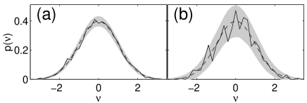
In addition to the above tests, we also use Monte Carlo (MC) simulation to build a Gaussian reference frame for the Frequentist approach. We generate 100,000 Gaussian realizations, each of which is obtained by $d^{\rm MC}_{i}=C^{1/2}_{ij}g_{j}$, where $g_{j}$ is a Gaussian variable of mean zero and variance one. As a first application, we use the MC simulation to find the probability distribution of $p(\nu)$ at each $\nu$ for the entire 5972 and the first 639 ${\bf a}^{{\rm(W)}}$. Fig. 2 shows that in both cases the real data lie well within the 95% confidence regions of Gaussianity (hereafter CRG). We also compute the moments and cumulants of the first 639 ${\bf a}^{{\rm(W)}}$ up to tenth order, and they are all well within the 99% CRG. All these results support the conclusions not only that our map is consistent with Gaussianity, but also that our estimations of noise and CMB power spectrum (giving ${\bf N}$ and ${\bf S}$ respectively) are consistent with the data so as to provide the proper eigenmodes for the K-L transform.

FIG. 2.: PDF $p(\nu)$ of the entire 5972 (a) and the first 639 (b) ${\bf a}^{{\rm(W)}}$ of the MAXIMA-1 data (solid), the Gaussian expectation (dashed), and its 95% CRG (shaded).

C. Minkowski functionals: The concept of Minkowski functionals is based on integral geometry. According to Hadwiger’s Theorem $\beta+1$ Minkowski functionals are sufficient to measure the morphology of a $\beta$-dimensional pattern. In the case of CMB we have $\beta=2$ and thus need only three Minkowski Functionals. First we define the excursion set $Q$ in a given CMB field as the region in which the CMB amplitude $d_{i}$ is larger than a threshold: $Q\equiv Q(\nu)=\{d_{i}|(d_{i}-\mu)/\sigma>\nu\}$, where $\mu=\langle d\rangle$ and $\sigma^{2}=\langle d^{2}\rangle-\mu^{2}$. Then the surface densities $v_{i}(\nu)\equiv V_{i}(Q)/A$ of Minkowski functionals $V_{i}(Q)$ for a CMB patch of angular area $A$ can be defined as

$$v_{0}=\frac{1}{A}\int_{Q}dA,\;v_{1}=\frac{1}{4A}\int_{\partial Q}dl,\;v_{2}=\frac{1}{2\pi A}\int_{\partial Q}\kappa dl,$$ (1)

where $\partial Q$ is the boundary of the region $Q$, $dA$ and $dl$ are the differential elements of $Q$ and $\partial Q$ respectively, and $\kappa$ is the geodesic curvature of $dl$. These Minkowski Functionals have different morphological meanings: $V_{0}$ is the total area of $Q$, $V_{1}$ is the total length of its boundary, and $V_{2}$ is the number of isolated regions (hot spots) in $Q$ minus the number of holes (cold spots). For an isotropic Gaussian field these functionals are characterized only by the field’s variance $\sigma^{2}$ and the variance of its gradient $\tau=\langle|{\bf\nabla}d|^{2}\rangle/2$, i.e. $v_{0\rm(G)}={\rm erfc}(\nu/\sqrt{2})/2$, $v_{1\rm(G)}=\tau^{1/2}\exp(-\nu^{2}/2)/8\sigma$, and $v_{2\rm(G)}=\tau\nu\exp(-\nu^{2}/2)/(2\pi)^{3/2}\sigma^{2}$. We also note that the commonly used one-point PDF $p(\nu)$ and genus $g$, or the ‘Euler-Poincaré characteristics’, are simply related to the Minkowski Functionals. For the two-dimensional CMB, we have $p(\nu)=-\partial V_{0}/A\partial\nu$ and $g=V_{2}+{V_{0}}/{2\pi}$.

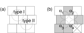
Because the MAXIMA-1 map has an irregular boundary and all pixels have a square shape lying on a regular lattice, we need a numerical scheme to approximate its Minkowski Functionals. For a given threshold $\nu$ and thus a given $Q$ on the lattice, $v_{0}$ is simply the number of pixels in $Q$ divided by the total number of pixels in the map. Here $v_{1}$ is determined by the length of $\partial Q$ multiplied by $\pi/4$ to correct for the square-pixel lattice effect. To compute $v_{2}$, we first induce offset in the pixel positions every other row. As Fig. 3 (a) shows, this gives two types (I and II) of vertices. For each type, the integration of $\kappa$ in equation (1) can be easily obtained by examining the status of the neighboring four pixels (basically the integration is determined by the change of the internal angle along $\partial Q$). Fig. 3 (b) shows an example, where the pixels in $Q$ are shaded and the one with no CMB data is labeled with a cross. In this case the vertices $\alpha_{1}$, $\alpha_{2}$, $\alpha_{3}$ and $\alpha_{4}$ have unambiguously $\int_{\alpha_{i}}(2\kappa/\pi)dl=-2$, $2$, $-1$ and $0$ respectively, while a confusion in this calculation would occur at $\alpha_{1}$and $\alpha_{2}$ if there was no offset every other row. We also notice that any bias possibly induced by the above algorithms should disappear when the number of pixels is large, as in our case.

FIG. 3.: (a) Vertices of type I and II formed by inducing an offset in the pixel positions every other row. (b) An example of a pixelized CMB map with the artificial pixel offset.

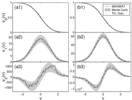
We compute the $v_{0}(\nu)$, $v_{1}(\nu)$, and $v_{2}(\nu)$ for both the entire map and the central $37\%$ (2209 pixels, covering about $6.3^{\circ}\times 6.3^{\circ}$), expected to have the lowest noise. We use pixel sizes of $8^{\prime}$, $16^{\prime}$, and $24^{\prime}$, the last two obtained by averaging the neighboring pixels of the original map. The results of all six cases lie within the $95\%$ CRG obtained from the MC simulation described earlier. Fig. 4 shows the results of the two cases with $8^{\prime}$ pixels. We note that while the means of the MC simulation (dashed lines) are close to the analytical isotropic Gaussian forms (dotted lines) in (b1–b3), they deviate significantly from each other in (a1–a3). This is due to the higher noise level near the edge of the map, contributing as an anisotropic component in the map (the RMS noise of the full map and the central part are about $162\mu K$ and $57\mu K$ respectively).

FIG. 4.: Minkowski functionals (solid) of the entire MAXIMA-1 map (a) and the central part (b). The Gaussian expectation obtained from the MC simulation (dashed), its $95\%$ CRG (shaded), and the analytic Gaussian forms (dotted).

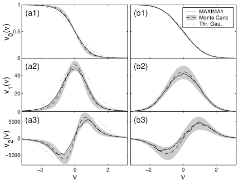
We also note that some results (solid lines) appear to have systematic departure from the Gaussian expectations $\bar{v}^{\rm MC}_{i}(\nu)$ (dashed lines). For example, (b3) shows the number of cold spots is less than the Gaussian expectation. To determine whether these discrepancies are really systematic, we first define

$$I_{i}(\nu)=\int_{-\infty}^{\nu}\frac{v_{i}(\nu^{\prime})-\bar{v}^{\rm MC}_{i}(\nu^{\prime})}{\sigma^{\rm MC}_{i}(\nu^{\prime})}d\nu^{\prime},\quad i=0,1,2,$$ (2)

where $\sigma^{\rm MC}_{i}(\nu^{\prime})$ is the standard deviation of $v_{i}(\nu^{\prime})$ estimated from the MC simulation. Applying this to both the real data and the MC simulation, we obtain respectively the $\hat{I}_{i}(\nu)$ and its Gaussian-expected PDF $p(I_{i}(\nu))$. The results from all six cases lie well within the 95% CRG. Thus we know that the apparent systematic deviations from Gaussianity in $v_{i}$ are statistically insignificant as measured by $I_{i}(\nu)$.

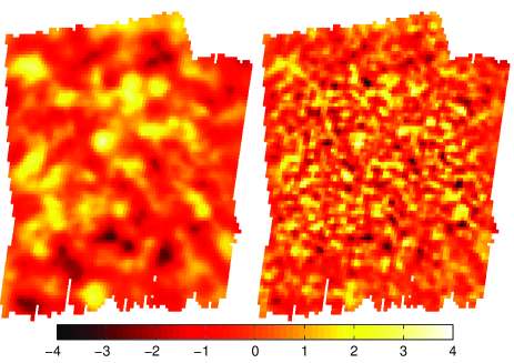
D. Wiener filtering and signal-whitening techniques: To increase the statistical significance of the CMB signal in the map, we now consider two filtering methods. One is the Wiener filtering addressed earlier, and the other is a new signal-whitening technique ${\bf d}^{\rm W}={\bf S}^{1/2}{\bf C}^{-1}{\bf d}$ [26], which not only removes the anisotropy on scales where the noise dominates (as in Wiener filtering) but also equalizes the anisotropy amplitudes on scales where the CMB signal dominates. The signal-whitening procedure will reveal in ${\bf d}^{\rm W}$ the features of the non-Gaussian components whose contribution in the CMB anisotropy dominates the Gaussian one within at least a range of the accessible scales [26]. We apply these filtering methods to both the real map (Fig. 5) and the MC simulation, and then compute their Minkowski functionals. We find that for both the entire map and the central part (as previously) the $v_{i}(\nu)$ and $I_{i}(\nu)$ of the filtered maps are within the 95% CRG. Fig. 6 shows results of the filtered central maps. We also verify for both of the filtered maps that none of the pixels with amplitude outside the $\pm 2\sigma$ range coincides with the locations of any known radio or IRAS point sources [27]. Thus we have no statistically significant detection of localized non-Gaussianity in our data.

FIG. 5.: The Wiener-filtered (left) and the signal-whitened (right) MAXIMA-1 map, with ranges of fluctuations of $(-3.1,3.4)\sigma$ and $(-3.7,4.3)\sigma$ respectively.

FIG. 6.: Similar to Fig. 4, but for the Wiener filtered (a) and the signal-whitened (b) MAXIMA-1 central map.

E. Conclusion: We employ moments, cumulants, the Kolmogorov test, the $\chi^{2}$ test, and Minkowski functionals in eigen, real, Wiener-filtered and signal-whitened spaces to implement a total of 82 (not independent) hypothesis tests for Gaussianity (22 in Sec. B, 36 in Sec. C, 24 in Sec. D), and show that the MAXIMA-1 CMB map is consistent with Gaussianity on angular scales between $10^{\prime}$ and $5^{\circ}$. This gives us confidence in the Gaussian distribution used in our estimation of the CMB angular power spectrum [2], and consequently in the estimation of cosmological parameters [11, 13]. Although our results are consistent with standard inflation and the CMB power spectrum of recent observations has favored inflation as the dominant mechanism for structure formation [5], the existence of topological defects is still possible. More sophisticated methods or data with even higher resolution and signal to noise ratio will be required to fully explore this possibility.

Acknowledgments—JHPW and AHJ acknowledge support from NASA LTSA Grant no. NAG5-6552 and NSF KDI Grant no. 9872979. PGF acknowledges support from the Royal Society. RS and SH acknowledge support from NASA Grant NAG5-3941. BR and CDW acknowledge support from NASA GSRP Grants no. S00-GSRP-032 and S00-GSRP-031. MAXIMA is supported by NASA Grant NAG5-4454 and by the NSF through the Center for Particle Astrophysics at UC Berkeley, NSF cooperative agreement AST-9120005.

REFERENCES

- [1] For a review see W. Hu, N. Sugiyama & J. Silk, Nature386, 37 (1997)
- [2] S. Hanany et al., ApJ545, L5 (2000)
- [3] P. de Bernardis et al., Nature404, 955 (2000)
- [4] A. H. Guth, Phys. Rev. D23, 347 (1981)
- [5] F. R. Bouchet et al., astro-ph/0005022 (2000); U.-L. Pen, U. Seljak & N. Turok, Phys. Rev. Lett.79, 1611 (1997)
- [6] For a review see A. Vilenkin & E. P. S. Shellard, ‘Cosmic strings and other topological defects’, Cambridge University Press, Cambridge (1994)
- [7] P. J. E. Peebles, ApJ510, 523 (1999); P. J. E. Peebles, ApJ510, 531 (1999).
- [8] P. P. Avelino, E. P. S. Shellard, J. H. P. Wu & B. Allen, ApJ507, L101 (1998).
- [9] J. R. Bond, A. H. Jaffe & L. E. Knox, Phys. Rev. D57, 2117 (1998)
- [10] J. Borrill, in Proceedings of the 5th European SGI/Cray MPP Workshop, ‘MADCAP: The Microwave Anisotropy Dataset Computational Analysis Package’ (1999; astro-ph/9911389)
- [11] A. Balbi et al., ApJ545, L1 (2000)
- [12] A. E. Lange et al., Phys. Rev. D63, 42001 (2001)
- [13] A. H. Jaffe et al, Phys. Rev. Lett.86, 3475 (2001)
- [14] G. F. Smoot et al., ApJ396, L1 (1992)
- [15] H. Minkowski, Mathematische Annalen 57, 447 (1903); J. Schmalzing & K. M. Górski, Mon. Not. R. Astron. Soc. 297, 355 (1998)
- [16] G. F. Smoot et al., ApJ437, 1 (1994); A. Kogut et al., ApJ464, L29 (1996)
- [17] X. Luo, Phys. Rev. D49, 3810 (1994); G. Hinshaw et al., ApJ446, L7 (1995)
- [18] A. F. Heavens, Mon. Not. R. Astron. Soc. 299, 805 (1998)
- [19] P. G. Ferreira, J. Magueijo & K. M. Gorski, ApJ503, L1 (1998)
- [20] J. Pando, D. Valls-Gabaud & L.-Z. Fang, Phys. Rev. Lett.81, 4568 (1998)
- [21] A. J. Banday, S. Zaroubi & K. M. Gorski, ApJ533, 575 (2000); B. C. Bromley & M. Tegmark, ApJ524, L79 (1999)
- [22] C.-G. Park et al., astro-ph/0102406 (2001)
- [23] R. Stompor et al., in preparation.
- [24] C. W. Therrien, ‘Discrete Random Signals and Statistical Signal Processing’, (Englewood Cliffs: Prentice-Hall), 1992; J. R. Bond, Astrophys. Lett. Comm. 32, 63 (1995); J. R. Bond, Phys. Rev. Lett.74, 4369 (1995); M. Tegmark, A. Taylor & A. Heavens, ApJ480, 22 (1997); E. F. Bunn & M. White, ApJ480, 6 (1997)
- [25] J. H. P. Wu et al., ApJS. 132, 1 (2001)
- [26] J. H. P. Wu, astro-ph/0012206 (2000)
- [27] We thank R. Paladini for providing us with the data.