An efficient parallel tree-code for the simulation
of self-gravitating systems

We describe a parallel version of our tree-code for the simulation of self-gravitating systems in Astrophysics. It is based on a dynamic and adaptive method for the domain decomposition, which exploits the hierarchical data arrangement used by the tree-code. It shows low computational costs for the parallelization overhead – less than 4% of the total CPU-time in the tests done – because the domain decomposition is performed ‘on the fly’ during the tree setting and the portion of the tree that is local to each processor ‘enriches’ itself of remote data only when they are actually needed. The performances of an implementation of the parallel code on a Cray T3E are presented and discussed. They exhibit a very good behaviour of the speedup ($=15$ with $16$ processors and $10^{5}$ particles) and a rather low load unbalancing ($<10$% using up to 16 processors), achieving a high computation speed in the forces evaluation ($>10^{4}$ particles/sec with 8 processors).

1 Introduction

Tree-codes (Barnes & Hut BH (1986), hereafter BH; Hernquist H (1987)) are particle algorithms extensively employed in the simulations of large self-gravitating astrophysical systems. They have the capability to speed up the numerical evaluation of the gravitational interactions among the $N$ bodies of the system. Of course, the parallelization of the algorithm aims at attaining larger and larger $N$ in the numerical representation of the real system; this is important not only to improve the spatial resolution, but also to get much more meaningful results, because a too low number of ‘virtual’ particles in comparison with the number of real bodies, gives rise to a unphysical shortening of the 2-body collisions time.

In general, an efficient parallelization means a data distribution to the processors, the so called domain decomposition (DD), so as to i) distribute the numerical work as uniformly as possible, ii) minimize the data exchange among the processors (hereafter PEs). Of course, this latter point is relevant only on distributed memory platform. Moreover, such DD should be performed with a minimal computational cost.

In the numerical evaluation of the gravitational interactions it is difficult to deal with these tasks, because the long-range nature of gravity makes data transfer among PEs unavoidable. Furthermore, self-gravitating systems have often non-uniform mass distributions, that give rise to very inhomogeneous distributions of the work-load (the amount of calculations needed to evaluate the acceleration of a particle). This implies that the DD should be weighted, in some way, according to the work-load.

Finally, the hierarchical arrangement of the subsets of the mass distribution which the tree-code is based on, implies that most of the computations for evaluating the acceleration of a particle regard the evaluation of the force due to close bodies. This suggests a spatial DD: each domain should be enclosed in a volume as contiguous and compact as possible.

At present, one of the most used approach for the DD is the orthogonal recursive bisection (Warren & Salmon orb (1992); Dubinski dubinsky (1996); Lia & Carraro carraro (2000); Springel et al. gadget (2000)), which consists in a recursive subdivision of the space in pairs of sub-domains equally weighted. On every sub-domain, the owning PE builds (independently of the others) its local tree data structure. Such structure is then enlarged enclosing those data, belonging to remote trees, that are needed to the local forces evaluation.

The main disadvantage of this approach is that the retrieval of remote data is complicated (and computationally expensive, too) mainly because of the lack of an addressing reference scheme common to all the PEs. The ‘hashed oct-tree’ method (Warren & Salmon hashed (1993), hereafter WS) solves this problem, but a certain implementation complexity still remains and some radical changes are required in the way the tree arrangement is usually stored. For this reason we decided to carry out a new and easy to implement method for sharing efficiently the computational domain among PEs in a distributed memory architecture.

This paper is organized as follows. In Sect. 2 we describe the differences of our tree-code in respect with the original method illustrated in BH, both from the general point of view of the algorithm and in connection with the parallelization approach. This latter is described in Sect. 3 for both the stages the tree-code is made up of. Finally, the performances of a PGHPF (Portland Group High Performances Fortran) implementation running on a Cray T3E computer are discussed in Sect. 4.

2 Our version of the BH tree-code

In this Section we describe some modifications of the original BH tree-code, which are also important (as we will see later) from the point of view of the parallelization technique. They regard the construction of the tree arrangement. The reader who is not familiar with the basical features of tree-codes, can found detailed descriptions in Warren & Salmon (orb (1992)); Hernquist (H (1987)); Hernquist & Katz (HK (1989)); Springel et al. (gadget (2000)).

Let us give some definitions that may differ from those used by other authors: i) the boxes are the cubes that make up the hierarchical structure (arranged as an octal tree graph) built during the tree-setting stage by subdividing recursively the root box enclosing all the system, ii) the root is at the $0$-th subdivision level and iii) a parent box, at the $l$-th level, is a box which includes more than one particle and which is splitted into 8 cubic sub-boxes at the $(l+1)$-th subdivision level, iv) the terminal boxes are those with just one particle inside and v) the tree-traversal is the phase in which all the particles accelerations are evaluated by “ascending” the tree from the root upward.

We adopted an internal memory representation of the tree structure that makes use of pointers, i.e. integers pointing to the locations in which the data of the sub-boxes have been stored. This allows to accede recursively to boxes’ data with a $O(\log N)$ order of operations and, moreover, it permits, as we will see, to complete easily and with a minimal communications overhead the portion of the tree initially assigned to a given PE, appending those remote box data needed to calculate the accelerations on the particles in its domain.

The tree-setting is performed through a recursive method different from the original approach used in BH. The method can be outlined as: given a parent box and the set of all the particles it contains, the subset of the particles enclosed in a given sub-box is found. If it is non-empty then the multipolar coefficients of the sub-box, plus various parameters, are evaluated and stored into a free memory location. Then a pointer in the parent box is set to point to such location. This procedure starts from the root box and is repeated recursively for any non-terminal sub-box. Also for the evaluation of the multipolar coefficients the recursive ‘natural’ approach is used (as in Hernquist H (1987)).

Within the framework of the tree-setting just described, it is important to employ a fast method to check whether a particle belongs to a box or not. In this respect, we implemented a spatial mapping of the particles, which ‘translates’ the coordinates of each of them into one binary number (a ‘key’), enclosing all the necessary informations about which box contains it at any subdivision level. Moreover, it is quite easy to get quickly such informations using binary operations within a recursive context. Details about such method are given in Appendix A.

3 The parallelization method

3.1 Parallel tree-setting and domain decomposition

As far as the parallel execution of the tree-setting is concerned, an important feature of the logical data structure is that the lower levels of the tree are made up of few but highly populated boxes while, on the contrary, at upper levels there are many boxes, but containing few particles.

This suggests two different schemes of work distribution to the PEs during this phase. Indeed, in order to have a good load-balancing, it is desirable to make the number of the ‘computational elements’ much larger than the number $p$ of the PEs which the work has to be distributed to. Hence, in our case it is convenient that, on one side the parallel setting up of the lower levels of the tree is done by assigning to each processor a sub-set of the particles belonging to the same box; on the other side, for the construction of the upper levels, whole sets of particles belonging to distinct boxes should be assigned to each PE. Thus, before going any further, let us give some useful definitions. Given $k>1$ a fixed integer, we call

• lower box: a box containing a number of particles $n$ such that $n>kp$;

• upper box: a box with $n\leq kp$;

• pseudo-terminal (PTERM) box: an upper box having a parent lower box.

Finally, we call ‘lower (upper) tree’ the portion of the whole tree made up of lower (upper) boxes (see Fig. 1).

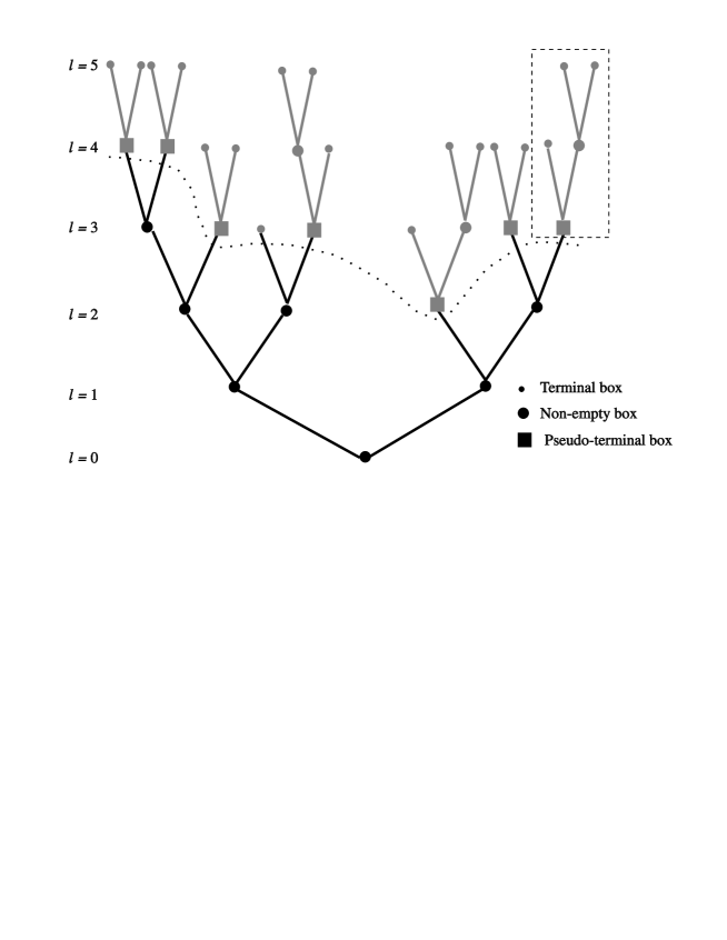
Figure 1: Example of types of boxes for a binary tree. Upper (gray) and lower (black) parts of the tree are depicted (up to the 5^th level). The dashed rectangle encloses one of the ‘sub-trees’ belonging to a processor’s domain.

The parallel tree-setting is then executed in two steps, the first step for the construction of the lower tree and the second one for that of the upper tree, as described in the following Sections.

3.1.1 Lower tree setting

In the first step, the particles are initially distributed at random to the PEs, i.e. without any correlation with their spatial location. Then, the PEs start building the tree, working on lower boxes, according to the recursive procedure described in Sect. 2. They consider, at the same time, the same box but dealing, of course, only with their own particles. This phase of the tree setting stops at PTERM boxes (instead of at terminal ones, as it is done in the serial version) where no more ‘branches’ are set up. In order to obtain an efficient parallel execution, the evaluation of the multipolar coefficients of (lower) boxes is done directly, i.e. by means of summations running over the set of particles contained, rather than by the recursive formulas involving the sub-boxes coefficients.

To attain the maximum data-locality, each PE keeps a copy of the tree structure in its own local memory. This makes that, in the tree-traversal stage, the reading access to lower boxes data will not be slowed down continuously by the inter-processors data transfer, which is one of the performances bottlenecks of codes running on distributed memory parallel computers. Note also that the amount of local storage needed to this part of the tree scales like the number of lower boxes, that is like $\sim\tau\log\tau$, being $\tau\sim N(kp)^{-1}$ the total number of PTERM boxes. Thus, the memory occupation for each local copy of the lower tree scales, conveniently, like the number of particles per processor. During the current step, the large number of particles in lower boxes (provided that $k$ is sufficiently great), together with the random particle distribution to the PEs, ensures a good work-load balancing.

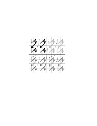
Figure 2: Example of PTERM boxes inspection order, for a uniform particle distribution in 2-D. The boxes are on the 3^rd level of the spatial subdivision and each pattern corresponds to a different processor’s domain (among 4 PEs), while the dashed arrows indicate the ‘jumps’ along the path.

At this point a suitable re-distribution of the particles (for an efficient tree-traversal) is performed ‘on the fly’ by exploiting our recursive way to set up the logical tree structure. Actually, such recursive approach, together with the technique used in mapping the particles’ coordinates (see Fig. 8), leads to a particular order in which the PTERM boxes are met. Such order corresponds to a one-dimensional path connecting a PTERM box to another spatially adjacent in a self-similar fashion (see Fig. 2). Though similar to that used by WS, the order is obtained in a substantially different way, as discussed in Appendix A.

This order is such that, by cutting the path into $p$ contiguous pieces with the same ‘length’ and then assigning to the $i$-th PE the particles contained into all the PTERM boxes in the $i$-th piece, one obtains a particularly efficient DD. Indeed, it is characterised by having most of sub-domains compact in space .

The particles assignement is performed every time a PTERM box is met. Moreover, other than the particles contained, also the data regarding the box are stored into the local memory of the PE. For this reason, it is necessary that the pointer in the parent box pointing to the PTERM one, includes also the information about which PE owns this latter. This way, any other PE can easily accede to the box data. The information is included within the pointer itself by constructing the full-address of the PTERM box, as described in Appendix B.

As in WS, we found that a good load-balancing can be attained if one ‘measures’ the path length in terms of the computational loads of the PTERM boxes, defining such quantity as the sum of the ‘weights’ of all the particles inside them, being the particle weight proportional to the number of bodies (both particles and boxes) whose force on it has been evaluated during the tree-traversal of the previous time step.

An important difference with respect to the WS’ method is that in our scheme the DD is performed via a (PTERM) boxes distribution to the PEs, rather then by directly distributing particles, and this means an easier parallel tree construction of the sub-trees in comparison with the HOT method. In this latter, in fact, there are several complications in setting up the local parts of the tree, such as: the ‘broadcasting’ of branch boxes, the inter-processor exchange of data regarding particles sited at the border of sub-domains, etc. In Fig. 3 an example of particles distribution to 4 PEs is plotted for a non-uniform case.

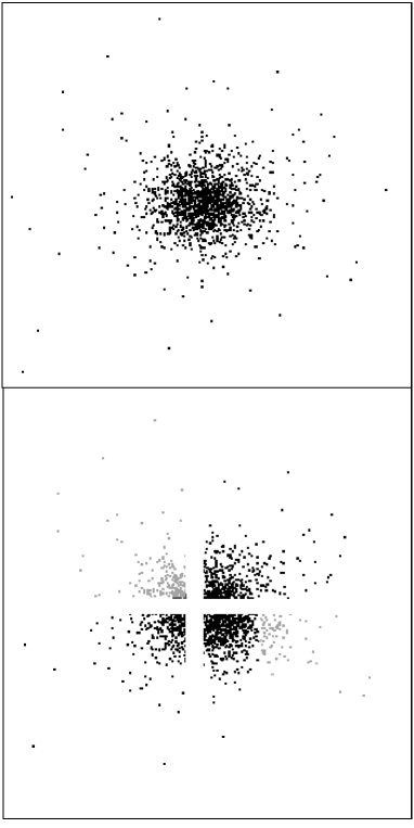
Figure 3: Example of domain decomposition among four PEs, for a cluster represented with 16,384 particles. Top: ‘section’ of the 3-D particles distribution lying on the $yz$ plane. Bottom: the sections of the 4 sub-domains have been spaced for clarity; note how one of them (the grey one) is not completely compact.

3.1.2 Upper tree-setting

The second step is the construction of the remaining upper part of the tree, which is performed according to the same recursive procedure used for lower boxes but, in this case, every PE works independently and without synchronism, starting every time from each PTERM box in its own domain. Every PE will store, in its local memory, the logical and data structure of all the sub-trees whose roots are given by such boxes. For example, in Fig. 1, the PE owning the rightmost PTERM box, will set up the sub-tree enclosed within the dashed rectangle. Another difference, in comparison with the lower tree setting, is that all the pointers box $\rightarrow$ sub-box adopt the full-addressing, because, in principle, any box could be required by other processors during the tree-traversal.

3.2 Parallel tree-traversal

In this stage, each PE uses exactly the same recursive procedure usually adopted in serial tree-codes (see e.g. Hernquist H (1987)) to evaluate the forces acting on the particles though, of course, only on those belonging to its domain.

At the beginning of this phase, such domain includes both the whole lower tree and those sub-trees whose roots are the PTERM boxes assigned to the PE. We can call all this set of boxes the initial locally essential tree (LET). This latter is not yet “complete”, in the sense that it does not include, yet, all the bodies that are necessary to evaluate the forces on the particles in the PE’s domain, lacking some of the upper boxes belonging to remote sub-trees (though they are the minority of all the required bodies, thanks to the spatially compact DD).

Anyway, the suitable addressing scheme adopted and the belonging of the boxes to the overall tree topology (as well as the recursive approach for the tree-traversal), allow us to perform the LET completion ‘at run time’. Given a particle belonging to a certain PE and given a box $B\in$ LET whose sub-boxes have to be handled: if a sub-box does not belong to the LET, as can be immediately recognized by Eq. 4, then (i) get all its data (and all its pointers) from the owning PE’s memory at the address given by Eq. 5, (ii) copy them into a free location of the local memory, (iii) change the pointer in $B$ to point this new local address. This way, the sub-box is included into the LET and when any other particle requires it, it is already found into the local memory. This mechanism minimizes the amount of inter-processor communications.

Note that the full-addressing mechanism makes remote data retrieval immediate, thanks to that the local sub-trees are portions of a single and global tree arrangement, unlike the orthogonal recursive bisection scheme (Warren & Salmon orb (1992)). In our opinion our addressing method is as ‘global’ as that used in WS, though easier to be implemented and with a lower computational overhead, as we will see.

4 Results

The efficiency of the parallelization method has been checked by analysing the performances for a single evaluation of the forces on a set of particles. Such evaluation includes one tree-setting (including DD) and one tree-traversal step, as well as all the necessary inter-processor communications and remote accesses (LET completion), without the time integration of trajectories. Indeed, it is known that most of the CPU-time used by a simulation of large self-gravitating systems is spent in the computation of the gravitational interactions. Usually this latter takes at least 80% of the total CPU-time, while the time advancing of particles’ dynamical quantities (position, velocity, etc.) takes just $\sim$ 10%, because its computational cost scales like $N$. This cost is even smaller for low-order time integration schemes, like those generally used in conjunction with tree-codes. Moreover, it is generally very simple to parallelize time integration methods, because the time advancing of a particle is independent of that of the others and the corresponding work-load is, normally, very homogeneous. For this reason our tests involve the forces computation only, which indeed represents the key problem to overcome for getting a good parallelization.

Nevertheless, one has to be careful when time integration algorithms adopt individual time steps (that is a desirable feature when dealing with self-gravitating systems with a wide range of time scales), because they imply a force evaluation which is mostly performed on a subset of the entire set of particles. We discuss this problem in Appendix C.

All the tests were performed on a set of $N=128$K equal mass ($m$) particles distributed according to the Plummer profile (known to fit acceptably globular clusters, at least in regions not too far from the center, see Binney & Tremaine binney (1987)) $\rho(r)=\rho_{0}(1+r^{2}/r_{c}^{2})^{-5/2}$, within a sphere of radius $R$ such to include a particles total mass, $M=Nm$, such that $M=0.995\times M_{\infty}$, where $M_{\infty}=\int_{0}^{\infty}4\pi r^{2}\rho dr$. The core radius is chosen as $r_{c}=6\times 10^{-2}R$, while $\rho_{0}=3M_{\infty}(4\pi r_{c}^{3})^{-1}$ is the central density. This is a highly non-uniform distribution, being $\rho_{0}/\rho(R)\sim 10^{6}$ (see Fig. 4).

For the box-particle force evaluation we used multipolar series truncated at the quadrupoles, and the original BH ‘opening’ criterion with different values for the open-angle parameter $\theta$. The maximum number of particle in PTERM boxes (see Sect. 3.1) was set equal to $16\times p$, this value giving the best performances for any number of PEs ($p$), as we checked. The tests ran on a Cray T3E and regarded our parallelization method implemented by means of PGHPF/Craft directives.

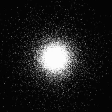
Figure 4: The clustered set of 128K particles used in the tests.

4.1 The performances

The good efficiency of the parallelization approach described in previous Sections is basically shown by three facts: i) a behavior of the relative speedup close to the ideal one (linear in $p$); ii) a low unbalancing of the work-load; iii) a low parallelization overhead.

Figure 5: Speedup for the force evaluation on $N=128K$ particles (Plummer profile). Bottom: code speed vs. the error on the forces $\delta a/a$ at the 90% percentile (i.e. such that 90% of particles have a force affected by a relative error $\leq\delta a/a$) for various number of PEs ($p$) and different values of $\theta$, as labeled. Top: the speedup with respect to a single PE run (in the $\theta=0.7$ case) plotted for the overall force evaluation and for the tree-traversal (t.t.) only.

The good overall code scalability is shown in the upper panel of Fig. 5. It appears to be rather good for $p\leq 16$ (i.e. $N/p\geq 8192$). For more than 16 PEs, the performances start to degrade because of the too small number of particles per PE: with $p\leq 32$ one has $\leq 4096$ particles per PE that makes the tree-code not that efficient in itself. To give immediate indications of how fast the calculations are for a given accuracy, we show in the lower panel the absolute speed of the code versus the relative error on the forces evaluation. The relative error on the evaluation of the force (per unit mass) on a particle – due to the use of the truncated multipolar expansion for the box satisfying the opening criterion – is defined as: $\delta a/a\equiv|a_{\rm tc}-a|/a$, where $a$ is the magnitude of the acceleration evaluated by means of the ‘exact’ particle-particle summation, and $a_{\rm tc}$ denotes the magnitude of the acceleration calculated via the tree-code.

The computational work-load is well balanced among the PEs. A natural way to quantify the load unbalancing, $u$, is via the formula $u=(t_{\rm max}-t_{\rm min})/<\!\!t\!\!>$, where $t_{\rm max}$ and $t_{\rm min}$ are, respectively, the maximum and the minimum CPU-time spent by the PEs to perform a given procedure and $<\!\!t\!\!>$ is the averaged CPU-time. From Fig. 6, we can see that, for a sufficiently high number of particles per PE (say for $N/p\geq 8,000$) we have a quite low $u$, that is less than 10% for the tree-setting and always less than 6% during the tree-traversal, demonstrating the efficiency of the DD. Only for $N/p\sim 4,000$ the unbalancing becomes unacceptable ($>50$%).

Figure 6: Load unbalancing parameter ($u$) for a single force evaluation with $\theta=0.7$. Solid line: for the tree-setting stage; dotted line: for the tree-traversal.

Last, but not least, we can see in Table 1 that the parallelization overhead takes only 3.2% of the total CPU-time in a 8 PEs run. Moreover, as we verified, this percentage increases significantly only when $N/p<8,000$. Thus, in optimal conditions the ‘surplus’ of CPU-time specifically needed to make the parallelization operative (in our case spent by the DD plus the LET completion) is almost negligible. This point is crucial in order to state that a parallel code is really efficient.

Indeed, even in a distributed memory context one can get a highly scalable tree-code with a good work-load balancing, using just an absolutely banal DD. In fact, the load balancing can be achieved by means of a ‘dynamical’ distribution of the particles to the PEs (see Singh et al. singh (1995)), tolerating a great deal of communications and remote accesses. Following this approach, we implemented another parallel version of the tree-code obtaining a good speedup scaling and a low load unbalancing on the T3E, but the communications overhead heavily affected the absolute performaces making it not convenient for practical use (see Capuzzo-Dolcetta & Miocchi cdm-ssc97 (1998), cdm-cpc (1999)).

Table 1: Code CPU-time consumption with 8 PEs, 128K particles and $\theta=0.7$. Italic: parallelization overhead.

Code section	sec	%
tree-setting	$1.4$	$6$
domain decomposition	$0.1$	$0.5$
tree-traversal	$21$	$94$
LOWER tree-traversal	$3.3$	$15$
UPPER tree-traversal	$18$	80
LET completion	$0.6$	$2.7$
total	$22.4$	$100$

Finally, the code memory usage requires roughly 1 Kbyte per particle. For instance, more than $10^{7}$ particles can be handled by 128 processors having 128 Mbyte each. Such amount of particles can be furtherly increased in a more optimized message passing implementation.

4.2 Comparisons with other codes

To make really significant comparisons of the performances of different tree-codes, one should ensure the forces computation be done with the same accuracy and on the same set of particles. Of course, such performances depend also on the opening criterion adopted, because at a given accuracy and with a given set of particles, different opening criteria can give different amounts of interactions to evaluate on a particle, thus giving different computation speeds. Therefore, if one wants to compare specifically the efficiency of the parallelization approach, then the tests should be done with the same opening criterion too.

Unfortunately, it is often very difficult to make such conditions hold with the tree-codes available in the literature. For this reason we decided to compare codes speed at a given amount of computational work done to evaluate forces. This makes the comparison independent of: the particles distribution, the number of particles, and the accuracy (i.e. the opening criterion and its parameters). In tree-codes the amount of numerical work done on a given particle, $w_{i}$, is naturally quantified as the number of ‘interactions’ evaluated to estimate the force on it (as in the particle work-load definition of Sect. 3.1.1), namely the total number of bodies (both boxes and single particles) of which the tree-code evaluates the force they exert on the particle itself (in a particle-particle method one would have $w_{i}=N-1$).

In Fig. 7 we plotted the error on the forces evaluation ($\delta a/a$), versus the averaged computational work, $<\!\!w\!\!>=(\sum_{i}w_{i})/N$, needed by our code to evaluate the forces on the set of $N=128$K particles above-described. This allows us to compare ‘honestly’ our code performances with those of other codes.

Figure 7: Relative error on forces evaluation (at 90% percentile) versus the averaged computational work, using the BH opening criterion. The corresponding values for the open-angle parameter $\theta$ are labeled.

In Springel et al. (gadget (2000)) the authors tested their tree-code (GADGET) on a Cray T3E. They give speed measurements for a rather clustered cosmological distribution, using the BH opening criterion with $\theta=1$. In such conditions their code gives $\delta a/a\sim 3.5\times 10^{-2}$ at 90% percentile, with $<\!\!w\!\!>\simeq 200$ interactions per particle. From Fig. 7 we can see that, with the Plummer distribution we used, the closest value for $<\!\!w\!\!>$ is achieved for $\theta=1.2$, which gives $<\!\!w\!\!>\simeq 230$ interactions per particle and corresponds to an accuracy of $\delta a/a\sim 3\times 10^{-2}$. Such accuracy is obtained in a run that, using e.g. 8 PEs, is performed with a speed of $15,000$ particles/sec (as shown in the lower panel of Fig. 5). Note that such run includes, apart from the tree-traversal, also the tree-setting and all the overhead needed to a parallel execution. At the same conditions, but performing only the tree-traversal stage, GADGET has a lower speed: about $13,000$ particles/sec (with 8 PEs). It is worth noting that it shows a load unbalancing of about 19% with $N/p\sim 3\times 10^{4}$, while our code exhibits $u\sim 4$% with the same ratio $N/p$. One has to say, finally, that GADGET has been implemented using message passing instructions, certainly a more suitable approach with respect to that we adopted (see next Section).

Another comparison can be done with the parallel code illustrated in Dubinski (dubinsky (1996)). In this case the code ran on a Cray T3D and the author employed a more efficient modified BH opening criterion (Barnes barnes (1994)). Anyway, the rapidity of the code is given both in terms of the total computational work ($N<\!\!w\!\!>$) performed in one second, and in terms of particles per second. With 16 PEs such code evaluated about $3\times 10^{6}$ interactions/sec, corresponding to $6,000$ particles/sec, for a forces computation performed on a cluster with $N=1.1$M particles. This means that the code spent $t\simeq 180$ sec in that run. Hence, being $N<\!\!w\!\!>/t\simeq 3\times 10^{6}$, it handled $<\!\!w\!\!>\simeq 500$ interactions per particle. With our tree-code such $<\!\!w\!\!>$ corresponds to an accuracy of about $\delta a/a\sim 4\times 10^{-3}$ (Fig. 7), and so it is performed at $\sim 13,000$ particles/sec with 16 PEs (Fig. 5). Of course, our speedup factor of $2$ is partially due to the improved performances of the T3E compared with the T3D, even if the direct message passing approach used by the author is more efficient then the use of the PGHPF compiler.

4.3 Remarks about the implementation

The use of PGHPF/Craft directives is certainly not the best way to implement a parallel tree-code on a distributed memory architecture, but we did so in order to obtain quickly a ready-to-use version. Indeed, the directives permit just to distribute in a simple way loop iterations to the PEs, as well as the elements of shared arrays to their local memory, without using explicit message passing routines.

The highest price to pay for such simplicity, is that the way message passing operations are actually performed cannot be controlled and optimized. In our specific case, each PE has to copy all its local upper tree to logically shared arrays, in order to enable the other PEs to accede to it during the tree-traversal. This means a considerable waste of memory (and communications), which can be avoided in a direct message passing implementation, so to reduce furtherly the parallelization overhead.

Similar storage and clock time wastings are due also to that the PGHPF compiler is generally not capable to recognize local references within a shared array, which are handled as if they were remote instead. Anyway, we experimented also a slow local referencing, due to a non optimal cache-memory managing. For these reasons, our next goal is the development of an MPI version, which would also be easily implementable on different distributed memory platforms.

Finally, we have also carried out an implementation suitable for running on a shared memory computer. In this case, of course, the DD has to take into account only the work-load balancing and a ‘dynamic’ particles distribution can be adopted during the tree-traversal. Anyway, it turns out to be worth subdividing the tree into upper and lower boxes for a balanced tree-setting. Such implementation was carried out using OpenMP directives on a SUN Enterprise 4500 HPC machine, with 14 PEs. The results are very good and, given the same parameters, we verified a $40$% speedup in comparison with the T3E PGHPF implementation.

Appendix A Particle mapping

Particles’ locations are mapped converting each coordinate, $x_{i}$, $i=1,2,3$, into an integer triple $q_{i}=\lfloor x_{i}\times 2^{l_{\max}}/L\rfloor$, where $\lfloor...\rfloor$ indicates the truncation to an integer, $L$ is the root box’ size and $l_{\max}$ is the maximum subdivision level a priori allowed. Then $q_{1,2,3}$ are combined into an integer number (the ‘key’) $Q\in[0,8^{l_{\max}}-1]$, which is defined as:

$$Q = \sum_{l=1}^{l_{\max}}\left[\mbox{mod}(\lfloor q_{1}/k_{l}\rfloor,2)+2\times\mbox{mod}(\lfloor q_{2}/k_{l}\rfloor,2)+\right.$$ (1)

$$\left.+4\times\mbox{mod}(\lfloor q_{3}/k_{l}\rfloor,2)\right]^{k_{l}^{3}},$$

where $k_{l}=2^{l_{\max}-l}$. Despite its complicated definition, $Q$ can be rapidly evaluated by means of direct bit manipulation routines available both in FORTRAN and in C.

Given a particle’s key, it is possible to determine quickly whether it belongs to a box or not, in a recursive fashion. Let us indicate the key binary representation as $Q\equiv\{b_{3l_{\max}-1}b_{3l_{\max}-2}\cdot\cdot\cdot b_{2}b_{1}b_{0}\}_{2}$, then: known that the particle belongs to a certain box at the level $l$ of the spatial subdivision, at the level $l+1$ such particle will belong to the $i$-th sub-box ($0\leq i\leq 7$) which is identified by the octal digit $i\equiv\{b_{k+2}b_{k+1}b_{k}\}_{2}$. This latter is made up of the three adjacent bits of $Q$ from position $k=3(l_{\max}-l-1)$ to the left. For $l=0$ any particle is enclosed in the root box. See the example in Fig. 8.

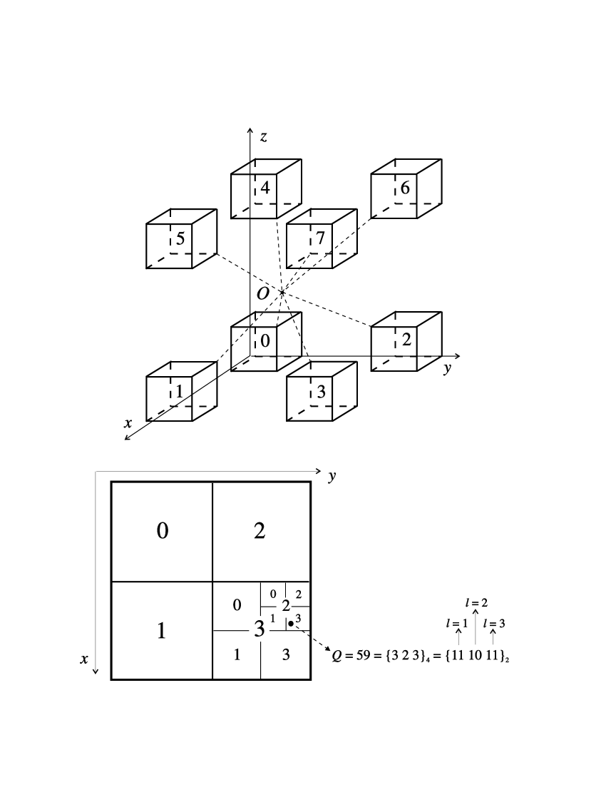
Figure 8: Top: a parent box (centered at $O$), has been “opened” to show the numbering of its sub-boxes (in 3-D), which allows to identify, by suitably extracting octal digits from the key $Q$ of a particle, the sub-box which it belongs to. Bottom: example of a particle mapping shown in the 2-D case for simplicity; in this case ($l_{\max}=3$) each sub-box enclosing the plotted particle, is recursively identifies by base 4 digits made up of 2 bits.

Each key needs $3l_{\max}$ bits to be handled. We used two long-integers (i.e. $16$ bytes), thus allowing $l_{\max}\leq 42$, which is sufficient for most applications. Note that the evaluation of the keys of all the particles, with a computational cost of order $O(N)$, can be done just once, before the tree setting starts.

The mapping method described in WS is similar, to some extent, to that above-illustrated, but in that case the authors do not use pointers to reproduce the tree topology, they rather use the particles’ keys themselves (evaluated similarly as in Eq.1) plus a hashing function to build an addressing space for all the boxes. Roughly speaking, in order to reduce the huge number of a-priori possible keys (e.g. in 3-D there are $8^{l_{\max}}$ possible values for $Q$), they truncate the keys binary representation, replacing the information losted this way by means of linked lists. In the authors opinion this presents mainly the following advantages: i) it permits a direct access to any boxes, without needing a tree-traversal; ii) in a distributed memory context, it gives a unique addressing scheme for the boxes, independently of which PE owns them. We think that the advantage in point i) is not important in our implementation because, as we have seen, any procedure involving the tree structure is performed recursively. A direct access to a box does not really speed up the execution; moreover, in WS’ method the accesses are not really direct (expecially at upper levels) due to the presence of linked lists. As far as point ii) is concerned, also in our parallel version there is an addressing scheme which allows data in any sub-domain to be globally referenced (see Sect. 3.1 and Appendix B).

Appendix B Construction of a global addressing scheme

Given the binary representation of baddr$\equiv\{b_{m-1}b_{m-2}\cdot\cdot\cdot b_{1}b_{0}\}_{2}$ that is the address location of an upper box within the i-th PE’s local memory, we define the box full-address as the $s$-bit number (being $s$ the bit size of integer variables, excluding the bit used for the sign):

$$\mbox{\tt faddr}\equiv\{100\cdot\cdot\cdot 0b_{m-1}b_{m-2}\cdot\cdot\cdot b_{1}b_{0}c_{7}c_{6}\cdot\cdot\cdot c_{1}c_{0}\}_{2},$$ (2)

being i$\equiv\{c_{7}c_{6}\cdot\cdot\cdot c_{1}c_{0}\}_{2}$. Note that the leftmost bit, in position $s-1$, is set to 1 in order to indicate that the box pointed is an upper one. Note also that 8 bits are used for i, allowing $p\leq 256$. To make the full-address be a single integer number it is necessary that $m+8<s$. Hence with 8-bytes integers ($s=63$) the local addressing is limited by $2^{55}$ that is sufficient for any purpose.

In FORTRAN such ‘bit concatenation’ can be easily carried out this way:

$$\mbox{{\tt faddr = Ior(Ior(Ishft(baddr,8),i),mask)}},$$ (3)

where mask$=2^{s-1}$. Inversely, given the full-address of a box, the following bit manipulation instructions give the address in the local memory of the i-th processor which it belongs to:

i $$= \mbox{{\tt Iand(faddr,mask2)}},$$ (4)

baddr $$=$$ Ishft(Iand(faddr,mask1),-8) (5)

being mask1$=$mask$-1$ and mask2$\equiv 255$.

Appendix C Parallel time integration

As far as the time integration is concerned, when the time advancing algorithm adopts individual time steps, at a given time the forces are evaluated only on a sub-set of all the particles. This leads to a work-load as more unbalanced as the sub-set is smaller. We experimented various possible solutions for such problem, in particular in the case of the leapfrog algorithm with the block-time scheme (Porter porter (1985); Henquist & Katz HK (1989)). According to this scheme, the $i$-th particle occupies the ‘time bin’ $b_{i}\in\{0,1,2,...,b_{\rm max}\}$, in the sense that it gets a time step $\Delta t_{i}=\tau/2^{b_{i}}$, where $\tau$ is the maximum time step allowed (usually a fraction of a significant time scale for the system). The simulation time ($t$) is advanced by the minimum time step used and, at a given $t$, the accelerations are evaluated only on synchronized particles, i.e. on those whose acceleration was calculated last time at $t-\Delta t_{i}$ (at $t=0$ all the particles accelerations are evaluated). According to some rules, $\Delta t_{i}$ can also change with time.

First, we found convenient to set the maximum a priori possible bin not that high, say $b_{\rm max}<6$, so to avoid bins with too few particles within. This choice is also recommendable because of the intrinsic non-symplectic nature of the individual time step leapfrog. Indeed, every time a particle changes its bin, a lost of time symmetry occurs, leading to instability and to a long term energy drift. Furthermore, good results are obtained if, at a given instant, one assignes to synchronized particles a weight ($w$) much greater than those assigned to the others. One could be even tempted to set $w=0$ for non-synchronized particles because no work will be done, in the current step, to update their accelerations. Nevertheless, this would give rise to a very unbalanced work-load during the tree-setting, because wide sets of PTERM boxes (containing zero-weight non-synchronized particles) may be assigned to the same PE, forcing it to build large portions of the upper tree. We found that a good compromise is to multiply the weight of the currently synchronized particles – initially estimated as described in Sect. 3.1.1 – by the factor $N/s$, being $s$ the number of these latter.

This mantains the unbalancing comparable with that of the single force evaluation on all the particles, also in those highly dynamic situations in which the accelerations of the particles moving through very dense region (like for pairs of stars during close encounters occurring within the core of a globular cluster) need to be frequently updated.

References

- (1) Barnes, J.E. 1994, in Computational Astrophysics, eds. J. Barnes et al. (Berlin: Springer-Verlag)
- (2) Barnes, J.E., & Hut, P. 1986, Nature 324, 446
- (3) Binney, J., & Tremaine, S. 1987, Galactic Dynamics (Princeton, USA: Princeton University Press)
- (4) Capuzzo-Dolcetta, R., & Miocchi, P. 1998, in Sciences & Supercomputing at CINECA, 1997 Report, ed. M. Voli (Bologna: CINECA), 29
- (5) Capuzzo-Dolcetta, R., & Miocchi, P. 1999, Computer Phys. Communications, 121-122, 423
- (6) Dubinski, J. 1996, New Astronomy, 1, 133
- (7) Hernquist, L. 1987, ApJS 64, 715
- (8) Hernquist, L., & Katz, N. 1989, ApJS 70, 419
- (9) Lia, C., & Carraro, G. 2000, MNRAS, 314, 145
- (10) Pal Singh, J., Holt, C., Totsuka, T., et al. 1995, Journal of Parallel and Distributed Computing, 27, 118
- (11) Porter, D. 1985, Ph.D. thesis, University of California (Berkeley, USA)
- (12) Springel, V., Yoshida, N., & White, S.D.M. 2000, submitted to New Astronomy (astro-ph/0003162)
- (13) Warren, M.S., & Salmon, J.K. 1992, Astrophysical N-Body Simulations Using Hierarchical Tree Data Structures, in Supercomputing ’92 (Los Alamitos: IEEE Comp. Soc.), 570
- (14) Warren, M.S., & Salmon, J.K. 1993, A Parallel Hashed Oct-Tree N-Body Algorithm in Supercomputing ’93 (Los Alamitos: IEEE Comp. Soc.), 12