Imaging of detached shells around the carbon stars
R~Scl and U~Ant through scattered stellar light
††thanks: Based on observations using the 3.6 m telescope of the
European Southern Observatory, La Silla, Chile.
We present the first optical images of scattered light from large, detached gas/dust shells around two carbon stars, R~Scl and U~Ant, obtained in narrow band filters centred on the resonance lines of neutral K and Na, and in a Strömgren b filter (only U~Ant). They confirm results obtained in CO radio line observations, but also reveal new and interesting structures. Towards R~Scl the scattering appears optically thick in both the K and Na filters, and both images outline almost perfectly circular disks with essentially uniform intensity out to a sharp outer radius of 21. These disks are larger – by about a factor of two – than the radius of the detached shell which has been marginally resolved in CO radio line data. In U~Ant the scattering in the K filter appears to be, at least partially, optically thin, and the image is consistent with scattering in a geometrically thin (3) shell (radius 43) with an overall spherical symmetry. The size of this shell agrees very well with that of the detached shell seen in CO radio line emission. The scattering in the Na filter appears more optically thick, and the image suggests the presence of at least one, possibly two, shells inside the 43 shell. There is no evidence for such a multiple-shell structure in the CO data, but this can be due to considerably lower masses for these inner shells. Weak scattering appears also in a shell which is located outside the 43 shell. The present data do not allow us to conclusively identify the scattering agent, but we argue that most of the emission in the K and Na filter images is to due to resonance line scattering, and that there is also a weaker contribution from dust scattering in the U~Ant data. Awaiting new observational data, our interpretation must be regarded as tentative.
Key Words.:
Stars: carbon –circumstellar matter –Stars: individual: R Scl, U Ant – Stars: mass-loss1 Introduction
Low, and intermediate-mass stars populate the asymptotic giant branch (AGB) after central He-burning. During this stage of evolution they are known to experience intense mass loss in the form of a cool, slow, and essentially spherically symmetric wind (Olofsson olofsson96b (1996)). The mass loss eventually becomes so large that it, rather than the nuclear burning, determines the evolutionary time scale of these stars. This limits the AGB life time, and e.g. provides an explanation to the discrepancy between the observed and calculated luminosity functions of stars on the horizontal branch and on the AGB in globular clusters (Renzini renzini (1981); Iben iben (1981)). The mass loss also makes an important contribution to the enrichment of the interstellar medium in terms of nuclear-processed material and dust particles (Busso et al. busso (1999)). Considering this, it is unfortunate that our knowledge of the details of the mass loss and the mechanism behind it is so limited.
The formation of circumstellar envelopes (CSEs) of gas and dust around AGB stars is a consequence of the mass loss. The main constituent of the outflowing gas, H2, is generally not observable, despite being excited by shocks in a few particular circumstances, notably young post-AGB objects and planetary nebulae (Beckwith et al. beckwith (1978); Weintraub et al. weintraub (1998)). Standard stellar atmosphere chemistry theory predicts that the first molecule to form as the gas cools is CO (Glassgold glassgold96 (1996)). Depending on the star being O-rich (i.e., [C]/[O]1) or C-rich ([C]/[O]1) the CO molecules consume all the available carbon or oxygen atoms, respectively. This leads to a drastically different molecular chemistry and dust composition in the CSEs around these two types of AGB stars. Direct measures of the gas, the principal component in terms of mass of a CSE, are provided by radio line emission of these minor molecular constituents. Of particular importance for the study of the mass loss properties are observations of CO for both O- and C-rich stars (Olofsson et al. olofsson96 (1996)).
The temporal variation of the mass loss rate is to a large extent unknown. This applies to all time scales from the pulsation period to the full time scale for the AGB-phase. For the shortest time scales we are limited by the spatial resolution of the observations, while for the longest time scales we lack suitable observational probes. On the intermediate time scales (102–104 yr) there is now growing evidence for substantial variations in the mass loss rate, e.g., detached CO and dust shells have been detected around a number of AGB and post-AGB stars (Olofsson et al. olofsson (1990), olofsson96 (1996); Lindqvist et al. lindqvist (1996), lindqvist99 (1999); Waters et al. waters (1994); Izumiura et al. izumiura (1996), izumiura97 (1997); Hashimoto et al. hashimoto (1998); Speck et al. speck (2000)), and multiple-shell structures have been seen in scattered light towards IRC+10216 and a number of post-AGB objects (Harpaz et al. harpaz (1997); Kwok et al. kwok (1998); Sahai et al. sahai (1998); Mauron & Huggins mauron99 (1999)). Interferometric observations of the CO shell around the carbon star TT~Cyg provide a splendid result (Olofsson et al. olofsson98 (1998), olofsson00 (2000)). The shell is large (radius 35″), geometrically thin (average width 2.5″), and remarkably spherical (only 3% variation in radius). Similar results have been obtained for the carbon star U Cam (Lindqvist et al. lindqvist99 (1999)). A significant fraction of the AGB-stars has excess emission at 60 m (and 100m) in the IRAS PSC, which has been interpreted as a sign of detached envelopes, and hence variable mass loss (Willems & de Jong willems (1988); Chan & Kwok chan (1990); Zijlstra et al. zijlstra (1992)). However, in most cases this excess can probably be attributed to interstellar cirrus emission (Ivezic & Elitzur ivezic (1995)). Thus, there remain only a few, clear examples of highly episodic mass loss on the AGB. The exact origin of the detached shells is still uncertain. They could be rare examples of ‘thermal pulse’-induced mass loss eruptions (Olofsson et al. olofsson (1990); Schröder et al. schroder (1999)), but effects of interacting winds cannot be excluded, with the CO shells being the shock zones (Olofsson et al. olofsson00 (2000); Steffen & Schönberner steffen (2000)).
R~Scl and U~Ant are among the few carbon stars with extended, detached shells detected in CO radio lines (Olofsson et al. olofsson (1990), olofsson96 (1996)). For R~Scl, the CO brightness maps show a marginally resolved detached shell (radius 10″), which appears to have detached fairly recently (103 yr). Detections of other molecules, such as HCN, CN and CS, point to a dense shell where these molecules are still relatively abundant and excited (Bujarrabal & Cernicharo bujarrabal (1994); Olofsson et al. olofsson96 (1996)). The CO emission from U~Ant shows both a ‘normal’ CSE and a detached shell (radius 40″). The latter appears to have an overall spherical symmetry, but its brightness distribution is not smooth, suggesting clumpiness at some level in the density distribution, as well as a marked decrease in the CO intensity towards the south-west. Izumiura et al. (izumiura97 (1997)) deconvolved IRAS 60 and 100 m observations of U~Ant, and they inferred the existence of two extended dust shells. The (uncertain) size of the inner shell, apparent as a brightness distribution broader than the PSF, is consistent with that of the detached CO shell. The outer shell has an inner radius of about 3′ and no CO counterpart.
The interpretation of the CO emission is hampered by the fact that it depends on the excitation as well as on the chemistry (particularly the photodissociation by the interstellar radiation field) of the CO molecules. Hence, the relationship between the density distribution (and consequently the mass loss history) and the CO brightness distribution is uncertain. Also, the lack of an interferometer in the southern hemisphere prevents us from obtaining CO radio line observations of R~Scl and U~Ant with the high resolution achieved for the northern sources TT~Cyg (Olofsson et al. olofsson98 (1998), olofsson00 (2000)) and U~Cam (Lindqvist et al. lindqvist (1996), lindqvist99 (1999)). Infrared emission from dust is the only probe of CSEs which is not destroyed by the interstellar radiation field and therefore these observations trace the long-term history of mass loss. However, the data are often of very poor spatial resolution. Hence, there is an urgent need for other ways of observing the detached shells. In this paper we present the first optical images of the envelopes around R Scl and U Ant, which we infer to be the result of stellar light scattered in atomic resonance lines and/or by dust particles. These high spatial resolution data will allow us to further study the morphology and structure of the shells. The feasibility of optically observing CSEs was first shown spectroscopically by Bernat & Lambert (bernat (1975)). They used a method whereby normalized on–star spectra are subtracted from off–star spectra, to reveal the faint circumstellar emission; this technique was used and developed further by Mauron & Caux (mauron92 (1992)), Plez & Lambert (plez (1994)), and Gustafsson et al. (gustafsson (1997)).
2 Observations and data reduction
2.1 Observations
The imaging observations presented in this paper were done primarily in narrow (5 nm FWHM) filters centred on the resonance lines of NaI (589.0 nm and 589.6 nm; the D lines) and KI (769.9 nm), using the EFOSC1 and EFOSC2 focal reducer cameras on the ESO 3.6m telescope in 1994 and 1999, respectively. We used narrow filters to reduce the amount of direct photospheric light in the images, and thereby increase the contrast of any circumstellar line scattered light. Even narrower filters were considered, but they would introduce new unwanted difficulties in the observations, such as the temperature dependence of the transmitted wavelengths, and wavelength shifts over the image that are greater than the filter widths (produced by the large difference in angle at which light passes through the filter from one side of the field to the other in a parallel beam instrument). During the second observing run, we also observed U~Ant in other filters, which contain no strong resonance lines (Strömgren v, =410.0 nm, =18 nm; Strömgren b, =468.0 nm, =20 nm; and Gunn z, =900 nm, =20 nm, approximately). In Table 1 we summarize the observations done during the two observing runs.
|
The stellar fluxes turned out to be typically four orders of magnitude higher than the circumstellar scattered light fluxes. A coronograph is therefore essential, and we used an opaque dot placed on a glass plate in the focal plane of the EFOSC instruments. By using this method, most of the photospheric light that is scattered in the Earth’s atmosphere is avoided. However, even the use of a coronographic mask is not enough, and an additional method is required in order to subtract the remaining direct photospheric radiation. This additional method is based on the observation of template stars, i.e., stars with about the same magnitude and spectral type as the target stars, but without CSEs. These template star images are subtracted from the target star images during the reduction. Due to atmospheric variations, the stellar profiles change during the night. Therefore, we observed several template stars well distributed throughout the full runs. Standard stars were only observed during the second observing run.
The first images in circumstellar scattered light were obtained during observations carried out in 1994 at a test run with the ESO 3.6m telescope and the EFOSC1 ‘focal reducer’-type camera. The pixel plate scale was 061, and exposure times of only a few minutes were sufficient for the detections. Three bright carbon stars with detached shells detected in CO radio lines (R~Scl, U~Ant, S~Sct) were chosen as targets during this test run. Emission due to circumstellar scattering in extended envelopes was found for two of them, R~Scl and U~Ant. These detections are, however, of relatively low S/N-ratio. Around S Sct we found, using a polarimetric technique, an extremely faint and diffuse shell at very low S/N-ratio. This test run turned out to be the first success after a series of attempts in previous years with other telescopes [the 2.5m Nordic Optical Telescope (NOT) and the MPG/ESO 2.2m telescope]. Successful spectroscopic observations were performed with the ESO CAT/CES-system by Gustafsson et al. (gustafsson (1997)) demonstrating the presence of circumstellar resonance line scattering around R~Scl and other stars. The observational problem of imaging the circumstellar shells is clearly their faintness, which makes the stellar light scattered in the Earth’s atmosphere and the telescope very problematic. The ESO 3.6m telescope was crucial to the outcome of the project. Apart from a large collecting area, it has an equatorial mounting. In alt-az telescopes, like the NOT and the ESO NTT, the rotation of the instrument during the observations smears out the spider diffraction pattern over the images. This results in a substantial loss of azimuthal information, rendering it difficult to make a detection of weak emission from an extended envelope.
Based on the successful observations during the test run, we continued in 1999 with the imaging of one of the stars, U~Ant, with the EFOSC2 camera. The pixel plate scale in EFOSC2 is 032. We detected again the emission from the envelope around U~Ant, in this case in several filters and with much higher S/N-ratio. During this second run, we also observed two stars with detached dust shells, U~Hya (Waters et al., waters (1994)) and R~Hya [the only O-rich source with a detected detached dust shell (Hashimoto et al., hashimoto (1998))], and one source with a possible detached dust shell, X~TrA (Izumiura et al. izumiura95 (1995)). In addition, we observed VX~Sgr, an M-type supergiant. We were not able to detect any circumstellar emission in these sources. Due to the complexity of the observations, there can be several reasons for this negative result. Normal envelopes, in which the density peaks close to the star, are very difficult to detect in scattered stellar light. It is worth noting that the circumstellar emission observed towards IRC+10216 is due to scattered interstellar light, and the central star is highly obscured (Mauron & Huggins mauron99 (1999)). Shells located close to the star, more extended (and therefore even fainter) shells (e.g., in S Sct), and the presence of the star in a crowded stellar field are other plausible reasons for the non-detections. We postpone the discussion of the tentative S Sct shell and the non-detections to a future paper.
2.2 Data reduction
The image reduction was done in two steps using IRAF. First, an ordinary CCD reduction (bias subtraction, flatfield correction, and cosmic ray removal) was performed. This resulted in images with some considerable distortions. In particular, the coronographic optics at the ESO 3.6m telescope was fairly crude, e.g., the focal plane obscuring spot masks are made on a glass plate that introduced optical distortions. Furthermore, the lack of an optimized apodising mask to remove the spider diffraction pattern on the images, resulted in two highly saturated stripes, corresponding to the segments of the spider, along the horizontal and vertical directions of the images, where the reduction is much more complicated. Therefore, the circumstellar emission detected in the various images shown in this paper is not reliable along these two directions. Some cleaning was performed in the images in order to remove field stars whose brightness could swamp the circumstellar emission.

Second, the template star subtraction was done (the template star images are first reduced as above and then median filtered in this process). One of the key aspects of these observations is the placement of the objects under the coronographic spot. This is a very difficult task and when doing the reductions we have realized that the stars were not positioned exactly under the centre of the coronographic mask, and therefore the positions of the stars are difficult to locate precisely. An accurate subtraction requires the target and template stars to be perfectly aligned, and so an indirect method had to be used to achieve this. We estimated the positions of the stars using their radial profiles along various position angles. We defined these positions as the middle points between two pixels (one on each side of the centre) with the same intensity level. We averaged the values obtained using different intensity levels and different radial profiles (along different position angles) to get a final location of the target and template stars.
Next in the reduction came the normalization of the template star images, i.e., normalizing the template star intensity to that of the target star. Again, the absence of peaks in the images made this task somewhat complicated. We normalized by a method of trial and error, using a radial range outside the innermost usable points (7 and 5 from the star centres in the reductions of the R~Scl and U~Ant images, respectively) of several radial profiles. The profiles of the target star and the template star are usually perfectly matched close to the coronographic mask after normalization. The addition of a small constant value to the template image was used to equalize the background light in the images due to the sky background. The inner points, where the intensity is much higher, are not significantly affected by this addition.
Finally, we subtracted the template star image from the target star image. This subtraction removes both the stellar and the background components from the target star image, leaving us only with the circumstellar emission. We have repeated this procedure using two template stars, in order to make sure that the observed circumstellar contributions are not artifacts produced in the telescope or during the reduction. As expected, in this case only noise is left. Fig. 1 shows two examples of azimuthally averaged radial profiles in the KI filter: a circumstellar shell detection and a non-detection. In the first case, the radial profile of the star (U~Ant) clearly shows additional emission when compared to the template star profile. In the case of a non-detection, both profiles are essentially the same, and their subtraction produces only noise.
Due to the fact that the centring and normalization cannot be performed exactly, the high values, combined with the large gradient, close to the star make it impossible to follow any shell emission inside a certain radius, and we have indicated this area in the final images using a central, black spot. In the following we will only discuss the properties of the scattered emission outside this subjectively chosen area. We also note here that the template star subtracted (TSS) images and radial profiles become progressively less reliable the closer the angular offset gets to this area.
It was not possible to calibrate the R~Scl images in absolute fluxes because no standard stars were observed during the test run. However, we have done an estimate of the shell fluxes by considering all possible effects which determine the detected number of ADUs in the CCD, see Sect. 3.4. In the case of U~Ant, we have done a proper calibration of the shell fluxes in the resonance filters, using observations of a tertiary spectrophotometric standard star (LTT 3864) taken from the sample by Hamuy et al. (hamuy (1992)).
3 Results
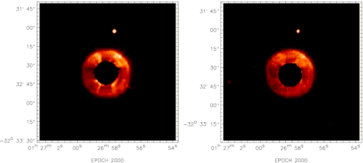
3.1 TSS images of R~Scl in the KI and Na D filters
The TSS images of R~Scl in the KI and Na D filters reveal remaining brightness distributions in the form of essentially uniform-intensity disks outside the masked areas, Fig 2. The NW regions of the disks show a somewhat enhanced emission in both filters, but there remains distortions in the images that limit the useful azimuthal information. The azimuthally averaged radial brightness profiles are relatively constant (outside the masked area) within an outer radius of 21 in both filters (corresponding to 1.11017 cm at a distance of 360 pc, see Sect. 5.2), Fig. 3. The outer radius is obtained by fitting a step function, smoothed by a seeing Gaussian, to the radial profiles, (see Sect. 3.4). The outer radius is defined as the half power radius of the fit. The outer edges of the radial brightnesses are not as sharp as the seeing smoothed step function, but the half power radii are only larger by 2 than the radii where the intensities start to drop. The emission is fainter in the Na D filter. We interpret the relative faintness in the Na D image as due to the star being fainter in this filter, and the scattering being at least partially optically thick (see Sect. 4).


In Fig. 4 we plot the estimated disk radii (in the KI and Na D filters), defined again as the half power radius of a fitted smoothed step function, as a function of position angle (PA). The brightness disks appear close to circular in both filters, with only small deviations at the 5% level. This indicates an emitting region with an overall spherical symmetry. The deviations can be partly attributed to the uncertainty in the position of the star behind the coronographic mask, but there is no clear tendency for an overestimate of the radii in a range of PAs and an underestimate in the complementary interval, as would be expected from a bad centring. Furthermore, the deviations seem to be reproduced in the same manner in both filters, suggesting actual slight departures from spherical symmetry.
Deconvolution of CO(=3–2) data, obtained with a 16 beam, using the Maximum Entropy Method shows a marginally resolved detached shell with a CO peak intensity radius which is significantly smaller, by about a factor of two, than the scattering envelope observed in the resonance line filters (Olofsson et al. olofsson96 (1996)). We will further discuss this in Sect. 5.2.
3.2 TSS images of U~Ant in the KI and Na D filters
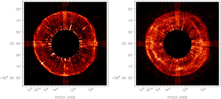
The TSS images of U~Ant in the KI and Na D filters provide spectacular results, Fig 5. In the KI filter image a geometrically thin, almost circular, ring with a diameter of 85 is centred on the star. This is most likely the result of limb brightening in a geometrically thin, essentially spherical shell. Due to the bad coronographic optics, the image contains striation and diffraction spikes that could not be removed during the reduction, and this limits the available azimuthal information.
The azimuthally-averaged radial brightness profile in the KI filter presented in Fig. 6 shows a very pronounced intensity peak, and the mean shell radius was estimated to be 43 (the corresponding linear radius is 1.71017 cm at the adopted distance of 260 pc, see Sect. 5.2) by fitting a brightness distribution appropriate for an optically thin homogeneous shell (see Sect. 3.4). This shell radius estimate from the scattered light agrees very well with the peak intensity radius of the detached CO shell observed by Olofsson et al. (olofsson96 (1996)), 41 (they have estimated their angular resolution to be 15, but the peak intensity radius has an uncertainty of only a few arc seconds). The emission tapers off gradually towards the centre, and there are indications of additional structure, which is more prominent in the Na D filter data. The emission decreases drastically beyond the peak radius, but the radial profile also shows a small bump at 50.
In the TSS image of U~Ant in the Na D filter we also clearly see the circumstellar emission, Fig. 5. However, the morphology is quite different from that obtained in the KI filter, in the sense that the brightness stays at nearly constant level much closer to the star. In fact, the appearance suggests a multiple-shell structure, which is also seen in the azimuthally averaged radial brightness profile, Fig. 7. At least two, maybe three, different components are discernible, and the two outer components may not be concentric. Fitting shell brightness distributions to these components (see Sect. 3.4), we have determined shell radii of roughly 25, 37, and 43 (1.0, 1.4, and 1.71017 cm at a distance of 260 pc), although the result for the innermost component is very uncertain. The outer component coincides with the dominant peak in the KI filter image, and the peak radius of the detached CO shell. The difference between the observations in the Na D and the KI filters can be explained in terms of optical depth effects (see Sect. 4). The possible existence of multiple shells is surprising and this will be further discussed in Sect. 5.2. As in the KI filter image, there is a small bump in the radial brightness profile at 50 offset from the star. This emission is only marginally visible in the image of the shell.


Fig. 8 shows the estimated shell radii (for the 43 shell) at different PAs in the KI and Na D filter images of U~Ant. The deviations from circular symmetry are very small, 3%. Thus, we can also infer a remarkable overall spherical symmetry for the U~Ant shell. The small deviations from the means follow the same pattern in both filters, indicating minor irregularities in the shell morphology. The KI filter image reveals edge-effects, which appear in the form of double-peaks in the radial brightness profiles, Fig. 9. We interpret this as due to small undulations in the shell structure along the line-of-sight, but a more complex origin cannot be excluded.


3.3 TSS images of U~Ant in other filters
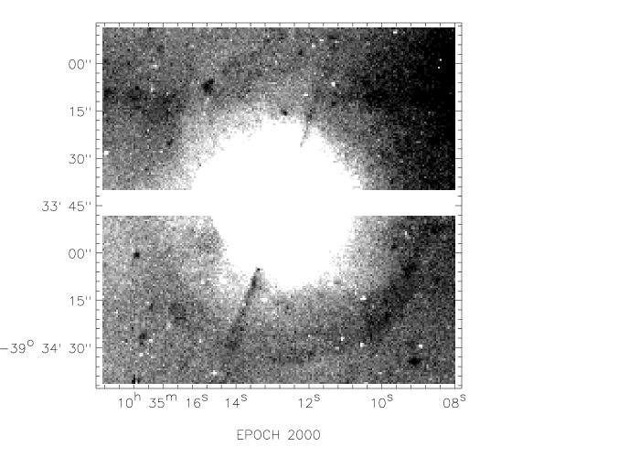
We have also made observations of U~Ant in filters containing no strong resonance lines (v, b, and Gunn z). Fig. 10 shows the TSS image of U~Ant in the b filter. We have binned the image by 22 pixels in order to increase the sensitivity to extended emission. We find that weak emission is detected, especially towards the south. The presence of a bright field star with a very long horizontal diffraction pattern makes the detection more problematic towards the north. The azimuthally averaged radial brightness profile clearly shows an emission bump extending from about 35 to 55. We have estimated its radius to be 46 by fitting a Gaussian to the radial brightness profile. This is about the same radius as those of the small outer bumps in the KI and Na D radial brightness profiles discussed above. We report also an upper limit, obtained from a short exposure, to any shell emission in the Gunn z filter.

3.4 The stellar and circumstellar fluxes
In order to analyse the circumstellar emission and the circumstellar structure it is enough to compare the relative fluxes of the circumstellar and stellar emission. Unfortunately, the use of a coronographic mask in the observations makes it difficult to obtain the stellar flux from an image. We have therefore tried to fit an extended point spread function of the type found by King (king (1971)) and Piccirillo (piccirillo (1973)) to estimate the stellar flux, but the resulting values appear too low by about two orders of magnitude. We have not identified the reason for this, but suspect that the use of a coronographic mask may be part of the problem. Therefore, an indirect method using a synthetic spectrum of R~Scl had to be used to estimate the stellar fluxes at the central wavelengths of the various filters. We adopted =5.8 and 5.5 for R~Scl and U~Ant, respectively. The variability of R~Scl and U~Ant (0.5 mag at visual wavelengths) introduces some uncertainty in the calculation, but the obtained values should be within a factor of two of the actual fluxes. The results are given in Tables 2 and 3.
|
|
The U~Ant shell fluxes (except in Gunn z) were calibrated using photometric standard stars, Sect. 2.2. In the case of R~Scl (and U~Ant in Gunn z) calibration data are lacking, and we have therefore converted from counts/s in the detector to fluxes above the atmosphere by correcting for atmospheric absorption, telescope aperture with a central obstruction, telescope reflectivity, instrument transmission, filter bandpasses and transmission, and the quantum efficiencies and gains of the CCDs. We estimate that the R~Scl shell fluxes are accurate to within a factor of five, and those of U~Ant within a factor of two.
We have determined the circumstellar fluxes by fitting adopted brightness distributions to the azimuthally averaged radial brightness profiles, in order to be able to estimate the brightnesses in the occulted regions, and also to separate the fluxes from the different components. In the case of R Scl we adopt a step function, smoothed by a seeing Gaussian, to fit the radial profiles. The outer radius is defined as the half power radius, Fig. 3. In the case of U Ant we have chosen, guided by the KI filter image, to assume optically thin scattering in homogeneous shells. This produces a generic brightness distribution with the shell radius and width, and the peak intensity as the fitting parameters. We have fitted such distributions, smoothed with a seeing Gaussian, to the three peaks (the components shell1, shell2, and shell3 in Table 3) in the Na D filter radial profile (ignoring for the moment the component outside the 43 shell). We have done the same for the KI filter radial profile, except that the radii of the two inner shells were kept the same as for the Na D filter radial brightness profile fit. The radial distribution of the outer component appears different from that of the others, and we have fitted a Gaussian distribution to the b filter radial brightness profile of U Ant (the component shell4 in Table 3). A Gaussian with the same location and width was subsequently fitted to the outer peaks in the KI and Na D data. The final fits are shown in Figs. 6, 7, and 11.
The shell surface brightnesses and fluxes obtained from the fits, and the ratio of circumstellar-to-stellar fluxes (CS/S-ratio) are given for both stars in the different filters in Tables 2 and 3. Also given are the estimated outer radii of the R Scl brightness distributions, and the radii and widths of the U Ant brightness distributions.
4 Analytical approach
We will in this section derive some analytical formulae appropriate for a simple analysis of our observational results in terms of line or dust scattering, in the optically thin regime, of central stellar light in a geometrically thin, spherical shell. Even a rough estimate shows that in our cases the stellar light dominates completely over the interstellar light, as opposed to e.g. the case of IRC+10216 which is heavily obscured and where the scattered light is of interstellar origin (Mauron & Huggins mauron99 (1999), mauron00 (2000)). Clearly, the CS/S-ratio in a given filter cannot exceed
| (1) |
where is the ratio of the average stellar flux density in the total scattering wavelength range, , and the average stellar flux density in the filter passband, (e.g., 1 in the case of resonance line scattering where strong photospheric line absorption removes photons in a wavelength range which is much narrower than the filter width).
In the cool, detached shells of AGB stars the total line scattering wavelength range is determined by the turbulent motion of the gas, i.e., we assume there is no velocity gradient across the shell. We have adopted a local velocity width of 1 km s-1, a value which is typically assumed in the analysis of CSE radio line emission (Schöier & Olofsson schoier (2001)), and which is consistent with the CO radio line data of detached shells (Olofsson et al. olofsson00 (2000)). This gives a maximum CS/S-ratio of about 210-4 and 410-4 for line scattering in the narrow KI ( only one of the doublet lines) and Na D (both doublet lines) filters, respectively (0.5 for the strong resonance lines, =5 nm). A comparison with the observed values, Tables 2 and 3, indicates that we are close to these ratios in both the KI and Na D filters for both sources (exceed them by at most a factor of four). For dust scattering the maximum CS/S-ratio is 1, since = and =1.
A more strict limit is provided by the fact that the observed surface brightness in a filter cannot exceed the source function for scattering at the position of the shell, i.e., the mean intensity of the stellar radiation and the scattered radiation in the optically thick shell. This results in
| (2) |
where is the stellar flux density at the Earth averaged over the filter passband , and is the angular size of the shell.
Using the observed shell sizes the maximum surface brightnesses for line scattering are 510-16 and 410-16 erg/s cm2 for R~Scl and 110-16 and 110-16 erg/s cm2 for U~Ant in the KI and Na D filters, respectively [from now on, in the case of U~Ant, we concentrate on the 43 shell (shell3) for which we also have information from the CO radio line observations]. The observed peak surface brightnesses are at most a factor of four above these values. The maximum surface brightnesses for dust scattering are much higher, 210-11 and 110-12 erg/s cm2 for R~Scl in the KI and Na D filters, respectively, and 710-13, 310-13 and 710-14 erg/s cm2 for U~Ant in the KI, Na D, and b filters, respectively.
We will proceed with a simple analysis of the observed scattered emission based on the assumption of optically thin scattering in a shell with no velocity gradient. The circumstellar scattered flux at the Earth, integrated over the total scattering wavelength range, in the optically thin regime is given by
| (3) |
so that the expected CS/S-ratio is given by,
| (4) |
where is the number of scatterers, is the scattering cross section, and is the shell radius [(4) is the optically thin limit of Eq.(1)]. The assumption of optically thin scattering requires that the total scattering surface is smaller than the geometrical surface, i.e.,
| (5) |
4.1 Line scattering
In the case of line scattering and assuming a Boltzmann distribution of the level populations, the number of scatterers and the cross section are given by,
| (6) |
| (7) |
where is the shell mass, is the mean molecular weight, is the partition function, is the statistical weight of the lower level, is the excitation energy of the lower level, is the number abundance of species X with respect to H, is the fraction of X that remains in neutral form, and is the oscillator strength of the line (for the other parameters we use common notations).
It is now possible to use Eqs. (4), (6), and (7) to estimate whether the observed emission in the KI and Na D filters can be attributed to line scattering. Using the shell radii obtained from the observations, assuming a shell mass of 0.01 M⊙, which is a typical value derived from CO observations (Schöier & Olofsson schoier (2001)), and a solar abundance of potassium, and assuming a local velocity width of 1 km s-1, we find that in order to reproduce the observed CS/S-ratios in the KI filter only 6% of the K atoms in R~Scl and 4% in U~Ant must remain in neutral form. The corresponding values assuming a solar abundance of sodium is 0.3% for R~Scl and 0.2% for U~Ant.
The transition between optically thin and thick line scattering can be obtained from Eqs. (5), (6), and (7). Saturation in the KI line is reached with =0.02 for R~Scl and =0.04 for U~Ant. For the Na D lines, saturation is reached already with =610-4 for R~Scl and =10-3 for U~Ant. The values of required to obtain the observed CS/S-ratios in R~Scl are higher than this by a factor of a few, and hence any KI and Na D line scattering is likely to be optically thick. In the case of U~Ant, at least partially, optically thin KI and Na D line scattering is possible. We note here that these estimates are highly uncertain, and shall only be taken as a guide for the final interpretation.
The ionization degree of the atoms in the shells is determined by stellar, as well as interstellar, UV photons. If we consider the stars to be blackbodies with a temperature of 2500 K and a luminosity of 5000 L⊙, and examine, as a first approximation, photons of 6 eV (this is in the region where the KI photoionization cross section has its maximum, and also close to the ionization energy of Na), we find stellar photon flux densities at the shell radii of about 210-5 cm-2 s-1 Hz-1 in the case of R~Scl and 10-5 cm-2 s-1 Hz-1 for U~Ant (note that this is very dependent on the assumed photon energy, and an accurate calculation requires an integration over the ionization cross section and the true stellar radiation field, which declines rapidly at these short wavelengths). Draine (draine (1978)) gives an interstellar photon flux density at 6 eV of about 210-3 cm-2 s-1 Hz-1. Therefore, ionization by interstellar UV photons clearly dominates at the present time. The atoms, however, have been exposed to a much stronger stellar radiation field in the past when they were closer to the star. The stellar and interstellar photon fluxes were comparable at a radius of 1016 cm. In other words, in R Scl and U Ant the stellar radiation dominated for about 10% and 5% of the expansion time, respectively. The ionization is counteracted by recombination, but it would lead too far in this connection to analyse this in detail (see e.g. Glassgold & Huggins glassgold (1986)). Mauron & Caux (mauron92 (1992)) have estimated that the ionization rate of KI due to the interstellar radiation field is about 510-11 s-1. This gives an expected lifetime for the neutral species of 650 yr if the interstellar radiation field dominates and there is no shielding. Taken into account that both the R~Scl and U~Ant shells are around (2–3)103 yr old, the amount of K that remains in neutral form in these shells is 0.02. This number is in reasonable agreement with the above required values of . We expect the ionization degree of Na to be comparable to that of K, and hence that the Na scattering is considerably optically thicker than the K scattering.
Thus, we find that the emission in the KI and Na D filters can, in principle, be explained by scattering in the resonance lines of those potassium and sodium atoms that remain in the detached shells. Our simple calculations also suggest that the Na D lines can produce optically thick scattering (as seems to be the case for both R~Scl and U~Ant), while KI line scattering may be at least partly optically thin towards U~Ant, and this would explain the different appearances in the U~Ant KI and Na D filter images.
4.2 Dust scattering
In the case of dust scattering, and assuming single-sized, spherical grains, we have the following relations for the number of scatterers and the scattering cross section,
| (8) |
| (9) |
where is the dust-to-gas mass ratio, is the density of a dust grain, is the grain radius, and is the grain scattering efficiency. If the condition for Rayleigh scattering is fulfilled (i.e., 0.16) we have
| (10) |
where is the complex index of refraction of the dust particle relative to the surrounding medium.
Using Eqs. (5), (8), and (9), typical values for the different parameters, (=0.005, =2 g cm-3, =0.1m, 1), and =0.01 M⊙, we find for the shells of R~Scl and U~Ant that the area-ratios are 0.02 and 0.01, respectively, i.e., any dust scattering must be optically thin. Alternatively, the circumstellar medium is highly clumped, which may indeed be the case (Olofsson et al. olofsson00 (2000)).
We can now estimate whether it is possible to fit the CS/S-ratios in the KI, Na D, and b (for U~Ant) filters assuming only dust scattering. Using Eqs. (4), (8), and (9), and the fact that =, we find that this is, in principle, possible provided that is about 4103 cm-1 and only weakly dependent on the wavelength. The latter requires 0.1m, and for such qrains 4103 cm-1. In addition, however, we have the requirement of optically thick emission for R~Scl in the KI and Na D filters and U~Ant in the Na D filter, which is obviously not consistent with the low CS/S-ratios and dust scattering, unless the circumstellar medium is highly clumped.
We also estimate whether it is possible to explain the CS/S-ratios for the component shell4, which has a very different radial distribution than the bulk emission in the KI and Na D filters, by dust scattering. This is possible if we assume a shell mass of 0.01 M⊙, =0.005, =2 g cm-3, and Rayleigh scattering, i.e., we substitute (10) in (9), with an average grain size of 0.03m and =1.6. This grain size is consistent with Rayleigh scattering also in the b filter since 0.05.
5 Discussion
5.1 The nature of the scattered light
No doubt, the circumstellar emission that we detect is due to scattering in atomic/molecular lines and/or by dust particles. We proceed now with a number of argument for and against different scattering agents.
First, we note that the observed CS/S-ratios and surface brightnesses are remarkably close to the maximum allowed values for line scattering in the KI and Na D filters, and well below those allowed by dust scattering. We believe that the uncertainties in the calibration of our data, and in some of the assumptions made (e.g., no velocity gradient, and the adopted local velocity width, shell mass, etc.), are such that a factor of a few can be accomodated with margin.
Second, Gustafsson et al. (gustafsson (1997)) have shown, using spectroscopic observations, that in the case of R~Scl there exist KI resonance line scattered emission out to at least 12 from the star, and that its brightness decreases as the third power of the angular distance from the star, i.e., they see no hint of a detached shell. However, beyond about 12 the circumstellar emission is lost in the noise; their CAT/CES observations are clearly less sensitive than our 3.6m observations due to the smaller telescope and the optical losses in the spectrometer. We find a brightness of about 210-15 erg s-1 cm-2 arcsec-2 for the circumstellar emission in the KI filter beyond 12. This is a factor of five lower than the brightness obtained by Gustafsson et al. at an offset of 10, and hence the data are not inconsistent, although there is considerable uncertainty in our measured fluxes and to a lesser extent also in the fluxes reported by Gustafsson et al..
Finally, the U~Ant images appear very different in the three filters. In particular, the difference between the KI and Na D filter images could be naturally explained as an effect of, at least partially, optically thin line scattering in the former, and essentially optically thick line scattering in the latter. Also the appearance of the R~Scl KI and Na D filter images, i.e., the uniform surface brightnesses, can only be explained by optically thick scattering, and since the observed CS/S-ratios are much less than one, this requires a highly clumped medium in the case of dust scattering.
On the other hand, the observed emission in the b filter has a very different radial distribution than those in the KI and Na D filter images, and an interpretation in terms of dust scattering appears more reasonable here. There are reasons for obtaining a positive result only in the b filter. For small particles the expected wavelength behaviour for the scattering process is such that we expect a higher contrast between the scattered and direct stellar components in a blue filter than in a red one. For observations in a filter with a much redder central wavelength than that of the b filter (e.g., Gunn z) the reduction becomes more problematic, since the star is so bright that the circumstellar emission is swamped by the photospheric light even in the presence of a coronographic mask, and the scattering efficiency is also lower. On the other hand, in a filter centred at even shorter wavelengths (e.g., v) the cool carbon stars have such a dramatic drop in their brightness (typically, B-V3) that the number of stellar photons which can be scattered decreases drastically, pushing the circumstellar emission down below the detection limit, even if the dust scattering efficiency increases further at shorter wavelengths.
Although we lack a definite proof (e.g., no spectroscopic information), we favour an interpretation where the main emission in the KI and Na D filters are due to resonance line scattering. We further argue that weak features in the KI, Na D, and in particular b, filters are due to Rayleigh scattering by small grains. Similar observations done in a filter containing no resonance lines and centred on the wavelength range between the Na D and KI lines (e.g., H) will ultimately help us discern whether the emission is due to resonance line or dust scattering. Unlike the b and Gunn z filters, the stellar flux and the dust scattering efficiency in such a filter lie in between their values at the Na D and KI wavelengths in which we have clearly detected circumstellar scattered light. Imaging through a very narrow filter which is tunable over the KI and/or Na D lines would also be an attractive observational mode. Awaiting such data, our interpretation must be regarded as only tentative.
This interpretation leads to different locations of the gas and the dust, in terms of the outer edges of shell3 and shell4 the difference is about 7 (i.e., Rdust-Rgas 31016 cm), which may at first seem surprising. However, this can be interpreted in terms of a drift of the dust particles with respect to the gas, produced by the radiation pressure on the dust grains. Using a gas shell expansion velocity of 18.1 km s-1 as derived from CO observations (Olofsson et al. olofsson96 (1996)), this drift velocity is estimated to be about ()/ 3 km s-1. This is a perfectly reasonable value for a mass loss rate approaching 10-5 M⊙ yr-1 (Kwok kwok75 (1975)), which is in the range of mass loss rate estimates for the detached CO shells (Schöier & Olofsson schoier (2001)).
5.2 The structure of the shells
The images of R Scl and U Ant obtained in circumstellar scattered light confirm the results on detached circumstellar shells obtained previously from CO radio line data, but also reveal new interesting features.
The CO data on R Scl show a marginally resolved detached shell. Modelling of the CO data, as well as HCN and CN radio line data, suggests a relatively thick shell, 12, with a mean radius of 12, i.e., an outer radius of 18 (Olofsson et al. olofsson96 (1996)). This outer radius agrees reasonably with the relatively sharp outer ‘disk’ edges at 21 in our optical images, so that the radio line emission and the scattered emission may be consistent with each other, but higher spatial resolution CO observations and more detailed modelling of the CO data are required to resolve this question. In particular, the inability to separate the emission from the present mass loss envelope and the detached shell make the modelling of the radio lines very uncertain. The high optical depths of the circumstellar scattered emission will make it difficult to obtain more information on the shell’s structure from such data, although polarization observations may help in this respect.
Additional information on the R~Scl shell is obtained from the spectroscopic KI observations of Gustafsson et al. (gustafsson (1997)). They found that their data, within 10 of the star, are consistent with a constant mass loss rate of about 510-7 M⊙ yr-1 if 100% of the potassium atoms remain neutral. This amounts to a mass of about 510-4 M⊙ inside 10, i.e., considerably lower than the estimated CO shell mass. This suggests that the shell has detached and that there is much less mass inside about 10, but the mass estimate of Gustafsson et al. can be higher if the amount of neutral potassium, for which there is presently no constraint, is lower.
Using the expansion velocity of the detached CO shell, 15.9 km s-1 (Olofsson et al. olofsson96 (1996)), and a distance of 360 pc derived from the period-luminosity relation for carbon stars (Groenewegen & Whitelock groenewegen (1996)), we estimate that the outer radius, 21, corresponds to an age of 2.3103 yr. At this time a drastic change in the mass loss properties of R Scl must have occurred over a time scale of a few hundred years, as evidenced by the sharp cut-offs in the radial profiles of the scattered light. This conclusion is also valid in an interacting wind model, where the shell represents the shock zone between a fast and a slow stellar wind, but the time estimates may have to be redone.
In the case of U Ant the CO data clearly reveal a detached shell whose radius of 41 is relatively well determined, but where the width is unresolved at 15 resolution (Olofsson et al. olofsson96 (1996)). To our surprise, the optical images, in particular the one obtained in the Na D filter, suggest a multiple-shell structure, where the shell at 43 dominates in mass, and where there is at least one inner shell, at 37. The dominant CO emission apparently comes from the 43 shell. The fit of a shell brightness distribution to this component in the KI filter radial brightness profile is not perfect, but nevertheless suggests that the shell is geometrically very thin, 3, which should be regarded as an upper limit since undulations in the shell structure, optical depth effects, and seeing will broaden the azimuthally averaged radial brightness profile. This width is comparable to those of the thin CO shells detected towards the carbon stars U Cam and TT Cyg (Lindqvist et al. lindqvist99 (1999); Olofsson et al. olofsson00 (2000)). We can also use the fit to the KI radial brightness distribution to estimate the masses of the inner shells relative to that of the outer shell. Taking into account that the number of photons per unit area to be scattered decreases as the radius squared, we find that the masses of the two inner shells are only a few percent of the mass of the outer shell. The dynamic range of the CO maps is limited, and also considering the poor spatial resolution, we can only conclude that any CO emission from the two inner shells must be at least a factor of five weaker than that of the 43 shell. Thus, the CO data do not exclude the existence of inner shells with the properties found here. The difference between the morphology of the KI and Na D filter images can be explained by resonance line scattering and higher optical depths in the Na D lines. This could also explain the poor fit of geometrically thin shell brightness distributions to the Na D data. Optical depth effects tend to broaden the profile towards the star, while leaving the outer edge essentially unchanged. It is not obvious why we see shells inside the 43 shell if the Na scattering is optically thick. Two possible explanations are a clumpy medium or differences in kinematics of the shells which will make the outer shell transparent to emission from the inner shells.
Using the CO shell expansion velocity of 18.1 km s-1 (Olofsson et al. olofsson96 (1996)), and a distance of 260 pc to U~Ant derived from the Hipparcos parallax (Alksnis et al. alksnis (1998)), the ages of the shell1, shell2, and shell3 components are estimated to be 1.7, 2.6, and 3.0103 yr. The time interval between the shells is consequently 400–900 yr. The morphology resembles to a large extent the multiple-shell structures (in the form of arcs, i.e., incomplete shells centered on the star) seen towards the extreme carbon star IRC+10216 (time interval 200–800 yr; Mauron & Huggins mauron99 (1999), mauron00 (2000)), and the post-AGB objects IRAS 17150–3224 (200–300 yr; Kwok et al. kwok (1998)), and CRL2688 (150–450 yr; Sahai et al. sahai (1998)), and similar structures towards the M supergiant Cep where shells are seen in KI emission (Mauron mauron (1997)). In these cases the shells represent density enhancements on a general density law. Suggestions for mechanisms for the formation of these shell structures range from modulated mass loss due to a companion (Harpaz et al. harpaz (1997)), shock waves in the CSE due to a close binary (Mastrodemos & Morris mastrodemos (1999)), mass loss variations due to surface effects related to a magnetic activity cycle strengthened by a binary companion (Soker soker (2000)), and pulsation induced effects internal to the star (Icke et al. icke (1992)). It is not clear whether the putative multiple-shell structure seen towards U Ant is of the same type. An attractive alternative explanation is that there exist only two shells (shell2 and shell3), of which the outer one is the shock formed by a fast, short-term wind running into a slower, long-term wind, and the inner shell is the reverse shock set up by this interaction. The shells are separated by 6 and over the lifetime of the outer shell this corresponds to a reverse velocity of about 3 km s-1, which is not unreasonable. We will await more data (e.g., obtained in polarization mode) before further speculating on this tentative multiple-shell structure and its relevance for mass loss on the AGB.
Acknowledgements.
We are grateful to the referee, M. Jura, for detailed and constructive criticism, which lead to a better presentation of the data and their interpretation. This research is partially financed by the Swedish Natural Science Research Council, and DGD has a NOT/IAC graduate study stipend.References
- (1) Alksnis A., Balklavs A., Dzervitis U., 1998, A&A 338, 209
- (2) Beckwith S., Gatley I., Persson S.E., 1978, ApJ 219, L33
- (3) Bernat A.P., Lambert D.L., 1975, ApJ 201, L153
- (4) Bujarrabal V., Cernicharo J., 1994, A&A 288, 551
- (5) Busso M., Gallino R., Wasserburg G.J., 1999, ARA&A, 37, 239
- (6) Chan S.J., Kwok S., 1990, A&A 237, 354
- (7) Draine B.T., 1978, ApJS 36, 595
- (8) Frogel J.A., Persson S.E., Cohen J., 1980, ApJ 239, 495
- (9) Glassgold A.E., 1996, ARA&A 34, 241
- (10) Glassgold A.E., Huggins P.J., 1986, ApJ 306, 605
- (11) Gustafsson B., Eriksson K., Kiselman D., Olander N, Olofsson H., 1997, A&A 318, 535
- (12) Greenhill L.J., Colomer F., Moran J.M., et al., 1995, ApJ 449, 365
- (13) Groenewegen M.A.T., Whitelock P.A., 1996, MNRAS 281, 1347
- (14) Habing H.J., 1996, A&AR 7, 97
- (15) Hamuy M., Walker A.R., Suntzeff N.B., et al., 1992, PASP 104, 533
- (16) Harpaz A., Rappaport S., Soker N., 1997, ApJ 487, 809
- (17) Hashimoto O., Izumiura H., Kester D.J.M., et al., 1998, A&A 329, 213
- (18) Iben I., 1981, in: Proc. IAU Colloq.59, Effects of Mass Loss on Stellar Evolution, ed. C. Chiosi and R. Stalio (Dordrecht:Reidel), p.373
- (19) Icke V., Frank A., Heske A., 1992, A&A 258, 341
- (20) Ivezic Z., Elitzur M., 1995, ApJ 445, 415
- (21) Izumiura H., Kester D.J.M., de Jong T., et al., 1995, Ap&SS, 224, 495
- (22) Izumiura H., Hashimoto O., Kawara K., et al., 1996, A&A 315, L221
- (23) Izumiura H., Waters L.B.F.M., de Jong T., et al., 1997, A&A 323, 449
- (24) King I.R., 1971, PASP 83, 199
- (25) Kwok S., 1975, ApJ 198, 583
- (26) Kwok S., Su K.Y.L., Hrivnak B.J., 1998, ApJ 487, 809
- (27) Lindqvist M., Lucas R., Olofsson H., et al., 1996, A&A 305, L57
- (28) Lindqvist M., Olofsson H., Lucas R., et al., 1999, A&A 351, L1
- (29) Mastrodemos N., Morris M., 1999, ApJ 523, 357
- (30) Mauron N., Caux E., 1992, A&A 265, 711
- (31) Mauron N., 1997, A&A 326, 300
- (32) Mauron N., Huggins P.J., 1999, A&A 349, 203
- (33) Mauron N., Huggins P.J., 2000, A&A 359, 715
- (34) Olofsson H., Carlström U., Eriksson K., et al., 1990, A&A 230, L13
- (35) Olofsson H., Eriksson K., Gustafsson B., et al., 1993, ApJS 87, 267
- (36) Olofsson H., 1996, Ap&SS 245, 169
- (37) Olofsson H., Bergman P., Eriksson K., et al., 1996, A&A 311, 587
- (38) Olofsson H., Bergman P., Lucas R., et al., 1998, A&A 330, L1
- (39) Olofsson H., Bergman P., Lucas R., et al., 2000, A&A 353, 583
- (40) Piccirillo J., 1973, PASP 85, 278
- (41) Plez B., Lambert D.L., 1994, ApJ 425, L101 3, PASP 85, 278
- (42) Renzini A., 1981, in: Proc. IAU Colloq.59, Effects of Mass Loss on Stellar Evolution, ed. C. Chiosi and R. Stalio (Dordrecht:Reidel), p.319
- (43) Sahai R., Trauger J.T., Watson A.M., et al., 1998, ApJ 493, 301
- (44) Schöier F.L., Olofsson H., 2001, A&A, in press
- (45) Schröder K.-P., Winters J.M., Sedlmayr E., 1999, A&A 349, 898
- (46) Soker N., 2000, ApJ 540, 436
- (47) Speck A.K., Meixner M., Knapp G.R., 2000, ApJ 545, L145
- (48) Steffen M., Schönberner D., 2000, A&A 357, 180
- (49) Waters L.B.F.M., Loup C., Kester D.J.M., et al., 1994, A&A 281, L1
- (50) Weintraub D.A., Huard T., Kastner J.H., Gatley I., 1998, ApJ 509, 728
- (51) Willems F.J., de Jong T., 1988, A&A 196, 173
- (52) Zijlstra A.A., Loup C., Waters L.B.F.M., et al., 1992, A&A 265, L5