Structure and mass of a young globular cluster in NGC 6946

Abstract

Using the Wide Field Planetary Camera 2 on board the Hubble Space Telescope, we have imaged a luminous young star cluster in the nearby spiral galaxy NGC 6946. Within a radius of 65 pc, the cluster has an absolute visual magnitude $M_{V}=-13.2$, comparable to the most luminous young ‘super-star clusters’ in the Antennae merger galaxy. $UBV$ colors indicate an age of about 15 Myr. The cluster has a compact core (core radius $\sim 1.3$ pc), surrounded by an extended envelope with a power-law luminosity profile. The outer parts of the cluster profile gradually merge with the general field, making it difficult to measure a precise half-light radius ($R_{\rm e}$), but we estimate $\mbox{$R_{\rm e}$}\sim 13$ pc. Combined with population synthesis models, the luminosity and age of the cluster imply a mass of $8.2\times 10^{5}\,\mbox{${\rm M}_{\odot}$}$ for a Salpeter IMF extending down to 0.1 ${\rm M}_{\odot}$. If the IMF is log-normal below $0.4\,\mbox{${\rm M}_{\odot}$}$ then the mass decreases to $5.5\times 10^{5}\,\mbox{${\rm M}_{\odot}$}$. Depending on model assumptions, the central density of the cluster is between $5.3\times 10^{3}\,\mbox{${\rm M}_{\odot}$}\,{\rm pc}^{-3}$ and $1.7\times 10^{4}\,\mbox{${\rm M}_{\odot}$}\,{\rm pc}^{-3}$, comparable to other high-density star forming regions. We also estimate a dynamical mass for the cluster, using high-dispersion spectra from the HIRES spectrograph on the Keck I telescope. The HIRES data indicate a velocity dispersion of $10.0\pm 2.7$ km/s and imply a total cluster mass within 65 pc of $1.7\pm 0.9\times 10^{6}\,\mbox{${\rm M}_{\odot}$}$. Comparing the dynamical mass with the mass estimates based on the photometry and population synthesis models, the mass-to-light ratio is at least as high as for a Salpeter IMF extending down to $0.1\,\mbox{${\rm M}_{\odot}$}$, although a turn-over in the IMF at $0.4\,\mbox{${\rm M}_{\odot}$}$ is still possible within the $\sim 1\sigma$ errors. The cluster will presumably remain bound, evolving into a globular cluster-like object.

1 Introduction

Ever since the presence of ultra-luminous young star clusters in certain external galaxies was first suspected, the true nature of such objects has remained somewhat controversial. It took the spatial resolution of the Hubble Space Telescope to definitively prove that the compact blue objects in starburst dwarfs like NGC 1705 and NGC 1569 (Sandage, 1978; Arp & Sandage, 1985) are indeed star clusters and not merely foreground stars (O’Connell, Gallagher & Hunter, 1994). Subsequently, similar “super-star clusters” or “young massive clusters” (hereafter YMCs) have been discovered in other starburst galaxies, notably in mergers like e.g. the “Antennae”, NGC 7252 and NGC 3256 (Whitmore et al., 1993; Whitmore & Schweizer, 1995; Zepf et al., 1999). From their luminosities and reasonable estimates of the mass-to-light ratios, YMCs appear to have masses similar to those of the old globular clusters observed around virtually all major galaxies, and there is thus growing anticipation that the study of these young clusters can provide important information about how their older counterparts formed.

One remaining challenge is to verify that YMCs contain enough low-mass stars to remain bound for a significant fraction of a Hubble time. Deep HST imaging has recently allowed the stellar population of the R136 cluster in the LMC to be probed down to about 1.35 ${\rm M}_{\odot}$ (Sirianni et al., 2000), with some evidence for a flattening of the mass function below $\sim 2$ ${\rm M}_{\odot}$. Direct observations of low-mass stars in more distant extragalatic star clusters are currently far beyond reach. Brodie et al. (1998) compared features in low-resolution spectra of YMCs in the peculiar galaxy NGC 1275 with population synthesis models and concluded that their data were best explained by models with a lack of low-mass stars. However, the integrated light of these young objects is generally dominated by A- and B- type stars and cool supergiants and conclusions about low-mass stars, based on integrated spectra and/or photometry are inevitably quite uncertain and model-dependent. A potentially better way to gain insight into the stellar mass function of unresolved star clusters is to compare dynamical mass estimates with the masses predicted by population synthesis models. Should the dynamical masses turn out to be much lower than expected, this would indicate that the clusters may lack a significant number of low-mass stars. This, in turn, would imply that such objects are not similar to old globular clusters and will not survive for anything like a Hubble time, since only stars with masses below $1\mbox{${\rm M}_{\odot}$}$ have the required long lifetimes.

Dynamical masses have, so far, been estimated only for a small number of YMCs in NGC 1569 and NGC 1705 (Ho & Filippenko, 1996a, b), in M82 (Smith & Gallagher, 2000) and the Antennae (Mengel, 2001). Sternberg (1998) concluded that the velocity dispersion and luminosity of the luminous cluster NGC 1569A are consistent with a Salpeter IMF down to 0.1 ${\rm M}_{\odot}$, while the cluster NGC 1705A may have a flatter IMF slope. The luminous cluster ’F’ in M82 appears to have a somewhat lower velocity dispersion than expected from its luminosity, favoring a top-heavy IMF (Smith & Gallagher, 2001). The $\sim 100$ Myr old cluster NGC 1866 in the Large Magellanic Cloud was studied by Fischer et al. (1992), who obtained a dynamical mass of $1.35\times 10^{5}$ ${\rm M}_{\odot}$. van den Bergh (1999) pointed out that, for the luminosity and age of NGC 1866, this mass implies a very high mass-to-light radio and large numbers of low-mass stars.

In a study of 21 nearby spiral galaxies, Larsen & Richtler (1999) found several examples of YMCs. Most of these galaxies are at distances less than about 10 Mpc and thus offer attractive targets for detailed studies of their YMC populations. A particularly interesting, very luminous young cluster was found within a peculiar bubble-shaped star forming region in the nearby face-on spiral NGC 6946. Tully (1988) lists a distance of 5.5 Mpc and more recently a mean distance of $5.9\pm 0.4$ Mpc has been estimated for the NGC 6946 group from ground-based photometry of the brightest blue stars (Karachentsev, Sharina & Huchtmeier, 2000). For the remainder of this paper we adopt the latter distance estimate. The star forming region was first noted by Hodge (1967) in a search for objects similar to Constellation III in the LMC, but was then largely forgotten. Using ground-based CCD images from the Nordic Optical Telescope, the young massive cluster and its surroundings were further discussed by Elmegreen, Efremov & Larsen (2000), who estimated a total mass of about $5\times 10^{5}\,\mbox{${\rm M}_{\odot}$}$ and an age of 15 Myr based on $UBV$ colors. The ground-based data, obtained in a seeing of about $0\farcs 7$, also provided an estimate of the half-light (effective) radius of the cluster of about 11 pc. With an apparent $V$ magnitude of about 17, it may seem surprising that such a luminous object in a nearby galaxy went relatively unnoticed until recently. This may be due to the fact that NGC 6946 is located at a low galactic latitude ($b=12\deg$), in a field rich in foreground stars. Therefore, on ground-based images taken in less than optimal seeing, the cluster is easily confused with a foreground star.

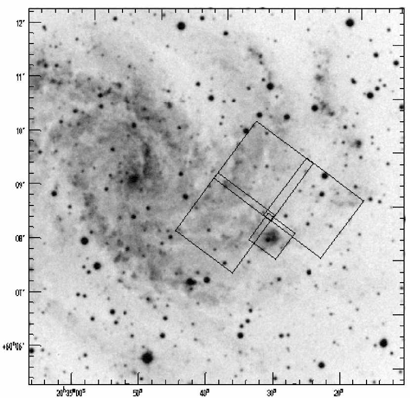
Figure 1: The WFPC2 field of view superimposed on a Digital Sky Survey image of NGC 6946. North is up and East to the left in this figure.

Here we present new HST / WFPC2 and Keck I / HIRES data for the young massive cluster in NGC 6946, labeled n6946-1447 by Larsen (1999). The WFPC2 field of view is shown in Fig. 1, superimposed on an image of NGC 6946 from the Digital Sky Survey. A color image from the Nordic Optical Telescope, showing the region around the cluster, can be found in Elmegreen, Efremov & Larsen (2000).

2 Data

2.1 HST data

WFPC2 data were acquired in Cycle 9, using the F336W ($U$), F439W $(B)$, F555W $(V)$ and F814W $(I)$ filters. The integration times were 3000 s, 2200 s, 600 s and 1400 s in the four bands, respectively, with all integrations split into two exposures in order to facilitate efficient elimination of cosmic ray hits. Initial processing (bias subtraction, flatfielding etc.) were performed “on-the-fly” by the standard pipeline processing system at STScI. The individual exposures were then combined using the IMCOMBINE task within IRAF, setting the reject option to crreject in order to eliminate cosmic ray (CR) hits.

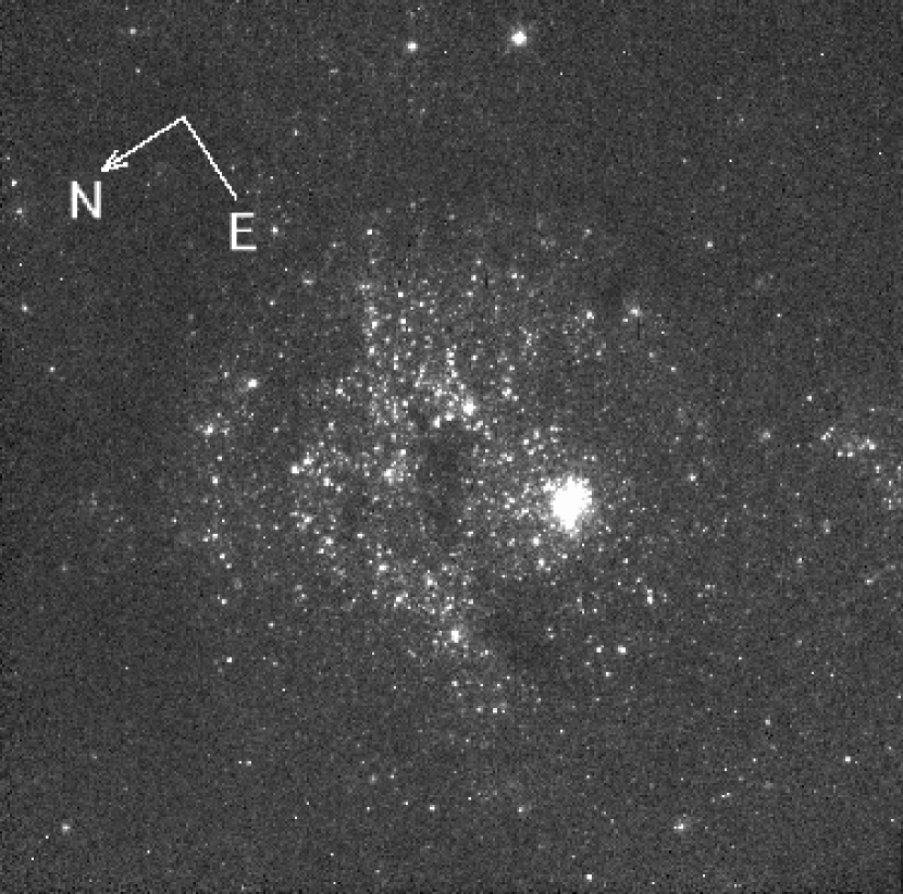
Figure 2: An F555W image showing the PC field of view. North and East are indicated by the arrow. The young globular cluster is easily recognizable as the single most luminous object, near the center of the image.

The PC field of view of the F555W exposure is shown in Fig. 2. The whole star forming complex comfortably fits on the PC chip and we do not consider data in the Wide Field chips in this paper. The YMC is easily recognizable as the single most luminous object in the field. At the distance of NGC 6946, one PC pixel corresponds to a linear scale of 1.3 pc so unless the YMC is unusually compact, its radial profile will be well resolved. In this paper we only discuss the cluster itself and its immediate neighborhood. The numerous other clusters and individual stars contained within the PC field will be discussed in a subsequent paper.

2.2 Keck data

Observations with the HIRES high-dispersion spectrograph (Vogt et al., 1994) on the Keck I telescope were obtained during two half nights in August 2000. Both nights were photometric with a seeing of around $0\farcs 9$. Following Ho & Filippenko (1996a), we used two different setups: One optical setting covering the wavelength range from 3780 Å to 6180 Å in 37 echelle orders, and a near-infrared setting ranging from 6220 Å to 8550 Å in 16 orders. For the optical setting we used the “C1” decker, providing a $7\arcsec\times 0\farcs 86$ slit, while the “D1” decker with a $14\arcsec\times 1\farcs 15$ slit was used for the near-IR setting. This provided a spectral resolution of $R=45000$ and $R=34000$ for the two settings, respectively.

The total integration times were 180 minutes and 220 minutes for the optical and near-IR spectra, split into 4 individual exposures for each setting. The slit orientation was kept constant with respect to the sky during the exposures, but was aligned with the parallactic angle at the beginning of each exposure. In addition to the cluster spectra we also obtained spectra for 11 stars of different spectral types, to be used as cross-correlation templates. These are listed in Table 1.

The reductions were performed using the highly automated “makee” package, written by Tom Barlow. “makee” automatically performs bias subtraction and flatfielding, identifies the location of the echelle orders on the images and extracts the spectra. Wavelength calibration is done using spectra of ThAr calibration lamps mounted in HIRES. Each of the individual 1-dimensional spectra were then combined using the scomb task in IRAF. In Fig. 3 we show two echelle orders from the cluster spectra compared with a G5Ia star (HR 8412) and an A7III star (HR 114). The left plot includes the $H\beta$ line. The cluster spectrum is clearly of a composite nature, showing both strong Balmer lines similar to those in early-type stars, and numerous lines due to heavier elements, as in evolved cool supergiants.

3 Results

3.1 Structure of the cluster

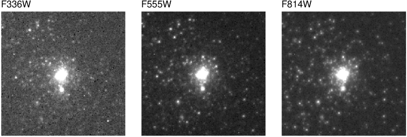
Figure 4: Close-ups of the young globular in F336W, F555W and F814W. Each image spans about 6″. Orientation is the same as in Fig. 2.

Fig. 4 shows close-ups of the cluster in F336W, F555W and F814W, each spanning 6″ or about 170 pc across. Note that another fainter cluster is located about 15 pixels (19 pc) to the North-East. In addition a number of field stars are visible, in particular in the F814W image, and also the young globular itself begins to resolve into individual stars. From Figs. 2 and 4, it is hard to tell where the cluster ends and where the general field population begins. In fact, star formation appears to have taken place over an area much larger than that directly connected with the cluster, and only the stars closest to the cluster center may actually be bound to it.

In Fig. 5 we show the integrated luminosity (left) and surface brightness (right) of the cluster as a function of radius. The photometry was done using the PHOT task within the DAOPHOT package in IRAF, measuring the background in an annulus starting at 50 pixels ($2\farcs 25$) and 50 pixels wide. The instrumental profile has not been taken into account in Fig. 5. We do not measure the luminosity profile of the cluster beyond 50 pixels, as it is clear e.g. from Fig. 2 that the irregular background at larger distances from the cluster would make such a measurement very uncertain. Nevertheless, the integrated light will probably continue to rise well beyond 50 pixels ($\sim 65$ pc). This is not unusual for young star clusters: Elson, Fall & Freeman (1987) found that young (8 – 300 Myr) clusters in the LMC are surrounded by large envelopes with power-law luminosity profiles which will probably be lost to tidal forces. Similarly, Whitmore et al. (1999) found an extended envelope with a diameter of more than 900 pc around the highly luminous “knot S” in the Antennae.

If we approximate the surface brightness $(SB)$ as a function of radius $r$ with a simple power-law of the form $SB\propto r^{\alpha}$ (for $SB$ in counts / unit area) and perform a fit to the cluster profile between $r=2$ and $r=15$ pixels, we formally obtain an exponent of $\alpha=-1.79\pm 0.03$. The fit is indicated by the dashed line in the right-hand panel of Fig. 5.

Although a power-law may provide a satisfactory fit to the outer parts of a cluster, the intensity must level off at some radius near the center. Thus, a more realistic analytic model of the cluster profile will involve some core radius $r_{c}$. Elson, Fall & Freeman (1987) found that the surface brightness profiles of young clusters in the LMC are generally well fit by analytic models of the form

$$SB\,\propto\,(1+r^{2}/r_{c}^{2})^{-\xi/2}$$ (1)

with exponent $\xi$ in the range $2.2<\xi<3.2$ and core radii from 1.3 to 7 pc. For $r\gg r_{c}$, equation (1) is similar to a power-law with slope $-\xi$, but reaches a constant value near the center.

Because the core radius of n6946-1447 is comparable to the resolution of the PC camera, it cannot be accurately estimated from a simple plot of surface brightness vs. radius. We have used a modified version of the ishape algorithm (Larsen, 1999) to fit models of the form (1) to the image of the young globular. ishape iteratively adjusts the exponent $\xi$ and the core radius $r_{c}$ and then convolves the corresponding model with the HST point-spread function (PSF) until the best match to the observed cluster image is obtained. The HST PSF is modeled using the TinyTim PSF simulator (Krist & Hook, 1997) and the modeling done by ishape also involves a convolution with the WFPC2 “diffusion kernel” (Krist & Hook, 1997). Since the diffusion kernel is best characterized for the F555W band, we used exposures in this band for the model fits.

To test the stability of the fitted parameters we carried out a number of fits, varying the fitting radius between 5 and 15 pixels and changing the initial guesses for the exponent $\xi$. The algorithm returned exponents in the range $1.98<\xi<2.18$ and FWHM values between 1.70 and 2.19 pixels. We thus adopt FWHM = $1.95\pm 0.25$ pixels and $\xi=2.1\pm 0.1$ as our estimates of the structural parameters for the cluster. Note that this is a slightly steeper profile than that obtained by a simple power-law fit to the raw cluster profile, uncorrected for instrumental effects. For the relevant range of $\xi$ values, the core radius $r_{c}=0.5\times\mbox{FWHM}$ to within 5%, i.e. $r_{c}=1.26\pm 0.16$ pc for a distance of 5.9 Mpc. This is comparable to the most compact young LMC clusters and is also a typical value for Milky Way globular clusters (Peterson & King, 1975; Harris, 1996). In 5 of the 6 fits we performed, ishape returned minor/major axis ratios between 0.91 and 0.93, while one fit (for $r=5$ pixels) returned an axis ratio of 0.97. The cluster thus seems to be somewhat elongated with an axis ratio of about 0.92, with a likely uncertainty of a few times 0.01.

Integrating equation (1) from $r=0$ to $r=\infty$, the total luminosity diverges for $\xi<2$. With our estimate of $\xi=2.1\pm 0.1$, the half-light radius ($R_{\rm e}$) is therefore not very well-defined. For $\xi=2$, (1) is identical to a King (1962) profile with infinite tidal radius. We also attempted to fit King models to the cluster profile, varying the concentration parameter, but such fits are highly sensitive to inaccuracies in the background level and turned out to be too uncertain. If we (somewhat arbitrarily) define the “total” luminosity as the luminosity contained within 50 pixels, Fig. 5 suggests $\mbox{$R_{\rm e}$}\sim 10$ pixels or about 13 pc. This crude estimate is significantly larger than the typical half-light radius for stellar clusters, but agrees well with the ground-based estimate of $\mbox{$R_{\rm e}$}\sim 11$ pc obtained by Elmegreen, Efremov & Larsen (2000). Old globular clusters typically have $\mbox{$R_{\rm e}$}\sim 3$ pc (e.g. Harris, 1996), while young massive clusters in starburst / merger galaxies such as the Antennae may have slightly larger effective radii ($\mbox{$R_{\rm e}$}\sim 4$ pc, Whitmore et al., 1999). However, because of the youth of the cluster in NGC 6946, it is quite likely that much of the loosely bound outer parts may eventually be stripped. Assuming that the core remains relatively unaffected by tidal stripping, we can calculate the half-light radius for King models with various tidal radii ($r_{t}$). Integration of the King profiles shows that the effective radius $R_{\rm e}$ and core radius are related as $\mbox{$R_{\rm e}$}=2.9\,r_{c}$ for $r_{t}/r_{c}=30$ and $\mbox{$R_{\rm e}$}=5.1\,r_{c}$ for $r_{t}/r_{c}=100$. Assuming $r_{c}=1.3$ pc for n6946-1447, we then obtain $\mbox{$R_{\rm e}$}=3.8$ pc and $\mbox{$R_{\rm e}$}=6.6$ pc for $r_{t}/r_{c}=30$ and $r_{t}/r_{c}=100$, respectively. These numbers suggest that, if the cluster evolves towards a King profile with a finite tidal radius, its effective radius could decrease significantly.

It is also worth noting that some old globular clusters have significantly larger half-light radii than 3 pc. The Harris (1996) catalog lists $R_{\rm e}$ values up to about 20 pc for some of the outer Palomar-type halo clusters, and Harris, Poole & Harris (1998) obtained a half-mass radius of about 7 pc for a globular cluster in NGC 5128, corresponding to $\mbox{$R_{\rm e}$}\sim 5.3$ pc.

3.2 Integrated photometry

In Table 2 we list photometry for the young cluster in 5 different apertures between $r=5$ pixels ($0\farcs 23$) and $r=50$ pixels ($2\farcs 25$). Again, the photometry was obtained using the PHOT task within IRAF, measuring the background between 50 and 100 pixels from the cluster center. Instrumental magnitudes measured on the PC images were transformed to the standard $UBVI$ system using the transformations in Holtzman et al. (1995). For comparison, we also list the ground-based photometry from Larsen (1999). The magnitudes and colors in Table 2 have not been corrected for galactic foreground extinction, and no aperture corrections have been applied to the HST data other than the $-0.1$ mag correction which is implicit in the Holtzman et al. calibration. Strictly speaking, the Holtzman et al. calibration is only valid for a point source observed through a $0\farcs 5$ aperture (11 pixels). In order to get the “true” magnitude for the cluster, we would have to observe it through an aperture known to encompass 90% of the total luminosity. Comparing with Fig. 5, it is quite likely that not even our $r=50$ pixels aperture contains 90% of the cluster light, so the true total magnitude of the cluster may be even brighter than $V=16.7$.

Both Fig. 5 and Table 2 show that the colors are somewhat bluer when measured through the larger apertures. To test if this could be due to wavelength-dependent aperture corrections, we convolved TinyTim PSFs in different bands with a cluster model of the form (1) and carried out photometry in the same apertures as those listed in Table 2. Two sets of tests were performed, one with the sky background kept at a fixed level of 0 and another where the background was measured on the synthetic images in the same annulus as for the real photometry. For U B and B V, we found no change larger than $\sim 0.01$ mag in the color index aperture corrections from 5 to 50 pixels, while the tests show that the $V\!-\!I$ colors are about 0.03 mag too blue when measured through the $r=5$ pixels aperture. These results are essentially independent of how the background was measured. The color gradient thus appears to be real, although it is not clear whether it is intrinsic to the cluster or due to differential reddening, contamination by field stars with different ages, or other causes.

Correcting the $r=50$ pixels photometry for a Galactic foreground extinction of $A_{B}=1.48$ (Schlegel et al., 1998) and using the reddening law by Cardelli, Clayton & Mathis (1989), we get $(\ub)_{0}=-0.75$ and $(\bv)_{0}=0.04$. Adopting the Girardi et al. (1995) ‘S-sequence’ calibration for age as a function of $UBV$ colors, this implies a cluster age of about 15 Myr, identical to the value reported by Elmegreen, Efremov & Larsen (2000) based on ground-based photometry. Our 15 Myr age estimate is also compatible with a spectroscopic age determination, based on Balmer line equivalent widths measured on low-dispersion spectra from the 6 m Special Astrophysical Observatory (SAO) telescope (Efremov et al., in preparation). Furthermore, the SAO data (as well as the Keck/HIRES spectra) show no H$\alpha$ emission from the cluster itself, indicating a lower bound on the age of $\sim 10$ Myr. Girardi et al. (1995) quote an rms scatter of 0.137 in log(age) for the S-sequence calibration, corresponding to an uncertainty of about $\pm 5$ Myr for a 15 Myr old cluster. We note that, since the S-sequence age calibration is based on LMC clusters, it may not be strictly valid for clusters with different metallicity. However, $UBV$ colors are not very sensitive to metallicity below $\sim 500\times 10^{6}$ yr so this should not lead to any large errors in the age estimate.

3.3 Velocity dispersion

From the virial theorem, the total mass ($M$), velocity dispersion ($v$) and half-mass radius ($r_{h}$) of an isolated cluster with isotropic velocity distribution are related as

$$M=a\frac{v^{2}r_{h}}{G},$$ (2)

where the constant $a$ has a value of about 2.5 (Spitzer, 1987, p. 11). Note that $v$ is the 3-dimensional velocity dispersion. What we actually measure is the line-of-sight velocity dispersion, $v_{x}^{2}=\frac{1}{3}v^{2}$.

The spectral resolution $R\sim 40000$ of the HIRES spectra is of the same order of magnitude as the expected velocity dispersion within the cluster, so simply measuring the width of the spectral lines directly on the spectra would not provide a realistic estimate of the true velocity dispersion. Instead, we follow the same procedure used by Ho & Filippenko (1996a, b). First, the cluster spectrum is cross-correlated with the spectra of a number of suitable template stars, using the fxcor task in IRAF. The velocity dispersion $v_{x}$ is then obtained from the full width at half maximum of the cross-correlation peaks, FWHM_cc. The relation between FWHM_cc and $v_{x}$ is established empirically by artificially broadening the template star spectra by convolution with Gaussian profiles and then cross-correlating the broadened template spectra with the spectra of other template stars. FWHM_cc is independent of image noise, although the height of the peak does depend on the signal/noise of the cross-correlated spectra. For very poor S/N spectra the cross-correlation peak vanishes into the noise. Our cluster spectra typically have a S/N of about 50, but by artificially adding noise to our spectra we found that consistent measurements of FWHM_cc were still possible even if the S/N of the cluster spectra was degraded to below 10.

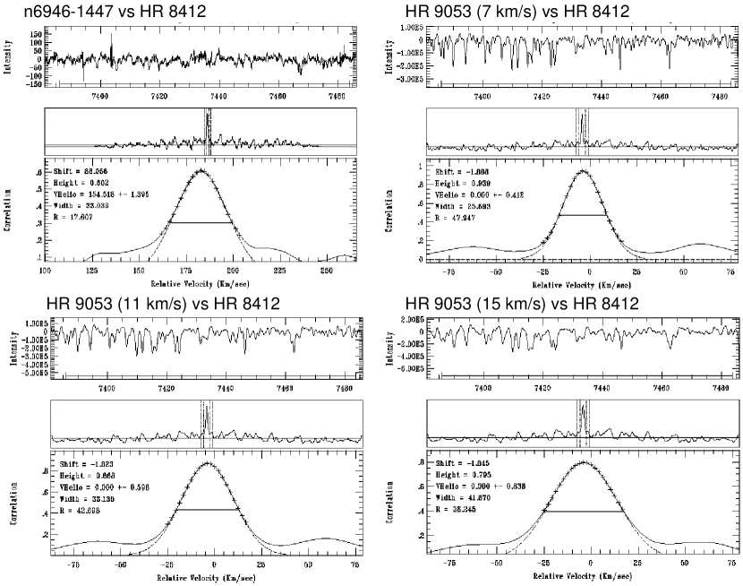
Figure 6: Cross-correlation functions for the young cluster vs. HR 8412 (upper left) and HR 9053 vs. HR 8412 where the HR 9053 spectrum has been convolved with Gaussians corresponding to velocity dispersions of 7 km/s, 11 km/s and 15 km/s.

The principle is illustrated in Fig. 6: The upper left-hand panel shows the cross-correlation peak for one echelle order of the cluster spectrum vs. the template star HR 8412. The remaining panels show cross-correlation peaks for the template star HR 9053, convolved with Gaussians corresponding to $v_{x}=7$ km/s, $v_{x}=11$ km/s and $v_{x}=15$ km/s vs. the same template star as for the cluster spectrum. For the cluster vs. HR 8412 peak, FWHM_cc = 33 pixels, compared to FWHM_cc = 25.7, 33.1 and 41.9 pixels for the three test cases. In this case, the data imply a velocity dispersion for the cluster spectrum close to 11 km/s.

In practice, we convolved the template star spectra with a number of Gaussians, having dispersions between 2 and 8 pixels (4.15 km/s to 16.6 km/s). In this way, FWHM_cc was empirically established as a function of $v_{x}$ for each combination of template stars. In Fig. 7 this is illustrated for just one combination of template stars, HR 8412 and HR 9053 (as in Fig. 6). The diamonds show FWHM_cc for the HV 9053 spectrum convolved with Gaussians of different velocity dispersions. Measurements where FWHM_cc for the cluster vs. template star peak fell outside the range corresponding to a velocity dispersion in the 4.15 – 16.6 km/s interval were rejected.

As is evident from Fig. 3, the saturated nature of the Balmer lines, along with the rapid rotation of hot early-type stars, makes them unsuitable for measurement of velocity dispersion. We therefore used regions of the spectra dominated by features from cool supergiants. Cool supergiants in a $\sim 15$ Myr old cluster are expected to be of luminosity class Ia – Ib, but to test the sensitivity of the results to the luminosity class of the templates, we observed a number of template stars covering a range of spectral types as well as luminosity classes. The template stars are listed in Table 1.

In spite of the large number of echelle orders, only relatively few turned out to be useful. In the optical setting, signal-to-noise was quite low at the blue end and only 3 orders were used. In the near-infrared setting, many orders were dominated by skylines, reducing the number of useful orders to 6. Even so, the number of individual “measurements” of the cluster velocity dispersion is very large, each “measurement” consisting of cross-correlation of a cluster spectrum with a template star and comparing with the template star cross-correlated with another smoothed template star spectrum. The distribution of all velocity dispersion measurements is shown in Fig. 8, and Table 3 lists the median velocity dispersion for each echelle order for stars of luminosity classes I, II and III separately. In some cases, only part of an order was used, as indicated by column 2 of Table 3. As can be seen from Fig. 8, the lower and upper velocity dispersion limits bracket the relevant range quite well. The median value is 10.1 km/s and the standard deviation is 2.7 km/s.

The velocity dispersions are generally larger when using template stars of luminosity class III. This is not surprising, considering the significant amounts of macro-turbulence in the atmospheres of cool supergiants which contributes to line broadening (Gray & Toner, 1987). Thus, when using normal cool giants as templates, the velocity dispersion of the cluster stars will be overestimated.

Using only template stars of luminosity class I, the median value for the velocity decreases slightly to 10.0 km/s, while the scatter remains at 2.7 km/s. As a further check, we also computed the velocity dispersion using the three best-fitting templates. As determined from the height of the cross-correlation peaks, these are HR 1009 (M0II), HR 861 (K3Ib) and HR 8726 (K5Ib). The best fits were obtained from orders 10 and 14 in the IR setting, leading to an average velocity dispersion of 9.4 km/s with a standard deviation of 0.57 km/s for this best-fitting template subsample. This value is slightly lower than that based on the full sample, but within the error margins there is good agreement. We thus adopt $v_{x}=10.0\pm 2.7$ km/s as our final estimate of the velocity dispersion of n6946-1447, noting that the uncertainty estimate is probably quite conservative.

3.4 Cluster mass

3.4.1 Dynamical mass

With an estimate of the cluster velocity dispersion and physical size at hand, we are now ready to estimate the dynamical mass. Note that the cluster radius used in equation (2) is the 3-dimensional half-mass radius $r_{h}$, which is larger than the 2-dimensional half-light or effective radius $R_{\rm e}$ measured on the images by approximately a factor of 1.3 (Spitzer, 1987). As discussed in Sect. 3.1, the effective radius of the cluster is not very well determined, but if we tentatively adopt $r_{h}=17$ pc and insert this number, together with a velocity dispersion of $v_{x}=10.0\pm 2.7$ km/s in equation (2), then the total virial cluster mass becomes $3.0\pm 1.6\times 10^{6}\,\mbox{${\rm M}_{\odot}$}$.

However, obtaining the dynamical cluster mass directly from equation (2) is inaccurate for a number of reasons: As already mentioned, the half-mass radius is uncertain because we only observe the cluster profile out to 50 pixels. As noted in Sect. 3.1, the cluster may not even have a well-defined half-light radius. Secondly, equation (2) gives the total virial mass out to some large radius, so comparing this dynamical mass with the luminosity within a radius of, say, 50 pixels may not give a realistic picture of the extent to which the luminous and dynamical masses agree. We therefore decided to perform a more detailed modeling of the cluster’s structure, as described in the following:

First, we modeled the cluster density distribution using the projected, azimuthally-averaged intensity profile in each passband, measured out to 50 pixels. We interpolated through the intensity bump from the companion cluster in the northeast using a power law fit to the profile on either side of it. The corrected profile was then assumed to come from a spherical cluster with a three-dimensional density profile, $\rho(r)$, plus some unknown light contamination from foreground and background stars. In addition to the background subtraction done prior to photometric analysis, various levels of background light were uniformly subtracted from the profile to give a range of density solutions, ranging from the background level measured at the 50th pixel down to zero background subtraction. With the largest of these subtracted backgrounds, the pure-cluster intensity went to zero at the 50th pixel, as if the cluster had an edge there.

The 3D density profile $\rho(r)$ was then determined from this projected profile by assuming that the cluster was made from a superposition of equal-density onion-skin shells, one at each pixel. In fact, the pixels of the measurements were interpolated linearly onto a finer grid with four times as many pixels, to get a better accuracy in the final density. The line-of-sight depth through each of these interpolated shells is known from the spherical symmetry assumption, so we began at the outer pixel where the intensity came only from the outer shell and obtained the density there. This outer density was determined from the ratio of the intensity to the line-of-sight depth of the outer shell. The density in the next-inner shell was determined by first subtracting the intensity at this position coming from the outer shell, using the appropriate line of sight depth and density there, from the observed intensity, and then dividing this difference by the line of sight depth through the next-inner shell. In this way, we could work from the outside to the inside and determine the 3D density of each shell. The result is the 3D density profile inside the cluster.

Figure 9 shows the fitted 3D density profile of the cluster determined from the $V$-band projected intensity profile using a background subtraction that was tuned to give the densities at the largest few radii a smooth continuation. This will be called the best-fit solution. Larger subtractions caused the density profile to drop suddenly at the 50 pixel edge, and smaller subtractions caused it to turn up. The dashed line in Figure 9 is a solution to the density structure of an isothermal cluster using the same velocity dispersion as the average determined from the observations. The straight dashed line has a slope of 2, which is the expected slope for an isothermal cluster at large radius.

The fitted 3D density profile was used in the equation of hydrostatic equilibrium in order to determine the one-dimensional velocity dispersion, $v_{1}(r)$, in each shell. This dispersion satisfies the equation

$$d\rho v_{1}^{2}/dr=-\rho GM/r^{2},$$ (3)

for mass as a function of radius, $M(r)$, obtained from the density solution, $M(r)=\int_{0}^{r}4\pi r^{2}\rho(r)dr$. To solve (3), we need to know the velocity dispersion at the edge of the cluster to give the boundary condition on pressure there. We assumed two cases: zero dispersion at the edge, corresponding to zero pressure, and a dispersion equal to the average in the cluster, determined from the fitted $\left(M/R\right)^{1/2}$ at the cluster edge, as given by the density profile. The run of dispersion, $v_{1}(r)$ was determined by integrating from the outside in. Once this dispersion solution was obtained, the square of the dispersion was averaged with a weighting proportional to the shell mass. The square root of this weighted average then gives the rms dispersion in the whole cluster, as would be observed with a slit spectrograph that covers it all. This final dispersion makes the reasonable assumption that the flux-weighted sum of Gaussian line profiles from sub-components of a total cluster is approximately equal to a Gaussian line profile itself, and that the dispersion of this summed profile is equal to the weighted quadratic sum of the dispersions of the components.

The absolute calibration for the density and mass now comes from the ratio of the observed, $v_{x}$, to the modeled, $v_{1}$, one-dimensional velocity dispersions. The absolute mass is $(v_{x}/v_{1})^{2}\times\left(1.3\;{\rm pc}\right)/G$ multiplied by the program fitted mass, which is in units of photon counts. The absolute density is $(v_{x}/v_{1})^{2}/\left(1.3\;{\rm pc}\right)^{2}/G$ multiplied by the program fitted density. Here, 1.3 pc is one pixel. For the best-fit density solution with an edge dispersion equal to the average, the mass out to the 50 pixel=65 pc radius becomes $1.67\times 10^{6}$ M_⊙, and the central density is $5.3\times 10^{3}$ M_⊙ pc^-3. With no background subtraction and an average edge dispersion, the peripheral density is greater and the central density smaller, $3.8\times 10^{3}$ M_⊙ pc^-3, to give the same observed velocity dispersion, but the mass inside 50 pixels is about the same.

The case with zero velocity dispersion at the edge is not physical but it is interesting to compare with the results given by equation 2, which is for an isolated cluster with zero pressure at the boundary. Our masses for this zero-dispersion case were systematically larger than the masses for the average-dispersion cases, particularly for the models in which there was no background subtraction. Compared to the best-fit mass above of $1.67\times 10^{6}$ M_⊙, the zero edge-dispersion masses were $1.78\times 10^{6}$ M_⊙ and $2.81\times 10^{6}$ M_⊙ for the best-fit and no-background subtraction density fits, respectively. The reason why equation 2 gives a larger mass is that it effectively includes all of the mass out to some zero-pressure boundary, even if it is beyond 50 pixels, but the 3D fit includes only the mass inside 50 pixels. Also, equation 2 assumes that the cluster has a well-defined half-mass radius while our 3D fit derives the mass directly from the luminosity profile.

In summary, the $V$-band radial intensity profile was converted to a 3D density profile using a reasonable assumption involving the level of background contamination, and this density profile was used to find a velocity dispersion profile assuming hydrostatic equilibrium with a dispersion at the edge equal to the average obtained from the density fit. The weighted average of this dispersion was then compared with the observed dispersion to give the absolute calibration for mass and density. The result is a cluster mass inside the 65 pc radius equal to $\sim 1.7\times 10^{6}$ M_⊙ and a central cluster density of $\sim 5.3\times 10^{3}$ M_⊙ pc^-3. A similar procedure was applied to the other passbands with the result that the fitted mass increases slightly with wavelength.

The fit to the velocity dispersion profile gives a result that decreases with radius by a factor of 0.6 and 0.8 from the center to the mid-radial points for the best-fit and no-background subtraction solutions, respectively. This decrease is also evident from the difference in Figure 9 between the fitted 3D density profile and the isothermal profile, considering that a steeper profile implies a smaller local scale height and a smaller dispersion for comparable acceleration. Thus we predict that the dispersion in the center of the NGC 6946 cluster is slightly higher than the dispersion at 10 to 20 pc radius. Our solution at larger radii becomes uncertain because of the unknown starlight background and the unknown outer boundary condition for the velocity dispersion.

3.4.2 Luminous mass

The dynamical mass estimate of $\sim 1.7\times 10^{6}$ M_⊙ may be compared to a photometric estimate, based on the luminosity of the cluster and a M/L ratio from population synthesis models. Such a comparison can potentially provide constraints on the stellar IMF of the cluster. For the following discussion we adopt a cluster age of $15\pm 5$ Myr, as derived in Sect. 3.2 and in Elmegreen, Efremov & Larsen (2000). Using the $V$ magnitude measured through the $r=50$ pixels aperture and correcting for a galactic foreground extinction of $A_{B}=1.48$ mag, the absolute cluster luminosity is $M_{V}=-13.2$ for a distance modulus of 28.9. This also includes a correction of $+0.1$ mag to the magnitude listed in Table 2 to account for the fact that an aperture correction of $-0.1$ mag from $r=0\farcs 5$ to $r=\infty$ is implicit in the Holtzman et al. calibration, while our measurement has already been performed through a large aperture. Thus, $M_{V}=-13.2$ represents the luminosity of the cluster out to $r=50$ pixels (65 pc), which is what should be compared to the dynamical mass derived in Sect. 3.4.1.

Using 1996 versions of the Bruzual & Charlot population synthesis models (from Leitherer et al., 1996), we can estimate the expected luminosity per unit mass for a given cluster age and stellar initial mass function (IMF). The Bruzual & Charlot models are computed for a Salpeter (1955) and a Scalo (1986) IMF, the latter approximated as a composite of 6 power-law segments. Both extend from 0.1 ${\rm M}_{\odot}$ to 125 ${\rm M}_{\odot}$, but the Scalo IMF has a steeper slope than the Salpeter IMF over most of the mass range, resulting in a higher mass-to-light ratio. For an age of $15\pm 5$ Myr, the models predict $M_{V}(1\,\mbox{${\rm M}_{\odot}$})=2.36\pm 0.3$ for the Scalo IMF and $M_{V}(1\,\mbox{${\rm M}_{\odot}$})=1.58\pm 0.4$ for the Salpeter IMF, respectively. This corresponds to a total mass of $1.68\pm 0.46\times 10^{6}\mbox{${\rm M}_{\odot}$}$ for the Scalo IMF and $0.82\pm 0.30\times 10^{6}\mbox{${\rm M}_{\odot}$}$ for a Salpeter IMF. These numbers agree fairly well with the dynamical mass within $r=50$ pixels of $1.7\pm 0.9\times 10^{6}\,\mbox{${\rm M}_{\odot}$}$ (Sect. 3.4.1), although a somewhat steeper than Salpeter IMF is preferred.

Alternatively, we may consider an IMF of the form

$$dN=\left(1-e^{-(M/M_{0})^{2}}\right)M^{-\gamma-1}dM$$ (4)

with $M_{0}=0.4\,\mbox{${\rm M}_{\odot}$}$. For $\gamma=1.35$ it approaches a Salpeter function at high masses, but has a shallower slope for $M<M_{0}$, making it similar to the IMF reported for old globular clusters by Paresce & de Marchi (2000). If the function is normalized to the pure-Salpeter function at high mass to give the same cluster luminosity, then it has only 0.67 times as much mass as the Salpeter-only function down to $0.1\,\mbox{${\rm M}_{\odot}$}$, or $0.55\pm 0.20\times 10^{6}$ ${\rm M}_{\odot}$. This is somewhat lower than the dynamical mass estimate, although an IMF of the form (4) is still within the $\sim 1\sigma$ error margins.

Although we have corrected for galactic foreground extinction, some extinction may still be present within NGC 6946 itself. Elmegreen, Efremov & Larsen (2000) suggested that the extinction may vary substantially across the star forming region surrounding the young globular. In Fig. 10 we show a $\bv,\ub$ two-color diagram with the Girardi et al. (1995) S-sequence and a cross indicating the cluster colors corrected for foreground extinction. The S-sequence is basically a fit to the colors of LMC clusters. The young globular in NGC 6946 lies almost perfectly on the S-sequence, but the reddening vector is nearly parallel to the S-sequence at this location and the cluster could be considerably younger if additional absorption is present. Furthermore, around $10^{7}$ years, cluster colors do not really change as smoothly with age as indicated by the S-sequence and ages derived on the basis of $UBV$ colors should only be taken as approximate (Girardi et al., 1995). Assuming an additional $A_{B}=0.5$ within NGC 6946, the cluster colors would correspond to an age of only $\sim 5\times 10^{6}$ yr (according to the Girardi et al. (1995) calibration) and the $V$-band luminosity per unit mass predicted by the Bruzual & Charlot models would increase by $\sim 1.1$ mag (for Salpeter IMF). Although a correction for additional reddening would also make the absolute magnitude 0.4 mag brighter in $V$, this is not enough to account for the decrease in mass-to-light ratio due to lower age. If the cluster is subject to additional reddening in NGC 6946, the net result would therefore be a decrease in the photometric cluster mass estimate, while the dynamical mass would remain unaffected as long as the relative radial profile is the same.

An additional uncertainty comes from the distance to NGC 6946. Although Karachentsev, Sharina & Huchtmeier (2000) list a mean distance modulus of 28.9 for the NGC 6946 group and adopt this as the distance of NGC 6946 itself, they actually obtain a distance modulus of 29.15 for NGC 6946. This would increase our estimate of the half-mass radius of the cluster to 20 pc and the dynamical mass from equation 2 to $3.5\pm 1.9\times 10^{6}\mbox{${\rm M}_{\odot}$}$. The fitted mass from the 3D density profile would increase by the same linear factor and become $2.7\times 10^{6}\mbox{${\rm M}_{\odot}$}$. Also at this distance, the absolute $V$ magnitude would be $-13.6$ and the resulting photometric mass $2.0\times 10^{6}\mbox{${\rm M}_{\odot}$}$ or $1.0\times 10^{6}\mbox{${\rm M}_{\odot}$}$ for Scalo or Salpeter IMFs.

In conclusion, our data are compatible with any of the three stellar IMFs considered here, although a somewhat steeper IMF than Salpeter is preferred. An IMF with Salpeter slope down to $\sim 0.4\,\mbox{${\rm M}_{\odot}$}$ and a log-normal shape below this limit is still within the error limits, but it is clear that our data do not favor a top-heavy IMF with any significant lack of low-mass stars.

3.5 Central density

The central density $\rho_{0}$ of the cluster can be estimated from the central $V$-band surface brightness $\sigma_{0}(V)$ in mag arcsec^-2, mass-to-light ratio $M/L$ and core radius in pc (Peterson & King, 1975; Williams & Bahcall, 1979):

$$\rho_{0}=\frac{3.44\times 10^{10}}{Pr_{c}}10^{-0.4\sigma_{0}(V)}(M/L)\,\mbox{${\rm M}_{\odot}$}\,\mbox{pc}^{-3}$$ (5)

where $P\approx 2$. Assuming a light profile of the form (1) with $\xi=2.1$ and an extinction-corrected $V$-band magnitude of 16.0 within 20 pixels (Table 2), the central surface brightness is $\sigma_{0}(V)=12.3$ mag arcsec^-2. Here we have used the $r=20$ pixels aperture for reference in order to avoid extrapolation of the model profile to larger radii. Measuring the light directly on the image gives $\sigma_{0}(V)=13.2$ mag arcsec^-2 within the central $r=0.5$ pixels. The direct measurement is expected to underestimate the central surface brightness because the central cusp of the profile is smeared by the finite resolution of the PC. For the same reason, the estimate of $\rho_{0}=5.3\times 10^{3}\,\mbox{${\rm M}_{\odot}$}\,{\rm pc}^{-3}$ for the central density from Sect. 3.4.1 is also likely to be an underestimate. In the following we adopt $\sigma_{0}(V)=12.3$ mag arcsec^-2 as our best estimate of the central surface brightness.

For a mass of $(1.7\pm 0.9)\times 10^{6}\,\mbox{${\rm M}_{\odot}$}$ and absolute $V$ magnitude $M_{V}=-13.2$, the mass-to-light ratio is $M/L=0.11\pm 0.06$. Inserting in equation (5), the central density is then $\rho_{0}=(1.7\pm 0.9)\times 10^{4}\,\mbox{${\rm M}_{\odot}$}\,{\rm pc}^{-3}$. We can also use the population synthesis models instead of the dynamical mass to derive $M/L$ ratios. For an IMF of the form (4) with $M_{0}=0.4$ and $\gamma=1.35$, we get a $M/L$ ratio of 0.039 and $\rho_{0}=6.2\times 10^{3}\,\mbox{${\rm M}_{\odot}$}\,{\rm pc}^{-3}$, which may be considered a lower limit. In any case, the central density is on the order of $10^{4}\,\mbox{${\rm M}_{\odot}$}\,{\rm pc}^{-3}$ and thus similar to that of the densest stellar clusters in the Milky Way, such as Monoceros R2 and the Trapezium cluster (Carpenter et al., 1997; Prosser et al., 1994) and to the R136 cluster at the center of the 30 Dor complex in the LMC (Campbell et al., 1992), but the total number of stars and physical dimensions of n6946-1447 are much larger.

4 Discussion

With a total mass somewhere around $10^{6}\,\mbox{${\rm M}_{\odot}$}$, n6946-1447 is about an order of magnitude more massive than the most massive young cluster in the LMC, NGC 1866 (Fischer et al., 1992) and many orders of magnitude more massive than typical open clusters in the Milky Way. It is, however, comparable to the most massive clusters in merger and starburst galaxies such as the Antennae (Zhang & Fall, 1999). This clearly illustrates that, although such clusters are mostly observed in merger galaxies and other starburst environments, they can also form far from the nucleus in quite normal, apparently undisturbed disk galaxies. Violent interactions such as galaxy collisions may help to create an environment that is favorable for formation of massive clusters, but such events are evidently not a necessary condition. The density near the cluster center seems to be similar to dense star forming regions in the Milky Way. Thus, the basic star forming mechanism at work may well be the same, although proceeding at a much larger scale in n6946-1447.

It is also of interest to compare n6946-1447 with two of the most luminous old globular clusters in the Milky Way, $\omega$ Cen and 47 Tuc. From their dynamical properties, Meylan & Mayor (1986) estimate total masses for the two clusters of $2.9\times 10^{6}\,\mbox{${\rm M}_{\odot}$}$ and $1.3\times 10^{6}\,\mbox{${\rm M}_{\odot}$}$, respectively. Considering that a significant fraction of the mass may be located beyond 65 pc, this makes n6946-1447 comparable in mass to these two old globular clusters. 47 Tuc has a relatively compact core with $r_{c}=0.46$ pc, while $\omega$ Cen is a quite loosely structured cluster with $r_{c}=3.8$ pc (Harris, 1996). The effective radii of the two clusters are 3.5 pc and 6.2 pc. Our estimate of the core radius for n6946-1447 of 1.3 pc is intermediate between 47 Tuc and $\omega$ Cen, while the effective radius is larger than for either of the two old globulars. As argued in Sect. 3.1, the outer parts of the cluster may eventually be stripped away and this might decrease the effective radius of n6946-1447 over time. The rotation curve of NGC 6946 indicates a mass of $\sim 3\times 10^{10}\,\mbox{${\rm M}_{\odot}$}$ within the location of n6946-1447 at about 4.5 kpc from the center (Carignan et al., 1990). For a cluster mass of $1\times 10^{6}\,\mbox{${\rm M}_{\odot}$}$, this corresponds to a tidal radius of about 70–100 pc (King, 1962; Keenan, 1981). This number depends only weakly on the exact masses of the galaxy and cluster, but assumes a homogeneous gravitational field. In practice, passages near giant molecular clouds, through spiral arms etc. may further contribute to stripping of stars from the cluster.

One outstanding question has been whether or not young massive clusters will be able to survive for any considerable amount of time. Here we find that the dynamical mass estimate of n6946-1447 agrees well with to the mass predicted by various population synthesis models. Formally, a slightly steeper than Salpeter IMF is preferred, but a Salpeter IMF with a lower mass limit of $0.1\,\mbox{${\rm M}_{\odot}$}$ is within the error margins. The cluster IMF could even have a Salpeter slope down to 0.4${\rm M}_{\odot}$ and a log-normal behavior below this limit, but our data do not support a “top-heavy” IMF with a significant lack of low-mass stars. A Salpeter IMF with a lower mass limit of $2\,\mbox{${\rm M}_{\odot}$}$, for example, would give a total cluster mass of only $\sim 2\times 10^{5}\,\mbox{${\rm M}_{\odot}$}$.

5 Summary and conclusions

We have presented new HST / WFPC2 and Keck / HIRES data for an extremely luminous young star cluster in the nearby spiral galaxy NGC 6946. Within an $r=50$ pixels (65 pc) aperture, the integrated cluster luminosity is $M_{V}=-13.2$, making the cluster luminosity similar to that of young ‘super-star clusters’ observed in starburst galaxies. It is certainly the most luminous star cluster known in the disk of any normal spiral galaxy. From the PC images we find that the cluster has a compact core with a core radius of about 1.3 pc, but is surrounded by an extended envelope. At large radii, the luminosity profile as a function of radius is well modeled by a power-law function with an exponent close to $-2$, similar to the profile of young clusters in the LMC (Elson, Fall & Freeman, 1987) and to a King (1962) profile with a large tidal radius. We estimate the half-light radius $R_{\rm e}$ to be about 13 pc, but this estimate is uncertain because of the extended halo that surrounds the cluster. However, it agrees well with a previous estimate based on ground-based data of $\mbox{$R_{\rm e}$}\sim 11$ pc (Elmegreen, Efremov & Larsen, 2000).

From the Keck / HIRES high-dispersion spectra we estimate a velocity dispersion of $10.0\pm 2.7$ km/s for the cluster. From a detailed modeling of the density profile of the cluster, we find that this implies a dynamical mass within 65 pc of $1.7\pm 0.9\times 10^{6}\,\mbox{${\rm M}_{\odot}$}$. Bruzual & Charlot population synthesis models predict a mass of about $1.7\times 10^{6}\,\mbox{${\rm M}_{\odot}$}$ for a Scalo (1986) stellar IMF and $0.8\times 10^{6}\,\mbox{${\rm M}_{\odot}$}$ for a Salpeter (1955) IMF from 0.1 – 125 ${\rm M}_{\odot}$. If the IMF is Salpeter down to $0.4\,\mbox{${\rm M}_{\odot}$}$ and log-normal below this mass, as seen in old globular clusters (Paresce & de Marchi, 2000) then the predicted cluster mass is $0.55\times 10^{6}\,\mbox{${\rm M}_{\odot}$}$. Comparing the photometric and dynamical mass estimates and taking the associated uncertainties into account, we find that the IMF presumably contains at least as much mass in low-mass stars as a Salpeter law (but a turn-over at $0.4\,\mbox{${\rm M}_{\odot}$}$ is within the uncertainty limits) and the cluster will most likely remain bound, although it may lose much of its outer envelope to tidal forces. The cluster is comparable in mass to the most massive clusters in the Antennae galaxy and an order of magnitude more massive than the young LMC cluster NGC 1866. The central density of the cluster is about $10^{4}\,\mbox{${\rm M}_{\odot}$}$ pc^-3, comparable to the densest star forming regions in the Milky Way such as the Trapezium cluster in Orion.

Figure 3: Two echelle orders from the HIRES spectra of the young globular cluster (bottom) and two comparison stars. The spectra have been shifted to the same wavelength scale, correcting for the radial velocity of NGC 6946.

Figure 5: Left: Luminosity of the cluster as a function of radius, measured on F336W, F555W and F814W images. The F336W and F814W profiles have been normalized to that measured on the F555W image. Right: The $V$-band surface brightness profile, corrected for foreground extinction. Note the ‘bump’ in the profile at $r\sim 15$ pixels, resulting from the fainter companion cluster. The power-law envelope clearly extends to very large radii. One pixel equals $0\farcs 045$ or about 1.3 pc. The dashed line is a power-law fit. No correction for the instrumental profile has been made in this figure.

Figure 7: Illustration of the technique used for deriving velocity dispersions: The diamonds indicate the FWHM of the cross-correlation peak for the template star HR 8412 vs. HR 9053, the latter convolved with Gaussians of different dispersions as indicated on the $x$-axis of the plot. The FWHM of the cluster vs. HV 8412 cross-correlation peak of 32.95 pixels corresponds to a velocity dispersion of 10.4 km/s.

Figure 8: The distribution of velocity dispersions derived from all combinations of template stars and echelle orders.

Figure 9: The best-fit solution for the three-dimensional density of the cluster (solid line) and the corresponding isothermal profile are plotted as functions of radius. The straight line has a slope of $-2$. The pixel scale is 1.3 pc., so the fitted points at small radii are unresolved. The observed cluster is close to isothermal in the inner regions, but it becomes cooler in the outer regions where the density drops off faster than the inverse square of radius.

Figure 10: (B V, U B) two-color diagram showing the Girardi et al. (1995) S-sequence and the colors of the young globular cluster in NGC 6946 (large $+$ symbol). Log(age) values are indicated along the S-sequence. The arrow indicates a reddening of E(B V) = 0.5.

Table 1: Template stars used for cross-correlation.

Star	Type
HR 37	K5III
HR 97	G5III
HR 207	G0Ib
HR 213	G8II
HR 690	F7Ib
HR 861	K3Ib
HR 1009	M0II
HR 8412	G5Ia
HR 8692	G4Ib
HR 8726	K5Ib
HR 9053	G8Ib

Table 2: Comparison of PC and ground-based photometry for the young globular cluster in NGC 6946. No correction for Galactic extinction has been applied. Note that the magnitudes listed here include an implicit $-0.1$ mag aperture correction, which is only valid for a point source observed through a $0\farcs 5$ (11 pixels) aperture.

Aperture	$V$	U B	B V	$V\!-\!I$
5 pix	$17.944\pm 0.002$	$-0.443\pm 0.005$	$0.488\pm 0.004$	$1.217\pm 0.002$
10 pix	$17.458\pm 0.002$	$-0.447\pm 0.004$	$0.462\pm 0.004$	$1.166\pm 0.002$
20 pix	$17.042\pm 0.002$	$-0.461\pm 0.004$	$0.439\pm 0.004$	$1.134\pm 0.002$
30 pix	$16.880\pm 0.002$	$-0.475\pm 0.005$	$0.420\pm 0.004$	$1.122\pm 0.002$
50 pix	$16.683\pm 0.002$	$-0.491\pm 0.006$	$0.410\pm 0.004$	$1.103\pm 0.003$
Ground	16.91	$-0.47$	0.37	1.10

Table 3: Estimates of the velocity dispersion of the young globular for different echelle orders and template star luminosity classes. The errors are computed as the standard deviation of all velocity dispersion estimates for a given echelle order and luminosity class. Prefixes ’OPT’ and ’IR’ denote the optical and near-infrared spectrograph setups.

Order	Pixels	Velocity disp. [km/s]
		I (7 stars)	II (2 stars)	III (2 stars)
OPT–29	50–2000	12.8$\pm$2.8	8.9$\pm$2.3	12.4$\pm$2.2
OPT–34	50–2000	11.8$\pm$1.6	13.0$\pm$2.4	16.2$\pm$1.6
OPT–37	50–2000	10.4$\pm$0.9	9.1$\pm$1.3	11.0$\pm$0.6
IR–3	50–2000	15.1$\pm$1.4	14.4$\pm$1.5	15.5$\pm$0.2
IR–4	500–2000	8.7$\pm$1.6	7.3$\pm$1.0	8.8$\pm$0.7
IR–7	50–2000	5.6$\pm$0.7	6.5$\pm$0.8	8.1$\pm$0.6
IR–10	50–2000	9.9$\pm$0.8	8.8$\pm$1.1	10.9$\pm$0.3
IR–11	100–2000	8.9$\pm$0.8	9.2$\pm$0.6	10.0$\pm$0.2
IR–14	50–2000	10.1$\pm$1.7	11.2$\pm$1.4	12.4$\pm$0.7

References

- Arp & Sandage (1985) Arp, H. C. & Sandage, A. 1985, AJ, 90, 24
- Brodie et al. (1998) Brodie, J. P., Schroder, L., Huchra, J., et al. 1998, AJ, 116, 691
- Campbell et al. (1992) Campbell, B. et al. 1992, AJ, 104, 1721
- Cardelli, Clayton & Mathis (1989) Cardelli, J. A., Clayton, G. C. and Mathis, J. S. 1989, ApJ, 345, 245
- Carignan et al. (1990) Carignan, C., Charbonneau, P., Boulanger, F. & Viallefond, F. 1990, A&A, 234, 43
- Carpenter et al. (1997) Carpenter, J. M., Meyer, M. R., Dougados, C., Strom, S. E. & Hillenbrand, L. A. 1997, AJ, 114, 198
- Elmegreen, Efremov & Larsen (2000) Elmegreen, B. G., Efremov, Yu. N., & Larsen, S. S. 2000, ApJ, 535, 748
- Elson, Fall & Freeman (1987) Elson, R. A. W., Fall, S. M. & Freeman, K. 1987, ApJ, 323, 54
- Fischer et al. (1992) Fischer, P., Welch, D. L., Còté, P. et al. 1992, AJ, 103, 857
- Girardi et al. (1995) Girardi, L., Chiosi, C., Bertelli, G., Bressan, A. 1995, A&A, 298, 87
- Gray & Toner (1987) Gray, D. F. & Toner, C. G. 1987, ApJ, 322, 360
- Harris (1996) Harris, W. E. 1996, AJ, 112, 1487
- Harris, Poole & Harris (1998) Harris, G. L. H., Poole, G. B. & Harris, W. E. 1998, AJ, 116, 2866
- Ho & Filippenko (1996a) Ho, L. C., Filippenko, A. V., 1996a, ApJL, 466, 83
- Ho & Filippenko (1996b) Ho, L. C., Filippenko, A. V., 1996b, ApJ, 472, 600
- Hodge (1967) Hodge, P. W. 1967, PASP, 79, 29
- Holtzman et al. (1995) Holtzman, J. A., Burrows, C. J., Casertano, S., et al. 1995, PASP, 107, 1065
- Karachentsev, Sharina & Huchtmeier (2000) Karachentsev, I. D., Sharina, M. E. & Huchtmeier, W. K. 2000, A&A, 362, 544
- Keenan (1981) Keenan, D. W. 1981, A&A, 95, 340
- King (1962) King, I. 1962, AJ, 67, 471
- Krist & Hook (1997) Krist, J., & Hook, R. 1997, “The Tiny Tim User’s Guide”, STScI
- Larsen (1999) Larsen, S. S. 1999, A&AS, 139, 393
- Larsen & Richtler (1999) Larsen, S. S. & Richtler, T. 1999, A&A, 345, 59
- Leitherer et al. (1996) Leitherer, C. et al. 1996, PASP, 108, 996
- Mengel (2001) Mengel, S. 2001, IAU Symp. 207: Extragalactic Star Clusters
- Meylan & Mayor (1986) Meylan, G. & Mayor, M. 1986, A&A, 166, 122
- O’Connell, Gallagher & Hunter (1994) O’Connell, R. W., Gallagher III, J. S., & Hunter, D. A. 1994, AJ, 433, 65
- Paresce & de Marchi (2000) Paresce, F., & de Marchi, G. 2000, ApJ, 534, 870
- Peterson & King (1975) Peterson, C. J. & King, I. R. 1975, AJ, 80, 427
- Prosser et al. (1994) Prosser, C. F., Stauffer, J. R., Hartmann, L., Soderblom, D. R., Jones, B. F., Werner, M. W., & McCaughrean, M. J. 1994, ApJ, 421, 517
- Salpeter (1955) Salpeter, E. E. 1955, ApJ, 121, 161
- Sandage (1978) Sandage, A. 1978, AJ, 83, 904
- Scalo (1986) Scalo, J. M. 1986, Fundamentals of Cosmic Physics, 11, 1
- Schlegel et al. (1998) Schlegel, D. J., Finkbeiner, D. P., & Davis, M. 1998, ApJ, 500, 525
- Sirianni et al. (2000) Sirianni, M., Nota, A., Leitherer, C., De Marchi, G., & Clampin, M. 2000, ApJ, 533, 203
- Smith & Gallagher (2000) Smith, L. J. & Gallagher, J. S. 2000, ASP Conf. Ser. 211: Massive Stellar Clusters, 90
- Smith & Gallagher (2001) Smith, L. J. & Gallagher, J. S. 2001, IAU Symp. 207: Extragalactic Star Clusters
- Spitzer (1987) Spitzer, L. 1987, “Dynamical Evolution of Globular Clusters”, Princeton Series in Astrophysics, Princeton University Press
- Sternberg (1998) Sternberg, A. 1998, ApJ, 506, 721
- Stetson (1987) Stetson, P. B. 1987, PASP, 99, 191
- Tully (1988) Tully, B. 1988, Nearby Galaxies Catalog, Cambridge University Press
- van den Bergh (1999) van den Bergh, S. 1999, PASP, 111, 1248
- Vogt et al. (1994) Vogt, S. S. et al. 1994, Proc. SPIE, 2198, 362
- Whitmore et al. (1993) Whitmore, B. C., Schweizer, F., Leitherer, C., Borne, K. and Robert, C. 1993, AJ, 106, 1354
- Whitmore & Schweizer (1995) Whitmore, B. C. & Schweizer, F. 1995, AJ, 109, 960
- Whitmore et al. (1999) Whitmore, B. C., Zhang, Q., Leitherer, C. et al. 1999, AJ, 118, 1551
- Williams & Bahcall (1979) Williams, T. B. & Bahcall, N. A. 1979, ApJ, 232, 754
- Zepf et al. (1999) Zepf, S. E., Ashman K. M., English J., Freeman K. C., Sharples R. M. 1999, AJ, 118, 752
- Zhang & Fall (1999) Zhang, Q. & Fall, S. M. 1999, ApJ, 527, L81