Investigation of Gravitational Lens Mass Models

Abstract

We have previously reported the discovery of strong gravitational lensing by faint elliptical galaxies using the WFPC2 on HST and here we investigate their potential usefulness in putting constraints on lens mass models. We compare various ellipsoidal surface mass distributions, including those with and without a core radius, as well as models in which the mass distributions are assumed to have the same axis ratio and orientation as the galaxy light. We also study models which use a spherical mass distribution having various profiles, both empirical and following those predicted by CDM simulations. These models also include a gravitational shear term. The model parameters and associated errors have been derived by 2-dimensional analysis of the observed HST WFPC2 images. The maximum likelihood procedure iteratively converges simultaneously on the model for the lensing elliptical galaxy and the lensed image components. The motivation for this study was to distinguish between these mass models with this technique. However, we find that, despite using the full image data rather than just locations and integrated magnitudes, the lenses are fit equally well with several of the mass models. Each of the mass models generates a similar configuration but with a different magnification and cross-sectional area within the caustic, and both of these latter quantities govern the discovery probability of lensing in the survey. These differences contribute to considerable cosmic scatter in any estimate of the cosmological constant, $\Lambda$ using gravitational lenses.

1 INTRODUCTION

Samples of multi-component gravitational lenses (the prototype being the ”Einstein Cross”) have heretofore been used to try to constrain the mass model for the lensing galaxy (Kochanek, 1995; Cohen et. al, 2000, e.g.) and also to constrain cosmological models (for a review see Mellier (1999)). The MDS data have been used to identify candidates for such strong gravitational lens systems, based on elliptical galaxies. Such lenses, observed with the angular resolution and depth of space based observations, can contribute to the study of the mass models and should eventually allow the compilation of new samples which can be used to probe cosmology. These systems discovered using HST have critical radii which are mostly sub-arcsecond (Ratnatunga, Griffiths, and Ostrander, 1999a) and have therefore been difficult objects for ground-based spectroscopic confirmation (Crampton et. al, 1996, e.g.). The aim of this paper is to try to constrain the mass models of the observed lenses.

The deflection of light is proportional to the gravitational potential gradient at the locations of the lensed images. The characteristic separation $\Delta\theta$ of the lensed images depends on the lensing surface mass density and the distances between the observer, the lens, and the source object. This allows the mass-to-light ratio of the lens galaxy to be determined directly if the lens and source redshifts are known. The observed lens configuration is a limited probe of the mass distribution of a galaxy. Since only a few free parameters can be constrained by the observations, we need to adopt realistic but simple models for the projected mass distribution.

Ratnatunga, Griffiths, and Ostrander (1999a, hereafter RGO99) adopted the simple model of a singular isothermal elliptical potential (Kormann, Schneider and Bartelmann, 1994) which provides a sufficiently accurate description of the gravitational lens candidates. In this paper we continue this study and investigate six different models of mass distributions for the lenses. These models incorporate many different features, including (i) constraining the axis ratio and orientation for the galaxy mass distribution to equal the galaxy light distribution, (ii) a core radius, (iii) a softness parameter on the empirical profile, (iv) N-body simulated CDM profiles (Navaro, Frenk, and White, 1995), and (v) a global shear when required. The motivation for this study is to examine the structure of the lens galaxies by identifying the best fit mass model.

We therefore investigate the dependence of the magnification of the lens system and the area within the caustic over the possible range of surface mass distributions as represented by different models.

For a given lens configuration, we can derive a range of potentials that may give an equally acceptable fit to the data. An understanding of this range of potential distributions will give us a better understanding of the range of possible mass distributions for the lens galaxy. In turn, this will lead to a better understanding of the cosmic scatter in the parameter estimates.

We discuss the characteristics of the detected sample to understand the selection effects and the discovery space. With the exception of our first lens discovery (Ratnatunga et al., 1995), all of these candidates require confirmation by spectroscopic observations which are difficult from the ground at these faint magnitudes and image separations.

2 THE MODELS FOR THE LENS POTENTIAL

In the following section we summarize several well known mass models with a common notation. The models are also normalized such that if the mass is spherical and the source centered on the lens, the resulting Einstein ring will have a common radius for all models.

For modeling the gravitational lenses in this paper we used the dimensionless lens equation,

$$\mathbf{y}=\mathbf{x-\alpha\!\left(x\right)},$$ (1)

where $\mathbf{y}$ is the source position $\mathbf{x}$ is the impact vector of a light ray in the lens plane and $\mathbf{\alpha\!\left(x\right)}$ is the deflection angle. The deflection angle is determined from the (dimensionless) surface mass density $\kappa\!\left(\mathbf{x}\right)$ This is done by first calculating a deflection potential given by

$$\psi\left(\mathbf{x}\right)=\frac{1}{\pi}\int_{\mathrm{I}\!\mathrm{R}^{2}}\kappa\left(\mathbf{x^{\prime}}\right)\ln|\mathbf{x-x^{\prime}}|d^{2}\!x^{\prime}.$$ (2)

This potential is related to the deflection angle and the surface mass density by

$$\mathbf{\alpha\!\left(x\right)}=\nabla\!\psi\left(\mathbf{x}\right),$$ (3)

and

$$\nabla^{2}\!\psi\left(\mathbf{x}\right)=2\kappa\!\left(\mathbf{x}\right).$$ (4)

The models used in this study were chosen so that a variety of key parameters could be tested. The first model used was the same as that used by RGO99, which is a singular isothermal elliptical mass distribution (hereafter SIE). The normalized two dimensional mass distribution is given by the following equation

$$\kappa(x,\varphi)=\frac{\kappa_{0}\sqrt{f}}{2b}$$ (5)

with

$$b=x\sqrt{f^{2}\cos^{2}\!\varphi+sin^{2}\!\varphi}$$ (6)

where $f$ is the ratio of the minor axis to the major axis and $\kappa_{0}$ is the critical radius (which is the radius of the Einstein ring if the lens is spherical and the source centered on galaxy). We will also use $f^{\prime}=\sqrt{1-f^{2}}$ to simplify the following equations. This surface mass density results in a deflection angle of

$$\mathbf{\alpha\left(x\right)}=\frac{\kappa_{0}\sqrt{f}}{f^{\prime}}\left[\mathrm{arcsin}\left(f^{\prime}\sin\!\varphi\right)\mathbf{e_{1}}-\mathrm{arcsinh}\left(\frac{f^{\prime}}{f}\cos\!\varphi\right)\mathbf{e_{2}}\right]$$ (7)

A slight modification to this model is to include a core radius $x_{c}$ giving

$$\kappa(x,\varphi)=\frac{\kappa_{0}\sqrt{f}}{2\sqrt{b^{2}+x_{c}^{2}}},$$ (8)

Which gives a deflection angle of

$$\alpha_{1}\left(x_{1},x_{2}\right)=\frac{\kappa_{0}\sqrt{f}}{2f^{\prime}}\left(\arg\!S-\arg\!R\right),$$ (9)

$$\alpha_{2}\left(x_{1},x_{2}\right)=\frac{\kappa_{0}\sqrt{f}}{4f^{\prime}}\ln\frac{Q_{+}}{Q_{-}},$$ (10)

where

$$R=x_{1}^{2}+f^{4}x_{2}^{2}-f^{\prime 2}\left(b^{2}+x_{c}^{2}\right)-2\mathrm{i}f^{2}f^{\prime}\sqrt{b^{2}+x_{c}^{2}}\,x_{2}$$ (11)

$$S=f^{2}x^{2}-f^{\prime 2}x_{c}^{2}-2\mathrm{i}f^{2}f^{\prime}x_{c}x_{2}$$ (12)

$$Q_{\pm}=\frac{\left(f^{\prime}\sqrt{b^{2}+x_{c}^{2}}\pm x_{1}\right)^{2}+f^{4}x_{2}^{2}}{\left(fx^{2}\pm f^{\prime}x_{c}x_{1}\right)^{2}+f^{\prime 2}x_{c}^{2}x_{2}^{2}}$$ (13)

We will refer to this model as the non-singular isothermal ellipsoid (hereafter NIE). These models can both be found in Kormann, Schneider and Bartelmann (1994, hereafter KSB94) with the exception that our distributions are rotated 90^∘with respect to KSB94. Another variation on the SIE model was to constrain the orientation and axis ratio of the model mass to coincide with that of the light giving a model in which the shape of the mass traces the light (hereafter SML). One final variation of the SIE models was to constrain only the orientation of the model mass so that it was the same as that of the light (hereafter SIG). In order to fit the observed images these constant mass to light ratio models also required that a shear term of the form $-\left(\gamma/2\right)x^{2}\cos(\varphi-\theta_{\gamma})$ be added to the potential. The two remaining models both assume a spherical mass distribution and so they also require a shear term to break the spherical symmetry. The first of these is a singular spherical mass distribution with a softness parameter (hereafter SSS) giving the mass distribution,

$$\kappa(x)=\left(\frac{\beta}{2}\right)\left(\frac{\kappa_{0}}{x}\right)^{(2-\beta)}$$ (14)

where $\beta=1$ corresponds to the singular isothermal sphere and $\beta=0$ describes a point mass (Witt, Mao, and Schechter, 1995). The deflection angle for the SSS model is

$$\mathbf{\alpha}\!\left(x\right)=\kappa_{0}^{\left(2-\beta\right)}x^{\left(\beta-1\right)}$$ (15)

The other spherical model uses a density profile derived from N-body simulations by Navaro, Frenk, and White (1995) (hereafter NFW). This NFW mass distribution is given by.

$$\kappa(x)=\frac{\kappa_{0}^{2}f(x)}{2\left(\ln\!\left(1/2\right)+1\right)\left(x^{2}-1\right)}$$ (16)

where

$$f(x)=\cases{1-\frac{2\kappa_{0}}{\sqrt{x^{2}-\kappa_{0}^{2}}}\arctan\sqrt{\frac{x-\kappa_{0}}{x+\kappa_{0}}}&$\left(x>\kappa_{0}\right)$\cr 1-\frac{2\kappa_{0}}{\sqrt{\kappa_{0}^{2}-x^{2}}}\mbox{arctanh}\sqrt{\frac{\kappa_{0}-x}{\kappa_{0}+x}}&$\left(x<\kappa_{0}\right)$\cr 0&$\left(x=\kappa_{0}\right)$\cr}$$ (17)

giving

$$\mathbf{\alpha}\left(x\right)=\frac{\kappa_{0}^{2}g\!\left(x\right)}{x\left(\ln\!\left(1/2\right)+1\right)}$$ (18)

with

$$g\!\left(x\right)=\ln\!\frac{x}{2\kappa_{0}}+\cases{\frac{2\kappa_{0}}{\sqrt{x^{2}-\kappa_{0}^{2}}}\arctan\sqrt{\frac{x-\kappa_{0}}{x+\kappa_{0}}}&$\left(x>\kappa_{0}\right)$\cr\frac{2\kappa_{0}}{\sqrt{\kappa_{0}^{2}-x^{2}}}\mbox{arctanh}\sqrt{\frac{\kappa_{0}-x}{\kappa_{0}+x}}&$\left(x<\kappa_{0}\right)$\cr 1&$\left(x=\kappa_{0}\right)$.\cr}$$ (19)

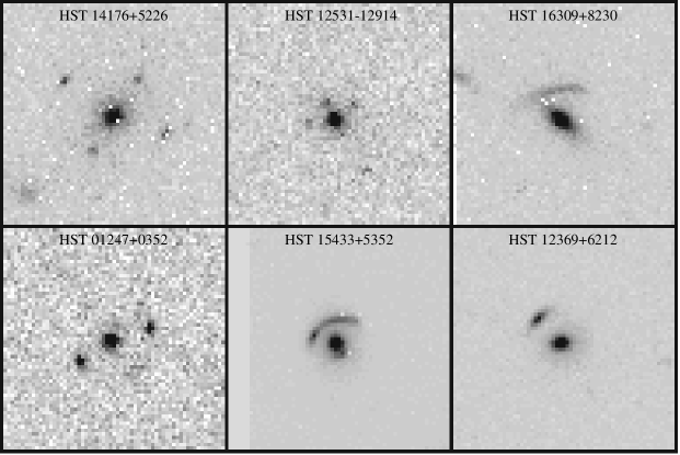
We selected the best six of the “Top Ten” MDS gravitational lens candidates (RGO99) and fitted them with these six models. These six lenses can be seen in Figure 1. Of the four that were not used, two were too faint, one was too close to the CCD edge where the PSF changes rapidly and one was found in a small group. These difficulties made these four lenses undesirable for comparison of the mass models. We used the same software procedure as used in RGO99 with the required modification to the potential.

Figure 1: WFPC2 F606W images of the six lenses used in this study. Each image is 6 $\farcs$4 x 6 $\farcs$4

We also attempted to model three previously reported lenses with HST images: PG1115+080 (Kristian et. al, 1993), MG0414+0534 (Falco, Lehar, Shapiro, 1997), and B1608+656 (Myers et. al, 1995). In all of these cases the lensed images are brighter than the lensing galaxy. The relative fluxes of the lensed components are well constrained by the high signal to noise ratio of these images but are poorly fit by simple lens models. This is a well known problem that can only be solved by using more complicated mass models which include substructure in the lens galaxy (Mao and Schneider, 1998). Since the fit and residuals were dominated by the poor fit to the lensed component fluxes they were also undesirable for comparison of mass models.

Given a set of model parameters, we generate 2-dimensional images for the elliptical and the source galaxies. The expected configuration of the lensed images is ray-traced. To improve the accuracy of this calculation, the image is evaluated using a pixel size smaller than the real one, such that the image fills a 64 pixel square array. The elliptical lens and the lensed source images are then convolved with the adopted HST WFPC2 point spread function from TinyTim (Krist, 2000). The convolved image is spatially integrated to the WFC pixel size of 0$\farcs$1 and is then compared with the observed galaxy image. The likelihood function is defined as the sum over all pixels of the logarithm of the probability of the observed value, assuming a Gaussian error distribution with respect to the model. This is proportional to a weighted $\chi^{2}$, and is then minimized using a quasi-newtonian method. The rms errors are estimated from the covariance matrix which is derived by inverting the Hessian at the maximum of the likelihood function. This method is sensitive not only to the location and magnitude of the lensed components but also to their shape and distortion. Once a best fit was found for each model we calculated the area within the caustic. The caustic is found by first calculating the image distortion which can be expressed by the Jacobian matrix:

$$A\left(\mathbf{x}\right)=\frac{\partial\mathbf{y}}{\partial\mathbf{x}}$$ (20)

Next the critical curves are found by solving $\det\mathbf{A}=0$. This solution is then inserted into the lens equation (eq. 1), giving the caustics. Most models have two caustics. However, some models (SIE and its variants as well as SSS for certain parameters) have only one. In these cases we calculate a cut which is a curve surrounding the region where multiple images exist, but which is not within the caustic (Kovner, 1987). The cut becomes a caustic if the singularity in the surface mass distribution is removed. The cut and caustic were computed analytically for SIE, SML, SIG and NIE using equations (slightly modified to include a shear term) found in KSB94. The cut and caustic for the SSS was also computed analytically, while the NFW’s caustics had to be determined numerically. The details of the cut and caustic equations can be found in the Appendix. The areas within the caustics and/or cut were then integrated numerically.

All six models used the standard parameters for modeling the light distribution of the lens galaxy: local sky, location (x,y), total magnitude, half-light radius, axis ratio and position angle. In addition, all models contained parameters describing the properties of the lensed source: x and y offset with respect to the lens galaxy, magnitude, half-light radius, axis ratio and orientation. Parameters describing the mass include the critical radius plus the following model dependent parameters: the axis ratio and orientation of the lens mass for the SIE and NIE models, a core radius for the NIE, a softness parameter for the SSS, and two parameters to describe the global shear (magnitude and direction) for the SSS, NFW, SML, and SIG. For all models the centroid of the gravitational potential of the lens was assumed to be the same as that of the light of the lensing galaxy. For reference the six models and a brief explanation of each are listed in Table 1.

Table 1: Explanation of mass models.

Model	Number of Parameters	Description
SIE	15	Singular Isothermal Ellipsoid.
SIG	16	Same as SIE with mass orientation the same as the light. Requires shear.
SML	15	Same as SIE with mass orientation & axis ratio the same as the light. Requires shear.
NIE	16	Isothermal Ellipsoid with a core radius (non-singular).
SSS	16	Singular Spherical model with a Softness parameter. Requires shear.
NFW	15	Spherical model from CDM simulations. Requires shear.

Unlike the fully automated Disk-plus-Bulge decomposition in the Medium Deep Survey pipeline (Ratnatunga, Griffiths, and Ostrander, 1999b), convergence of the lens model requires an initial guess in which the lensed images at least overlap the observed components. Since the number of discovered lenses is limited, we have so far worked out the initial guess by trial and error. We have also simplified the derivation of the initial guess by using a web based simulator. This form based cgi-driver, which includes all the model parameters, has been written in f77 using the same subroutines used in the lens analysis.

3 ANALYSIS

In most cases several models fit a given lens system equally well and rarely was any model strongly ruled out. This can be seen in Table 2 which shows the maximum likelihood for all lenses and passbands. For each lens, the likelihood values for each passband of a given model were summed. The best fit model is then just the model for which this sum is the smallest. Any other model with a summed likelihood which differs from the best by less than 5 times the number of passbands was considered to be statistically equivalent to the best model, although even models with much larger differences still gave reasonable fits to the lens systems.

Table 2: Maximum likelihood for each lens system and passband.

HST 01247+0352			HST 12369+6212
Model	F606W	F814W	Model	F606W	F814W	F450W
SIG	2536.7	2682.3	SSS	1924.2	3115.1	1613.9
SSS	2542.8	2682.2	SIG	1927.0	3115.9	1610.9
NFW	2560.8	2712.3	NFW	1927.1	3117.8	1610.3
SIE	2561.8	2702.5	NIE	1933.6	3105.6	1623.4
NIE	2562.4	2703.2	SIE	1934.2	3106.4	1623.5
SML	2564.8	2704.8	SML	1939.5	3121.9	1609.3
# of pixels	1902	1917	# of pixels	1281	1594	1168
HST 12531-2914			HST 15433+5352
Model	F606W	F814W	Model	F606W	F814W	F450W
SIG	1626.5	2057.5	SSS	3286.7	2913.9	1956.3
NFW	1627.8	2054.1	NFW	3321.2	2952.4	1950.8
SSS	1628.0	2055.5	SIG	3323.0	2944.8	1925.2
SML	1628.5	2054.8	SML	3327.3	2946.4	1934.5
NIE	1633.2	2053.0	NIE	3399.4	2975.4	1966.4
SIE	1636.7	2052.7	SIE	3399.6	2970.8	1971.1
# of pixels	1168	1416	# of pixels	1758	1780	1298
HST 14176+5226			HST 16309+8230
Model	F606W	F814W	Model	F606W	F814W	F450W
SIG	3403.8	4477.2	NFW	2039.5	2544.8	1864.8
NIE	3410.3	4466.5	SIE	2040.9	2546.1	1867.2
SIE	3410.4	4471.0	NIE	2043.1	2542.7	1864.4
SML	3415.3	4479.6	SSS	2045.2	2546.1	1868.9
SSS	3425.1	4487.4	SIG	2045.3	2547.7	1865.3
NFW	3447.2	4492.3	SML	2046.3	2548.4	1866.9
# of pixels	2453	3015	# of pixels	1528	1781	1438

The first lens (HST 14176+5226) was our best four-group image. Several models fit equally well including the SIE, NIE, and SIG. The SSS, NFW and SML models do not fit as well but are not strongly ruled out. The only other four group image was HST 12531-2914. All models gave indistinguishable results for this lens. The lens HST 01247+0352, which consists of a nearly spherical lens galaxy and two images of the source galaxy, was fit equally well with SSS and SIG while the remaining models were again not strongly ruled out. The other two-component lens image was HST 15433+5352 which was made up of an elliptical lens galaxy, a large arc, and a small source image opposite the arc. The SSS model was favored over the other models for this system: this is the only lens that favored just one model. The remaining two lenses modeled were both cases of a lens galaxy and a single arc. The first of these, HST 12369+6212, was from the Hubble Deep Field and was first reported by Hogg et. al (1996). It was modeled well by SSS, SIG, SIE, NIE, and NFW. The final lens, HST 16309+8230, showed no preference for any model. Thus many models give adequate fits to the same lenses, introducing a degeneracy in the parameters describing the mass of the lens systems. An example of the resulting caustic image for each system is shown in Figure 2 and Table 3 gives some of the parameters derived from modeling the systems in Figure 2. The full list of all parameters for all of the lens system can be found at the web site http://mds.phys.cmu.edu/lenses.

Figure 2: A sample of cut and caustic images in F606W. Short dashes show the interior caustic, long dashes are the outer caustic (or cut), and a thin/thick solid line represents the ellipse with the half light radius of the lens/source galaxy. The arrow shows the relative magnitude and direction of the shear where applicable.

Table 3: A sample of basic parameters in F606W.

Parameter	14176 $+$5226	01247 $+$0352	12369 $+$6212	16309 $+$8230	12531 $-$2914	15433 $+$5352
Model	SIE	SIG	NFW	NIE	SML	SSS
Lens Magnitude	21.84	23.95	23.96	21.61	23.89	21.86
Lens half-light radius ($arcsec$)	1.012	0.065	0.315	0.705	0.130	0.281
Lens position angle ($deg$)	$-$40.62	$-$38.67	$-$81.42	48.01	40.05	27.90
Lens axis ratio	0.67	1.00	0.71	0.35	0.64	0.71
Source x offset ($arcsec$)	$-$0.019	0.097	$-$0.577	$-$0.055	$-$0.029	$-$0.051
Source y offset ($arcsec$)	0.138	0.015	0.560	0.463	0.056	0.155
Critical Radius ($arcsec$)	1.496	1.085	0.440	0.414	0.595	0.577
Mass Axis Ratio	0.37	0.37	1.00:	0.59	0.64:	1.00:
Angle of Mass wrt Light ($deg$)	12.20	0.00:	0.00:	8.54	0.00:	0.00:
Source half-light radius ($arcsec$)	0.038	0.010	0.060	0.467	0.031	0.113
Source position angle ($deg$)	0.00:	0.00:	0.00:	$-$81.93	0.00:	$-$74.60
Source axis ratio	1.00:	1.00:	1.00:	0.15	1.00:	0.57
Softness parameter	1.00:	1.00:	NA	1.00:	1.00:	0.92
Core radius	0.000:	0.000:	0.000:	0.005	0.000:	0.000:
Shear magnitude	0.000:	0.300	0.295	0.000:	0.128	0.150
Shear direction ($deg$)	0.00:	$-$88.87	$-$51.34	0.00:	$-$33.40	3.04

The fact that four of the six models use a shear term allows us to investigate external shear for the lenses. Most of the lens systems required small values of shear roughly consistent with cosmic shear due to large scale structure (Casertano, Ratnatunga, and Griffiths, 1999). The only exceptions to this are HST 12369+6212 and HST 12531-2914 both of which require shears that are large compared to external shears expected from large-scale structure. In the case of 12531-2914 we find that a shear of $\approx 0.14$ is required to fit the observed configuration. This value is slightly less than the value of $\approx 0.20$ found by Witt and Mao (1997). This shear could be due to a nearby galaxy or by dropping the requirement that the mass of the lens be aligned with the light. Since there does not appear to be a galaxy at the require angle of $\approx-26{{}^{\circ}}$ we agree with the findings of Witt and Mao (1997) who concluded that the shear was due to a misalignment of mass and light. In fact, the lens system was well fit by allowing the mass to be rotated by $\approx-15{{}^{\circ}}$. HST 12369+6212 was found to have a shear term of $\approx 0.25$ at a direction of $\approx-54{{}^{\circ}}$. Two nearby objects (12:36:57.10+62:12:26.7 and 12:36:56.31+62:12:10.2) can be found in this direction which could explain this large shear. Although this lens was also well fit by allowing the position angle of the mass to vary the fitted angle was very large ($\approx-68{{}^{\circ}}$) making it a less attractive model.

We next compare in Figure 3 the fractional change in the critical radius as a function of the models fitted to each of the six gravitational lens systems. Since the critical radius is determined by the redshifts of the lens and source and the velocity dispersion of the lens we expect that it should not vary significantly between models. We find that the critical radius change is 4.3% rms. We note that the SSS and NFW model fits have a slightly smaller critical radius than SIE. This result confirms the theoretical expectation that if we were able to measure the velocity dispersion with an accuracy of a few km/s, then the cosmological constant could be directly estimated (Im, Griffiths and Ratnatunga, 1997).

Figure 3: Critical radius for each lens system and model. Square: F814W, triangle: F606W, and circle: F450W. Filled symbols represent the best fit models

The surface mass density distribution and the resulting potential gradient change lead to a small caustic centered on each lensing galaxy. For different potential models fitted to the same observed lens configuration, we see that the fractional change in the area within the caustic is much larger than that expected from the small change in critical radius. We note that the area within the interior caustic changes by 25% rms between models of the same lens configuration (Figure 4). The SSS and NFW models have a slightly smaller area within the caustic for strong gravitational lens cases. This result agrees well with Blandford and Kochanek (1987) which showed that shallower mass profiles (such as NFW and SSS with $\alpha$ less than 1.0) have smaller cross sections. This result indicates that the range of area within the caustic is a possible contributor to errors in the estimation of the number of detectable lenses expected from a survey.

Figure 4: Area within interior caustic for each lens system and model. Square: F814W, triangle: F606W, and circle: F450W. Filled symbols represent the best fit models

In a magnitude limited sample the discovery probability depends also on magnification. Figure 5 shows the variation in magnification for the various models. Since each model fits the observed magnitude, a lens model which has higher magnification implies a fainter source galaxy. Since there are more galaxies at fainter magnitudes, the discovery probability increases. However, we note (again in agreement with Blandford and Kochanek (1987)) that the models with larger magnification tend to have smaller caustics. Thus, these two effects oppose each other since a smaller caustic decreases the discovery probability.

Figure 5: Magnitude for each lens system and model. Square: F814W, triangle: F606W, and circle: F450W. Filled symbols represent the best fit models

Figure 6 graphically shows an example of how parameters can vary from model to model for a given lens system, in this case HST 14176+5226 which is the only spectroscopically confirmed lens. In particular, the size of the interior caustic changes significantly between models. Table 4 gives the values of many of the parameters in each model for this lens system.

Figure 6: Caustic and Cut images for HST 14176+5226 in F606W. Short dashes show the interior caustic, long dashes are the outer caustic (or cut), and a thin/thick solid line represents the ellipse with the half light radius of the lens/source galaxy. The arrow shows the relative magnitude and direction of the shear where applicable.

Table 4: A sample of key parameters for HST 14176+5226 F606W.

Parameter	SIE	SIG	SML	NIE	SSS	NFW
Mass Axis Ratio	0.37	0.38	0.64	0.39	1.00:	1.00:
Angle of Mass wrt Light ($deg$)	12.20	0.00:	0.00:	12.32	0.00	0.00
Shear Magnitude	0.00:	0.05	0.10	0.00:	0.31	0.15
Shear Direction ($deg$)	0.00:	49.16	18.39	0.00:	12.89	14.04
Critical Radius ($arcsec$)	1.496	1.498	1.401	1.522	1.359	1.374
Source Magnitude ($mag$)	26.16	26.14	26.41	26.20	25.52	26.96
Magnification ($mag$)	2.29	2.36	2.60	2.31	1.78	3.17
Caustic Area ($arcsec^{2}$)	1.11	1.05	0.58	1.06	0.92	0.25

4 CONCLUSIONS

We have investigated different potentials and found that it is difficult in most cases to distinguish between them.

We observe that the critical radius is fairly constant for a particular lens system, independent of the model used. The critical radius is determined by the distances to the lens and source galaxy, which are measurable observables, and the integrated mass. Since we see only small variations across the various models, this implies that the integrated mass is not significantly different from model to model.

However, even models that lead to very similar lensed image configurations have very different caustics. Since the area within the caustic and the magnification determine the creation and discovery of strong lenses, these differences, along with the faint galaxy count distribution, change the expected number of detected lenses. Any attempt to determine the cosmological constant from such numbers must take these factors into consideration.

We note that samples of radio gravitational lens candidates are discovered by detecting a compact multiple component image structure with identical spectral characteristics. This sample, although well defined, discovers mainly lenses of QSO sources, and otherwise depends on the radio characteristics of faint galaxies. On the other hand optical gravitational lens candidates detected without spectral observations need to be based on the likelihood of the configuration compared with random clustering of galaxies. A single faint blue galaxy in proximity to a red elliptical galaxy is not a reliable lens candidate, since such configuration very frequently happens by chance. However, four galaxies in a cross pattern around an elliptical galaxy is a reliable lens candidate since the chance of this occurring at random is very small. In the process of this study we examined several radio lenses with HST data and found that in most cases, we would not have identified the lens based only on the WFPC2 image. Likewise, many of the lenses in our sample, in particular HST 14176+5226 and HST 12531-2914, were not detected by observations made on the VLA. These two methods (radio and optical) seem to find different lens candidate samples which complement each other, allowing a better understanding of selection effects.

The discovery probability for optically discovered lenses is affected by the symmetry of the configuration, the contrast of source color against that of the lens galaxy, and the critical radius. If a distant galaxy happens by chance to fall within the caustic of a foreground galaxy we observe four images of the source known as a ‘strong’ gravitational lens. If these images are about one magnitude brighter than the object detection threshold, with a critical radius larger than about 0.4 arcsecond, then we are confident that we would discover the lens with high reliability. As the intrinsic location of the source passes outside the caustic, three of the multiple images merge into one and the fourth image on the opposite side becomes much fainter, and may not be visible. Between the caustic and either the outer caustic or cut two images are formed. This is also the special case of perfect spherical symmetry and no external shear when the central caustic vanishes. As the source location nears the second caustic (or the cut) one image will become fainter making only one image (highly distorted) visible. We do not expect to discover these lens systems unless the source galaxy is extended with a half light radius larger than about 0.1 arc seconds. We refer to these cases as ‘mild’ lensing. For instance if the source galaxy is intrinsically extended and almost spherical, then it would be seen to form a prominent arc oriented with the curvature centered on the lensing galaxy. This makes a probable lens. If however the original was extended but with a large ellipticity, then it would look like a nearby galaxy with random orientation.

The variety of possible lens configurations is numerous. We can investigate the discovery probability using the fully interactive simulator which we have made available publicly on the web at http://mds.phys.cmu.edu/lenses. This interactive tool can not only provide an initial guess to match a new lens configuration but can also allow us to explore the multi-dimensional parameter space to investigate the probability of discovery. We urge the reader to visit this web site and try it. All models, model parameters, and cosmological parameters can be selected. The source location relative to the caustic can be input via a line diagram of the caustic and cut. A color image is created of the lensed source and lensing galaxy.

This paper is based on observations with the NASA/ESA Hubble Space Telescope, obtained at the Space Telescope Science Institute, which is operated by the Association of Universities for Research in Astronomy, Inc., under NASA contract NAS5-26555. The HST Archival research was funded by STScI grant GO8384.

Appendix A APPENDIX

The general method for finding the caustic for a lens was discussed above. Here we give more specific details on finding the caustic for the SSS model and a small correction that was need for the NIE. The caustic equations for SIE can be found in KSB94.

For NIE $\det\mathbf{A}=0$ is equivalent to

$$8c_{3}\kappa^{3}+4c_{2}\kappa{2}+2c_{1}\kappa+c_{0}=0$$ (A1)

as in KSB94 with the following correction to the coefficients:

$$c_{3}=\left(x_{c}f^{3/2}-x_{c}^{2}-x_{c}^{2}f^{2}\right)\Delta^{2}+x_{c}^{2}f^{2}$$ (A2)

$$c_{2}=\left(-2x_{c}f^{3/2}+x_{c}^{2}+x_{c}^{2}f^{2}\right)\Delta^{2}-x_{c}^{2}f^{2}$$ (A3)

$$c_{1}=2x_{c}f^{3/2}\Delta^{2}-f^{3}$$ (A4)

$$c_{0}=f^{3}.$$ (A5)

The resulting critical curve is then used in the lens equation to give the caustic. For SSS solving $\det\mathbf{A}=0$ gives the critical curve

$$x=\kappa_{0}\left[\frac{P-\sqrt{P^{2}-4\left(\beta-1\right)\left(1-\gamma^{2}\right)}}{2\left(\beta-1\right)}\right]^{\frac{1}{\beta-2}}$$ (A6)

where

$$P=\beta-\gamma\left(\beta-2\right)\cos\left(2\varphi-2\theta_{\gamma}\right)$$ (A7)

which gives the caustic

$$y_{1}=x\cos\varphi-\kappa_{0}^{\left(2-\beta\right)}x^{\beta-1}+x\gamma\left[\cos\phi\cos\left(2\theta_{\gamma}\right)+\sin\phi\sin\left(2\theta_{\gamma}\right)\right]$$ (A8)

$$y_{2}=x\sin\varphi-\kappa_{0}^{\left(2-\beta\right)}x^{\beta-1}+x\gamma\left[\cos\phi\sin\left(2\theta_{\gamma}\right)-\sin\phi\cos\left(2\theta_{\gamma}\right)\right].$$ (A9)

The caustic for the NFW model was found by numerically solving the Determinate of $\mathbf{A}$ and putting the resulting critical curve back into the lens equation.

References

- Blandford and Kochanek (1987) Blandford, R. D. & Kochanek, C. S. 1987, ApJ, 321, 658
- Casertano, Ratnatunga, and Griffiths (1999) Casertano, S., Ratnatunga, K. U., & Griffiths, R. E., in Proc Gravitational Lensing: Recent Progress and Future Goals eds: T. G. Brainerd and C. S. Kochanek. (PASP)
- Cohen et. al (2000) Cohn, J. D., Kochanek, C. S., McLeod, B. A., & Keeton, C. R. 2000, ApJ in press, astro-ph/0008390
- Crampton et. al (1996) Crampton, D., Le Févre, O., Hammer, F., & Lilly, S. J. 1996, A&A, 307, L53
- Falco, Lehar, Shapiro (1997) Falco, E. E., Lehar, J., & Shapiro, I. I. 1997, AJ, 113, 540
- Im, Griffiths and Ratnatunga (1997) Im M., Griffiths, R. E., & Ratnatunga, K. U. 1997, ApJ, 475, 457
- Hogg et. al (1996) Hogg, D. W., Blandford, R., Kundić, T., Fassnacht, C. D., & Malhotra, S. 1996 ApJ, 467, L73
- Kochanek (1995) Kochanek, C. S. 1995, ApJ, 445, 559
- Kormann, Schneider and Bartelmann (1994) Kormann, R., Schneider, P., & Bartelmann, M. 1994 A&A, 284 285 (KSB94)
- Kovner (1987) Kovner, I. 1987, ApJ, 312, 22
- Krist (2000) Krist, J. 2000, The TINYTIM User’s Manual (Baltimore: STScI)
- Kristian et. al (1993) Kristian, J. et. al 1993, AJ, 106, 1330
- Mao and Schneider (1998) Mao, S., Schneider, P. 1998, MNRAS, 295, 587
- Mellier (1999) Mellier, Y. 1999, ARAA, 37, 127
- Myers et. al (1995) Myers, S. T. et. al 1995, ApJ, 447, L5
- Navaro, Frenk, and White (1995) Navaro, J., Frenk, C. S., & White S. D. M. 1995 MNRAS, 275, 720
- Ratnatunga et al. (1995) Ratnatunga, K. U., Ostrander, E. J., Griffiths, R. E. & Im, M. 1995, ApJ, 453, L5
- Ratnatunga, Griffiths, and Ostrander (1999a) Ratnatunga, K. U., Griffiths, R. E. & Ostrander, E. J. 1999a, AJ, 117, 2010 (RG099)
- Ratnatunga, Griffiths, and Ostrander (1999b) Ratnatunga, K. U., Griffiths, R. E. & Ostrander, E. J. 1999b, AJ, 118, 86
- Witt, Mao, and Schechter (1995) Witt, H. J., Mao, S., & Schechter, P. L. 1995, ApJ, 443, 18
- Witt and Mao (1997) Witt, H. J., Mao, S. 1997, MNRAS, 291, 211